www.atmos-meas-tech.net/7/2839/2014/ doi:10.5194/amt-7-2839-2014
© Author(s) 2014. CC Attribution 3.0 License.
Remote sensing of cloud top pressure/height from SEVIRI:
analysis of ten current retrieval algorithms
U. Hamann1,2, A. Walther3, B. Baum3, R. Bennartz3,4, L. Bugliaro5, M. Derrien6, P. N. Francis7, A. Heidinger8, S. Joro9, A. Kniffka10, H. Le Gléau6, M. Lockhoff10, H.-J. Lutz9, J. F. Meirink1, P. Minnis11, R. Palikonda12, R. Roebeling9, A. Thoss14, S. Platnick13, P. Watts9, and G. Wind13
1Royal Netherlands Meteorological Institute (KNMI), De Bilt, the Netherlands 2MeteoSwiss, Locarno, Switzerland
3University of Wisconsin, Madison, WI, USA 4Vanderbilt University, Nashville, TN, USA
5Deutsches Zentrum für Luft- und Raumfahrt, Institut für Physik der Atmosphäre, Oberpfaffenhofen, Germany 6Météo-France, Lannion, France
7Met Office, Exeter, UK
8Center for Satellite Applications and Research, NESDIS, NOAA, Madison, WI, USA 9EUMETSAT, Darmstadt, Germany
10Deutscher Wetterdienst (DWD), Offenbach, Germany 11NASA Langley Research Center, Hampton, VA, USA 12Science Systems and Applications, Inc., Hampton, VA, USA 13NASA Goddard Space Flight Center, Greenbelt, MD, USA
14Swedish Meteorological and Hydrological Institute (SMHI), Norrköping, Sweden Correspondence to: U. Hamann (ulrich.hamann@meteoswiss.ch)
Received: 14 November 2013 – Published in Atmos. Meas. Tech. Discuss.: 20 January 2014 Revised: 11 July 2014 – Accepted: 14 July 2014 – Published: 9 September 2014
Abstract. The role of clouds remains the largest uncertainty in climate projections. They influence solar and thermal ra-diative transfer and the earth’s water cycle. Therefore, there is an urgent need for accurate cloud observations to vali-date climate models and to monitor climate change. Passive satellite imagers measuring radiation at visible to thermal in-frared (IR) wavelengths provide a wealth of information on cloud properties. Among others, the cloud top height (CTH) – a crucial parameter to estimate the thermal cloud radiative forcing – can be retrieved. In this paper we investigate the skill of ten current retrieval algorithms to estimate the CTH using observations from the Spinning Enhanced Visible and InfraRed Imager (SEVIRI) onboard Meteosat Second Gener-ation (MSG). In the first part we compare ten SEVIRI cloud top pressure (CTP) data sets with each other. The SEVIRI al-gorithms catch the latitudinal variation of the CTP in a sim-ilar way. The agreement is better in the extratropics than in the tropics. In the tropics multi-layer clouds and thin cirrus
layers complicate the CTP retrieval, whereas a good agree-ment among the algorithms is found for trade wind cumu-lus, marine stratocumulus and the optically thick cores of the deep convective system.
than to CALIOP measurements. The biases between SEVIRI and CPR retrievals range from−0.8 km to 0.6 km. The cor-relation coefficients of CPR and SEVIRI observations vary between 0.82 and 0.89. To discuss the origin of the CTH de-viation, we investigate three cloud categories: optically thin and thick single layer as well as multi-layer clouds. For op-tically thick clouds the correlation coefficients between the SEVIRI and the reference data sets are usually above 0.95. For optically thin single layer clouds the correlation coeffi-cients are still above 0.92. For this cloud category the SE-VIRI algorithms yield CTHs that are lower than CALIOP and similar to CPR observations. Most challenging are the multi-layer clouds, where the correlation coefficients are for most algorithms between 0.6 and 0.8. Finally, we evaluate the performance of the SEVIRI retrievals for boundary layer clouds. While the CTH retrieval for this cloud type is rel-atively accurate, there are still considerable differences be-tween the algorithms. These are related to the uncertainties and limited vertical resolution of the assumed temperature profiles in combination with the presence of temperature in-versions, which lead to ambiguities in the CTH retrieval. Al-ternative approaches for the CTH retrieval of low clouds are discussed.
1 Introduction
About 70 % of the earth’s surface is covered with clouds. They play an essential role in weather and climate inter-acting strongly with solar and terrestrial radiation (Cess et al., 1989). In the solar wavelength region, clouds cool the earth by reflecting sunlight back to space. At the same time clouds tend to warm the earth by absorbing and re-emitting thermal radiation emitted by the surface and lower atmo-sphere (Wielicki et al., 1995). While solar radiative transfer is mainly influenced by the cloud cover and the optical depth of the clouds, the thermal effect is also determined by their cloud top temperature. Thus, optically thick, low level clouds usually have a negative net radiative forcing as their thermal effect is small and reflection of solar radiance dominates. In contrast, the net radiative effect of high level clouds is of-ten positive (in particular during night and for optically thin cirrus over warm surfaces during day) because the thermal contrast between them and the surface is large (Liou, 1986; Boucher, 1999; Meyer et al., 2002; Schumann et al., 2012).
Hence, detailed monitoring of cloud properties – such as cloud fraction, cloud top temperature, cloud particle size and cloud water path – is needed to understand the role of clouds in the weather and climate system. Cloud remote sensing from space is an important and effective tool to monitor cli-mate change and to evaluate weather and clicli-mate models. Satellites are able to observe cloud properties globally, and, in particular, passive imagers provide observations of large areas with a high temporal resolution enabling investigations of the evolutions and life times of cloud systems.
The International Satellite Cloud Climatology Project (IS-CCP) has monitored cloud properties including cloud top temperature and pressure as well as cloud water path and cloud optical depth since 1983 from geostationary satel-lites and the Advanced Very High Resolution Radiometer (AVHRR) on the polar orbiting NOAA and MetOp satellites (Rossow and Schiffer, 1999). But little information about cloud phase, particle size and night time cloud heights is provided as only two satellite channels are used for tempo-ral consistency. Many other techniques have been developed since the start of ISCCP to derive those additional parameters utilizing multiple channels now available on most modern geostationary and sun-synchronous satellite imagers. In par-ticular, the use of more channels in the visible to long-wave infrared (IR) wavelength region (400 nm–15 µm) is very ben-eficial.
Despite the progress in this area, the interpretation of the measured radiance remains challenging for the following reasons: first, observations do not fully constrain the retrieval problem. Most information originates from the cloud top, but clouds are vertically extended and have a complex struc-ture. Second, satellite pixels typically cover an area of a few km2. The clouds within this area are inhomogeneous. Radia-tion from neighboring areas as well as the three-dimensional structure of clouds influence the observed radiance, which is normally neglected in cloud remote-sensing algorithms (e.g., Zinner and Mayer, 2006). Hence, the common assumption of a plane parallel single cloud layer can only approximate re-ality. Third, the thermal emission of the cloud comes from within the uppermost cloud layer. Therefore, the retrieved cloud top height (CTH) is a radiatively effective one and not the physical cloud boundary. Fourth, in case of temperature inversions, the conversion from observed brightness temper-ature to CTH can be ambiguous and may lead to large dis-placements. Furthermore, during the day retrievals are chal-lenging for certain observation geometries such as the sun glint angular envelope and high solar zenith angles. Finally, a number of facts are only partially known: the shapes of ice crystals that determine their scattering and absorption prop-erties, the state of the atmosphere, the albedo and emissivity of the surface, calibration and degradation of the satellite sen-sor and uncertainties in the spectral response function. This limited knowledge exacerbates cloud remote sensing in prac-tice even more, especially for optically thin clouds. The ra-diative effect of these uncertainties can be significant com-pared to the cloud effect itself and, therefore, retrieved cloud properties may also be uncertain.
imagers, IR sounders and active instruments. Stubenrauch et al. (2013) stated that CTH measurements are comparable considering the different sensor sensitivities. In particular, they pointed out that passive imagers measure a radiatively effective CTH. Furthermore, the GEWEX cloud assessment investigated the regional and vertical distributions as well as diurnal and seasonal cycles.
As averaged cloud properties are used in the GEWEX cloud assessment, differences of the Level 2 to Level 3 ag-gregation procedure as well as differences among the re-trieval methods themselves are identified as cause for the observed deviations. Therefore, an additional in-depth anal-ysis of Level 2 cloud products reveal even more insight into the characteristics of retrieval algorithms. This is why the Cloud Retrieval Evaluation Workshop (CREW) project was founded (Roebeling et al., 2012). Exchanges during the CREWs in 2006, 2009 and 2011 triggered the creation of a cloud retrieval database. A large number of research groups provided their retrieval results to this database, thus enabling a systematic evaluation similar to the GEWEX cloud as-sessment, but for Level 2 products. This is the first effort of its kind since the pre-ISCCP algorithm inter-comparisons (Rossow et al., 1985).
The current paper presents the inter-comparison and vali-dation results of ten CTH retrieval algorithms using observa-tions of the Spinning Enhanced Visible and InfraRed Imager (SEVIRI) onboard the geostationary Meteosat Second Gen-eration (MSG) platform using the CREW database. The pa-per is structured as follows: in Sect. 2 we give a description of the satellite sensors used, review the fundamentals of cloud top height/pressure retrieval methods and give an overview of the Cloud Retrieval Evaluation Workshop database. In Sects. 3 and 4 we present the results of the SEVIRI retrieval inter-comparison and the comparison with Cloud–Aerosol LIdar with Orthogonal Polarization (CALIOP) and CPR. In Sect. 5 we discuss and summarize our findings.
2 Data sets and methods
Section 2.1 summarizes the characteristics of the satellite sensors used in this study. In Sect. 2.2 we introduce com-mon retrieval methods for clouds from passive sensors in general, followed by a description of the CREW cloud re-trieval database in Sect. 2.3.
2.1 Instrumentation
In this paper we inter-compare retrievals using observations from the SEVIRI instrument (Schmetz et al., 2002) on the geostationary Meteosat-9 satellite located at the orbital posi-tion 0◦E and 0◦N. Observations are possible up to a view-ing zenith angle of ca. 70◦ thus including mainly Africa, Europe, the Atlantic Ocean as well as small parts of South America and the Indian Ocean. SEVIRI has eleven spectral
bands with 3 km spatial resolution at the sub-satellite point: three solar channels at 0.6, 0.8 and 1.6 µm, one combined so-lar/thermal channel at 3.9 µm, two water vapor channels at 6.2 and 7.3 µm, one ozone channel at 9.6 µm, one CO2 chan-nel at 13.4 µm and three IR window chanchan-nels at 8.7, 10.8 and 12.0 µm. The seven thermal channels are calibrated on-board, while the solar channels are not and require vicari-ous calibration (Govaerts et al., 2001). Furthermore, SEVIRI has one high-resolution broadband visible (HRV) channel at 1 km spatial resolution. The SEVIRI sensor scans the obser-vation disk every 15 min. The scan starts in the south and takes 12 min to reach the northernmost point. The high tem-poral resolution enables the study of the evolution of cloud systems including the diurnal cycle.
In the second part of the paper, we compare the CTH retrievals from SEVIRI with measurements from active in-struments, namely the Cloud–Aerosol LIdar with Orthogo-nal Polarization (CALIOP) and the Cloud Profiling Radar (CPR). CALIOP is the main instrument on the CALIPSO satellite launched in April 2006 (Winker et al., 2003, 2007, 2010; Liu et al., 2005; Hostetler et al., 2006); it is a dual wavelength lidar (532 and 1064 nm). The primary products are profiles of total backscatter, from which further products like cloud and aerosol properties are derived (Vaughan et al., 2005). The instrument also measures the linear depolariza-tion of the backscattered return signal at 532 nm allowing for the discrimination of cloud phase and the identification of non-spherical aerosols. On the earth’s surface individual CALIOP beams have a width of about 70 m with a sampling distance of 333 m. The vertical resolution of the CALIOP products is 30 to 60 m. The lidar retrieval is based on the lidar equation (Hostetler et al., 2006):
Er(λ, r)=Et dr A0
r2 k(λ) β(r) T
2(r), (1)
whereErandEt are the received and transmitted energy,r is the range from the lidar, dr the range resolution, λ the wavelength of the transmitted pulse andβ(r)the atmospheric backscatter coefficient.A0/r2is the acceptance solid angle of the receiving optics withA0being the collecting area of the telescope. The instrument constant k(λ) considers the response of the receiver like the spectral transmission. The signal is attenuated according to the two-way transmission
over several lidar shots. In this way, sub-visible clouds with a very small optical depth down to 0.01 can be detected. Its high sensitivity and vertical resolution make CALIOP an ex-cellent system for the validation of CTH retrievals from pas-sive radiometers.
The CPR onboard CloudSat launched in April 2006 is a 94 GHz nadir-looking radar. It measures the backscattered signal as a function of distance from the radar (Stephens et al., 2002, 2008; Tanelli et al., 2008). As clouds are weak scatterers in the microwave region, the CPR is designed for maximal sensitivity. Its dynamic range is 70 dB and its cali-bration accuracy is 1.5 dB. The attenuation of the radar sig-nal is influenced by absorbing gases (primarily water vapor), water and ice clouds as well as precipitating particles. With a pulse length of 3.3 µs, CPR provides cloud and precipita-tion informaprecipita-tion with 500 m vertical resoluprecipita-tion between the surface and 30 km. The radar measurements along track are averaged over 0.32 s time intervals, producing a horizontal resolution of 1.4 km (cross-track) by 1.7 km (along-track). The radar signal is interpreted with the radar equation
Er(λ, r)=Et 1
(4π )3r2L a
λ2σ GrG2 1, (2) whereEris the output energy of the receiver,Etthe transmit-ted energy,λthe wavelength,σthe range resolved radar cross section per unit volume,Grthe receiver gain,Gthe antenna gain, r the range to the atmospheric target, the integral of the normalized two-way antenna pattern, 1 the integral of the received waveform shape andLa the two-way atmo-spheric loss. As meteorological radars work in the Rayleigh regime, the extinction efficiency is less compared to the Mie regime; hence, radar can penetrate further into the cloud. The radar cross section can be written as
σ =π 5
λ4|K|
2X
i
D6i, (3)
whereDi is the diameter of the scattering particles.|K|2is
defined as |K|2=
εd−1
εd+2 2 , (4)
whereεdis the dielectric constant. For CPR|K|2=0.683 for
water and|K|2=0.176 for ice (Ray, 1972). Consequently, the reflectivity of water particles is around 0.683/0.176= 3.88 or 5.89 dBz higher for water particles than for ice par-ticles of the same size and shape. As the volumetric radar cross sectionηis proportional toDi6, the radar is much more sensitive to larger particles than to smaller ones.
2.2 Cloud top height retrieval methods
With observations of the radiance and a priori information of the atmospheric state, in particular the temperature pro-file and concentration of absorbing gases, the radiatively ef-fective CTH can be retrieved representing the top height of
a plane parallel, homogeneous cloud that cause the same ra-dianceIνat the top of the atmosphere as observed. In general,
the measured radianceIν at wave numberνdepends on the
cloud top pressurepcas follows (Liou, 2002):
Iν=(1−ηεν)(Is+Ib) tν(pc,0)+Ic+Ia, (5) where the contribution from the surface is described by
Is=Bν(Ts)tν(ps, pc), (6) the contribution of the atmosphere below the cloud by
Ib= pc Z
ps
Bν(T (p))
∂tν(p, pc)
∂p dp, (7)
the contribution of the cloud itself by
Ic=ηενBν(Tc)tν(pc,0), (8) and the contribution of the atmosphere above the cloud by
Ia= 0 Z
pc
Bν(T (p))
∂tν(p,0)
∂p dp. (9)
In these equationsηis the cloud fraction,εν the spectral
emissivity of the cloud,Bν the Planck radiation,tν(p1, p2) the transmissivity between pressuresp1andp2andpc,ps,
TcandTsare pressure and temperature of the cloud and the surface, respectively.
2.2.1 Radiance fitting
One basic method to derive the cloud top pressure (CTP) as-sumes a fully covered field of viewη=1 and optically thick cloudsεν=1. The term 1−ηεν on the right hand side in
Eq. (5) vanishes, being tantamount to no contribution from the surface and the atmosphere below the cloud. Assuming an atmospheric temperature and humidity profile, the radi-ance can be calculated using a radiative transfer model. The CTP is found by minimizing the difference between the sim-ulated and observed radiance. With this method and under the above-mentioned assumptions, the CTP can be derived by using only a single channel. It is favorable to use a wave-length with a large atmospheric transmissivity to minimize the influence of the atmosphere above the cloud on the re-trieval. For SEVIRI, the 10.8 µm channel is commonly cho-sen. It is possible to extend this retrieval method taking cloud cover η and/or the spectral cloud emissivity εν explicitly
into account (Chahine, 1974; Wielicki and Coakley Jr, 1981; Roebeling et al., 2006; Roebeling, 2008). The cloud coverη
can be estimated using the high-resolution channel of SE-VIRI. Furthermore, the spectral emissivity εν can be
cloud optical depths at visible and IR window-channel wave-lengths. Rossow and Schiffer (1999) solve first for the visi-ble optical depthτvis using the reflected radiance. Then, the emissivityεν is computed as
εν=1−exp(−0.5τvis/µ), (10) where µis cosine of the viewing zenith angle. Taking the semi-transparency and coverage of the cloud layer into ac-count, the retrieval results of the radiance fitting method can be significantly improved.
In the following we call this retrieval method radiance fit-ting. It is known that this method tends to overestimate CTP for partial cloud cover and semi-transparent clouds, if these effects are not taken into account (e.g., Holz et al., 2006). 2.2.2 Optimal estimation
A generalization of the radiance fitting is the optimal esti-mation (OE) method. It uses several channels and any avail-able prior information with suitavail-able weighting according to errors. Essential diagnostic outputs of the OE method are a measure of the model fit to the observation, that is, the cost function J, and formal error estimates of the retrieved pa-rameters. The cost functionJis defined as follows (Rodgers, 2000):
J (x)=(y(x)−ym)TS−y1(y(x)−ym)
+(x−xa)TSa−1(x−xa), (11) where ym are the measurements and y(x) are the radi-ances simulated by assuming the state x. xa is an esti-mate of the state prior to the retrieval and S−y1 and S−a1 are the inverted error covariance matrices of the measure-ments and the prior state, respectively. The state vector x is varied to minimize the cost function J yielding the op-timal state given the observation ym, the prior knowledge, and their respective uncertainties. In the context of this pa-per, the state parameter x contains the physical properties of the cloud. Using a window channel alone leads to very large solution spaces for CTP retrievals for cirrus, while the inclusion of a single absorbing channel greatly decreases the solution space (Heidinger et al., 2010). This is an ap-proach commonly adopted for use with SEVIRI as well as other polar-orbiting imagers. Iterative techniques can also be used to simultaneously fit more than one parameter to the same number of channels. Among others, OE has been applied to AVHRR (Walther and Heidinger, 2012), Along-Track Scanning Radiometer (ATSR) (Poulsen et al., 2011), SEVIRI (Watts et al., 2011), a combined Medium Resolu-tion Imaging Spectrometer (MERIS) and Advanced Along-Track Scanning Radiometer (AATSR) data set (Lindstrot et al., 2010) and Michelson Interferometer for Passive At-mospheric Sounding (MIPAS) (Hurley et al., 2011).
2.2.3 Radiance ratioing
Another approach to retrieve CTP is the radiance ratioing method (also sometimes named split window or CO2slicing) (Chahine, 1974; Cavia and Tomassini, 1978; Smith and Platt, 1978; Menzel et al., 1983, 2008; Wylie and Menzel, 1989; Zhang and Menzel, 2002). Subtracting the clear sky radiance
Iνclrfrom the all sky observationIνin Eq. (5) and integration
by parts leads to
Iν−Iνclr=ηεν pc Z
ps
tν(p,0)
∂Bν(T (p))
∂p dp, (12)
see, e.g., Liou (2002). The clear sky radiance can be simu-lated with a radiative transfer model or estimated by locat-ing clear sky measurements in the vicinity of the observa-tion (Smith and Frey, 1990). For radiance ratioing, Eq. (12) for a wave numberν1 is divided by the same equation for a second wave numberν2; hence, the formulation becomes independent of the cloud fractionη. Channel combinations for radiance ratioing are preferably chosen in that way that the gaseous absorptions forν1andν2 are different, but the spectral cloud emissivitiesεν are similar. For hyperspectral
sounders, e.g., Atmospheric InfraRed Sounder (AIRS), com-monly used channel combinations are located around 15 µm using the absorption feature of CO2; hence, this technique is called CO2slicing. The retrieval uncertainty depends on the atmospheric temperature and trace gas profiles (Holz et al., 2006; Smith and Frey, 1990) and, if not taken explicitly into account, on the spectral change of the cloud emissivity. Ac-curate calculation of the latter is shown to improves the CTP retrieval accuracy (Zhang and Menzel, 2002). For the SE-VIRI instrument, the 10.8 µm channel is commonly used in combination with the 12.0 or 13.4 µm channel. The wave-lengths of the satellite channels are further apart from each other for SEVIRI than for IR sounders, so that a calculation of the cloud emissivities is necessary. Parameterizations of cloud long-wave radiative properties are used for this pur-pose (e.g., Hu and Stamnes, 1993; Baum et al., 2005a, b, 2007).
2.3 The CREW database
In the framework of the Cloud Retrieval Evaluation Work-shop (CREW), a common cloud retrieval database was built to investigate strengths and weaknesses of currently avail-able cloud property retrieval algorithms using passive im-ager observations. The cloud properties stored in the CREW database are listed in Table 1.
Table 1. Cloud properties in the CREW database.
Acronym Cloud parameter
CMK Cloud mask CPH Cloud phase
CTT Cloud top temperature CTP Cloud top pressure CTH Cloud top height COD Cloud optical depth REF Effective radius LWP Liquid water path IWP Ice water path
Table 2. Days and core hours of the CREW database.
Date Core hours A-train orbit numbers
13 Jun 2008 12:00–15:30 11317, 11318, 11319 17 Jun 2008 22:15–24:00 11381, 11382 18 Jun 2008 00:00–01:45 11383 22 Jun 2008 10:30–12:15 11447, 11448 3 Jul 2008 10:00–12:00 11607, 11608, 11609
(POLDER) and the AIRS retrievals are included in the database. The database is complemented with cloud mea-surements that serve as a reference, including the Advanced Microwave Scanning Radiometer for EOS (AMSR-E) ob-servations and the active instruments CPR on CloudSat and CALIOP on CALIPSO.
The CREW database contains five days of data, see Ta-ble 2. During these days the NOAA-18 satellite was aligned with the A-train orbit for several hours. In this paper we fo-cus on 13 June 2008, as the data set is most complete for this day.
In total, twelve institutions from Europe and USA partic-ipate in the CREW inter-comparison and validation of their SEVIRI data sets. This paper investigates the ten data sets providing cloud top height or cloud top pressure retrievals. The acronyms and contact persons of the participating insti-tutions are listed in Table 3.
As a first step the raw signal measured by SEVIRI is con-verted into a radiance. Most of the algorithms use the L1 radiance product as provided by EUMETSAT. Only a few algorithms use an alternative calibration. The CMS algo-rithm uses the calibration described by Meirink et al. (2013). The LAR algorithm uses an additional calibration for the 0.65 µm channel against the Aqua MODIS channel and a cal-ibration for the 3.9 µm channel against GOES measurements (Minnis et al., 2002a, b). The UKM algorithm uses an ad hoc calibration for the 13.4 µm channel. Recent research in the framework of the Global Space-based Inter-Calibration Sys-tem (GSICS) demonstrated that the 13.4 µm is probably bi-ased by contamination with ice (Hewison and Müller, 2013). GSICS provides time-dependent calibration coefficients for
Table 3. Participating institutions.
Acronym Institute Contact person
AWG NOAA – CIMSS A. Heidinger, A. Walther CMS CM SAF A. Kniffka, M. Lockhoff
DLR DLR L. Bugliaro
EUM EUMETSAT H.-J. Lutz
GSF NASA Goddard S. Platnick, G. Wind LAR NASA Langley P. Minnis, R. Palikonda MFR Météo-France H. Le Gléau, M. Derrien MPF EUMETSAT S. Joro
OCA EUMETSAT P. Watts UKM UK Met Office P. Francis
the SEVIRI IR channels according to an inter-calibration against Metop-A IASI. The GSICS methodology of post-calibration is very advanced. At the moment none of the SE-VIRI algorithms uses the GSICS calibration coefficients. To estimate the benefit of the GSICS calibration on the CTH retrieval, a small case study is performed with the CMS al-gorithm for the 13 June 2008, 12:00 UTC. The effects on the retrieval results are small in comparison to the fundamental observation differences of the different sensors and the devi-ations among the SEVIRI algorithms discussed later in this paper. Nevertheless, the GISCS calibration changes the CTH retrieval results for some individual cases by up to 12 km. As GSICS provides the most sophisticated calibration, tak-ing advantage of it will certainly be beneficial for every al-gorithm.
After the calibration of the radiance, the CTP/CTH is de-rived. All variants of CTP retrieval methods discussed in Sect. 2.2 are applied in one or more algorithms. An overview of the retrieval methods and satellite channels used by the SEVIRI retrieval algorithms is given in Table 4. Many algo-rithms apply a combination of several methods. For optically thick and low clouds, many groups use radiance fitting with the IR window channel at 10.8 µm. For semi-transparent or broken clouds it is necessary to employ the radiance ratio-ing method. But the algorithms use different criteria for the identification of cloud regimes for which radiance ratioing is applied.
Table 4. SEVIRI cloud top height retrieval methods.
Acro. Method Channels (µm) Aux. data Citations
AWG optimal estimation 10.8, 12.0, 13.4 NCEP Menzel et al. (2008); Heidinger and Pavolonis (2009); Heidinger et al. (2010); Baum et al. (2012)
CMS (1) radiance fitting 10.8 ERA interim Derrien and Le Gléau (2005, 2010, 2013); (2) intersection method 6.2, 7.3, 10.8, 13.4 Schmetz et al. (1993); Appendix C; (3) radiance ratioing 6.2, 7.3, 10.8, 13.4 Menzel et al. (1983)
DLR (1) radiance fitting 10.8 ECMWF Meerkötter and Bugliaro (2009); Bugliaro et al. (2011); (2) radiance ratioing 10.8, 13.4 Ewald et al. (2013)
EUM (1) radiance fitting 10.8 ECMWF Lutz et al. (2011) (2) radiance ratioing 6.2, 7.3, 10.8, 12.0, 13.4
GSF (1) optimal estimation 3.9, 8.7, 10.8, 12.0, 13.4 ECMWF Platnick et al. (2003); King et al. (2006);
(2) radiance fitting 10.8 Seemann et al. (2008); Heidinger and Pavolonis (2009); Wind et al. (2010)
LAR (1) optimal estimation 0.6, 3.9, 10.8, 12.0 NOAA GFS Minnis et al. (2008b, 2010, 2011); Chang et al. (2010) (2) radiance ratioing 10.8, 13.4
MFR (1) radiance fitting 10.8 ECMWF Derrien and Le Gléau (2005, 2010, 2013); (2) intersection method 6.2, 7.3, 10.8, 13.4 Schmetz et al. (1993); Appendix C; (3) radiance ratioing 6.2, 7.3, 10.8, 13.4 Menzel et al. (1983)
MPF (1) radiance fitting 10.8 ECMWF Lutz et al. (2011) (2) radiance ratioing 6.2, 7.3, 10.8, 12.0, 13.4
OCA optimal estimation all, but 3.9, 9.6 ECMWF Watts et al. (2011)
UKM (1) radiance ratioing 10.8, 12.0, 13.4 MetOffice Eyre and Menzel (1989); Moseley (2003); (2) radiance fitting 10.8 Saunders et al. (2006); Francis et al. (2008)
The CMS and MFR share the same algorithm heritage and are similar. The cloud type product of the NWC SAF is em-ployed to separate opaque clouds from semi-transparent and broken clouds. For very low, low or medium thick clouds, radiance fitting is applied to derive CTH. For high thick clouds either the radiance ratioing or the radiance fitting is used. And for high semi-transparent clouds, either the ra-diance ratioing or an intersection method (Schmetz et al., 1993) is used. Here, the intersection method exploits the 10.8 µm channel in combination with one of the sounding channels 6.2, 7.3 or 13.4 µm. The minimum CTP result of these channel combinations is chosen as the final result. The most distinct difference between the CMS and MFR algo-rithm is the retrieval of the CTHs of boundary layer clouds, see Sect. 4.2.4.
EUM and MPF are both developed by EUMETSAT and share the same algorithm heritage. MPF (MSG Meteorologi-cal Products Extraction Facility Algorithm) is the operational algorithm of EUMETSAT, while EUM is a research algo-rithm. One distinct difference is the treatment of boundary layer clouds, see Sect. 4.2.4.
The DLR algorithm uses threshold techniques to identify broken or semi-transparent clouds. If the clouds are opaque and fully cover the pixel, radiance fitting is used, otherwise
radiance ratioing with the 10.8 µm window and the 13.4 µm CO2channel is used.
The GSF algorithm starts with an optimal estimation re-trieval of the CTP. For high clouds with CTP smaller than 600 hPa, this value is the final result. Otherwise radiance fit-ting is used to retrieve CTP for low clouds.
LAR uses a thresholding technique to detect clouds (Minnis et al., 2008b). COD, cloud phase, REF and effective temperature CET are determined simultaneously using the iterative Visible Infrared Solar-Infrared Split Window Tech-nique (VISST). CTT is determined from CET using a pa-rameterization based on COD for thin clouds (Minnis et al., 2011). For thick clouds, CTT is assumed to be essentially the same as CET. CTT is then matched with the highest pres-sure (lowest altitude) having the same temperature as a mod-ified NWP temperature profile to estimate CTP (CTH). The temperature profile near the earth’s surface is defined using a zonally dependent lapse rate (Minnis et al., 2010). A sup-plemental 10.8/13.4 µm radiance ratioing technique (Chang et al., 2010) is used to adjust high cloud tops.
than a prescribed threshold), then radiance fitting with the 10.8 µm channel is employed. Additionally, UKM uses a pri-ori knowledge of the atmospheric stability from the MetOf-fice model to deal with low-level inversions (Moseley, 2003; Francis et al., 2008). In practice, this means that the radiance ratioing method is primarily chosen for upper-level clouds, and the radiance fitting method with a priory constraints is applied for lower-level clouds. If no solution is found from these methods, UKM uses radiance fitting without any a pri-ory constraints as fall-back solution, but this rarely happens. OCA and AWG are both optimal estimation retrievals. AWG utilizes the 10.8, 12 and 13.4 µm channels, whereas OCA uses all SEVIRI channels except the 3.9 and 9.6 µm and simultaneously estimates the cloud phase, CTP, COD and REF of one or in some cases two cloud layers.
The algorithms use different surface albedo data sets: CMS, DLR, MFR, AWG, UKM and GSF make use of albedo data sets derived from MODIS measurements. CMS uses the parameterizations of Masuda et al. (1988) and Salisbury and D’Aria (1992) for ocean and land emissivities, respec-tively. The DLR uses the parameterization of Cox and Munk (1954a) and Cox and Munk (1954b) for reflectances of the ocean and the emissivities of Seemann et al. (2008). The EUMETSAT algorithms OCA, EUM and MPF use EUMET-SAT’s SEVIRI Clear Sky Reflectance product (Lutz et al., 2011) and the CIMSS Baseline Fit emissivity database for the IR channels (Seemann et al., 2008). LAR makes use of reflectances and emissivities of Minnis et al. (2008a).
The distinction of aerosols and clouds is critically im-portant for aerosol retrievals. Different techniques of detec-tion and aerosol property remote sensing have been success-fully applied to SEVIRI measurements (Brindley and Rus-sell, 2006; Brindley et al., 2012; De Pape and Dewitte, 2008; Li et al., 2007; Parajuli et al., 2013; Romano et al., 2013; Sannazzaro et al., 2014). These algorithms have been vali-dated and inter-compared (Banks and Brindley, 2013; Breon et al., 2011; Schepanski et al., 2012). Due to the frequent occurrence of optically thick clouds dominating the radiative properties of the atmosphere, this distinction is less important to cloud retrievals than to aerosol retrievals, but nevertheless relevant. At the moment none of the SEVIRI cloud retrievals described in this paper has an explicit aerosol cloud discrim-ination test. However, most of them consider the radiative effect of aerosols. AWG, EUM, GSF, LAR, MPF, OCA and UKM implicitly consider aerosols by using a clear sky re-flectance product influenced by the aerosol radiative effect. DLR, CMS and MFR algorithm take care of the effects of aerosols by considering climatologic aerosol loading in their radiative transfer simulations. DLR includes rural aerosol types for continental areas (Shettle, 1989) within the low-est 2 km of the atmosphere and aerosols with a visibility of 50 km above. The CMS and MFR algorithms use maritime or continental aerosols of 30 km or 70 km horizontal visibility for sea and land, respectively (Derrien and Le Gléau, 2013).
3 Inter-comparison of SEVIRI retrievals
First we focus on the CTP, as this property is directly pro-vided by all cloud retrievals, whereas CTH is propro-vided by five algorithms only. Figure 1 shows the CTP derived by the algorithms for 13 June 2008, 13:45 UTC. The zonal distribu-tion of the CTP is comparable for all data sets. High clouds are present in the inter tropical convergence zone (ITCZ). Adjacent to them, low clouds are most common in the marine stratocumulus region between 30◦S and 30◦N. In the mid-latitudes synoptic systems with their frontal structures can be identified. The derived CTP means range from 577 hPa to 424 hPa. The smallest mean CTPs (the highest clouds) are retrieved by MFR (424 hPa), CMS (432 hPa) and AWG (439 hPa); the algorithms showing the largest mean CTPs (the lowest clouds) are EUM (558 hPa) and MPF (577 hPa). Averaging is performed with the logarithm of CTP and after-wards converted into a pressure again. In this way, the mean CTP is more comparable to the mean CTH. Note that the dif-ferent cloud detection of the algorithms influences the cloud cover and thus the mean CTP. Some algorithms also limit the retrieval domain due to high viewing or solar zenith angles and/or sun glint.
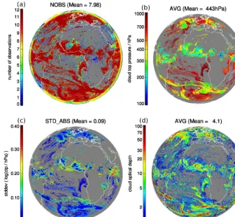
In Fig. 2 some basic statistics of the multi-algorithm en-semble are presented. In Fig. 2a we show the number of algorithms that detect a cloud and provide a CTP value for the observed satellite pixel. In general, the agreement of the cloud detection among the algorithms is good, in particular for the central parts of the cloud systems. However, at the edges of the cloud systems the cloud detection results differ. The ability to detect a cloud decreases when the sub-pixel cloud fraction and/or the COD decreases, see Fig. 2d show-ing the multi-algorithm ensemble average of the COD. There might also be overestimations of the cloud cover by some al-gorithms due to misinterpretation of aerosols or cloud free scenes as clouds. In particular, false cloud detection may oc-cur in case of large uncertainties in the surface albedo, emis-sivity and temperature.
Figure 1. Cloud top pressure (CTP) of ten SEVIRI algorithms for the 13 June 2008, 13:45 UTC. The mean CTP is calculated by averaging
Figure 2. Multi-algorithm ensemble statistics. Panel (a) displays the number of algorithms that provide a CTP value. Panel (b) shows the
multi-algorithm average of the cloud top pressure (CTP). Panel (c) shows the standard deviation of the log10(CTP). In Panel (b) and (c), values are shown for areas only, for which all retrievals detect clouds (common mask) to eliminate effects of different sample sizes. Panel (d) shows the multi-algorithm average of the cloud optical depth (not limited to the common mask). All images are for 13 June 2008, 12:00 UTC.
closest to fulfilling the common retrieval assumption of hor-izontal homogeneity; the vertical variation of the cloud tops is small and the optical depth is sufficiently high for a pre-cise retrieval of the CTP. In the extratropics there are some regions with large standard deviations: one band at 35◦S in the South Atlantic and another area in the North Atlantic near the Azores. The latter is located along the outer border of the cirrus associated with a warm front.
In Fig. 3 we investigate the latitudinal average of the CTP for the individual algorithms. The averages are calculated in two ways. In Fig. 3a and b, all available pixels provided by each of the algorithms are used in the averaging. This is called the individual cloud masks. For this case CTP statis-tics are influenced by both differences in the CTP retrieval methods and cloud detection. To exclude the effect of cloud detection, in Fig. 3c and d the CTP mean is computed using only those pixels that have a retrieved CTP value for all ten data sets. In the following, we refer to this filtering as the common cloud mask. The observed differences can be com-pletely attributed to characteristics of the CTP retrievals.
Looking at Fig. 3c and d, we notice that AWG, OCA, MFR, CMS and GSF tend to yield smaller CTPs, whereas MPF, DLR and LAR tend to produce higher CTPs compared to the average.
The differences between the data sets are larger for the individual than for the common cloud masks, as for the indi-vidual mask the samples are different and as the retrieval of cloud properties is often difficult for clouds that are hard to detect. In the tropics the multi-algorithm ensemble average, shown in black, is about 100 hPa higher for the individual than for the common cloud mask. This implies that above-average CTP values are retrieved for pixels that are not iden-tified as clouds by all algorithms. These are mainly broken clouds or optically thin cloud layers having an incorrectly great CTP (low CTH).
Figure 3. Latitudinal mean of the cloud top pressure of ten algorithms for 13 June 2008, 12:00–15:00 UTC. In panels (a) and (b) the original
data sets are used, whereas in panel (c) and (d) the data sets are reduced to observations, for which all ten retrievals detect a cloud and derive a CTP. The black line shows the average of all SEVIRI algorithms. In the lower panel (e) the relative standard deviations of the algorithm ensemble are shown.
most latitudes and better than 40 % in the tropics. The low-est standard deviations of about 15 % are south of 40◦S, at 20◦S, at 30◦N and north of 50◦N, in agreement with the
discussion of Fig. 2. Using the individual cloud masks in-stead of the common one, the standard deviations are 2 to 5 percentage points larger in the extratropics and about 10 to 15 percentage points larger in the tropics. This indicates that both the retrieval of the correct CTP as well as cloud detec-tion are most challenging for high thin cirrus clouds located mainly in the tropics. At the southernmost edge of the SE-VIRI disk, we also observe large standard deviations for the individual cloud masks. As the sun is close to the horizon in this region, not all algorithms provide a retrieval and the retrieval itself is difficult.
In Fig. 4 we investigate the histograms of the CTP, in Fig. 4a and b the individual mask and in Fig. 4c and d the common mask. All algorithms retrieve a comparable distri-bution of CTP values with two peaks: a first maximum be-tween the surface and 700 hPa representing boundary layer clouds and a second maximum between 300 and 200 hPa cor-responding to high cirrus and deep convective clouds. Mid-level clouds with CTP around 500 hPa occur less frequently.
The occurrence frequency of the boundary layer clouds is strongly reduced when reducing the data set to the common mask. Note the scale of the abscissa indicating the loss of data points when reducing the data sets to the common mask. The cloud frequency distributions with two maxima are in agreement with CTH measurements from MODIS. Chang and Li (2005a) found a distinct bimodal distribution of CTP peaking at 275 and 725 hPa for high and low clouds, thus leaving a minimum in cloud occurrence frequency in the middle troposphere.
Figure 4. Histograms of the cloud top pressure for 13 June 2008,
12:00–15:30 UTC. In panels (a) and (b) all retrieved values are taken into account, whereas in panels (c) and (d) only observations are taken into account, for which all ten retrievals detect a cloud and derive a CTP.
4 Comparison with CALIOP and CPR
To quantify the accuracy of the SEVIRI CTP/CTH retrievals, the SEVIRI data sets are validated against CALIOP and CPR retrieval products listed in Table 5. The CPR and CALIOP data sets have horizontal resolutions of 1.7 km and the 5.0 km, respectively.
The AVAC-S validation software (Bennartz et al., 2010) is applied to reproject these data sets on the SEVIRI grid. Furthermore, it takes care of the parallax correction for the SEVIRI viewing zenith angle. The AVAC-S software returns either the average of all CPR/CALIOP data points within one SEVIRI pixel or the data point nearest to the SEVIRI pixel center. In this paper averages over SEVIRI pixels are used everywhere. The CALIOP and CPR data are matched with the SEVIRI observations when the time shift is small-est. As SEVIRI scans one disk every 15 min, see Sect. 2.1, the maximum observation time difference is 7.5 min. In case a SEVIRI algorithm only provides CTP and not the CTH, CTP is transformed to CTH using pressure profiles as pro-vided in the ECMWF-AUX product of the CloudSat data
Table 5. List of CPR and CALIOP products used for the validation
of the SEVIRI algorithms.
Sensor Product Version
CPR 2B-GEOPROF 1.1
CPR 2B-CLDCLASS 5.3 CPR 2B-TAU_GRANULE 5.0 CALIOP CAL_LID_L1 3.01 CALIOP CAL_LID_L2_CLay 3.01 CALIOP CAL_LID_L2_VFM 3.01 Model ECMWF-AUX 5.2
processing center. In this section we concentrate our inves-tigation on the 13 June 2008, 12:00–15:30 UTC, as all ten SEVIRI data sets are available without gaps for this period. During this time the A-train satellite constellation passed the SEVIRI disk three times. The overpass numbers are 11317, 11318 and 11319.
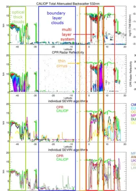
Figure 5 illustrates how the comparison of the SEVIRI, CALIOP and CPR retrievals is accomplished. The first and second panel show the CALIOP backscatter and CPR reflec-tivity signal, respectively. The CTHs detected by CALIOP and CPR are marked in green and red. In addition to the CTHs of the active instruments, the third and fourth panel show the CTHs derived by the individual SEVIRI algorithms. Large deviations indicate challenging conditions for CTH re-trievals. In Fig. 5 the CALIOP and CPR backscatter signals are used to qualitatively identify different cloud regimes: op-tically thick clouds, boundary layer clouds, multi-layer and optically thin clouds. For optically thick clouds (green area), the agreement between CALIOP, CPR and the SEVIRI CTHs is very good; the CALIOP CTH is slightly higher than the CPR and SEVIRI CTHs. For multi-layer clouds (red area) either the CPR or CALIOP sensor detect a second cloud layer. Between 0◦ and 5◦N all SEVIRI algorithms capture
the upper cloud layer. The deviations of the retrieval results are small on the right hand side, where the CPR backscatter signal indicates an optically thick upper cloud layer. The de-viations become larger with a decreasing CPR signal. In the orange regions CALIOP detects an optically thin cloud layer at about 16 km. The sensitivity of CPR is not sufficient to detect this layer; also, most SEVIRI algorithms cannot de-tect this cloud layer. The blue region marks the boundary layer clouds. The CPR does not detect these clouds as the ground clutter is larger than the cloud signal. Even though the CALIOP attenuated backscatter signal, see upper panel, indicates a fairly constant cloud top, some SEVIRI data sets deviate from the CALIOP CTH. All cloud regimes are dis-cussed in more detail in Sect. 4.2.
4.1 Overall statistics
Figure 5. Validation of the SEVIRI cloud top height (CTH) retrievals with CALIOP and CPR for 13 June 2008, 13:45 UTC or A-train
overpass 11318. In the first and second panel, the CALIOP backscatter profiles and the CPR reflectivity are shown together with the CTH derived from these instruments. In the third and fourth panel the CTHs derived by the ten SEVIRI algorithms are shown. The OCA algorithm additionally derives the CTH of a possible second cloud layer; this product is labeled as OCA2. Stars at the algorithm name indicate that these algorithms submitted CTP being converted to CTH. The colored boxes roughly indicate different cloud regimes being discussed in more detail in Sect. 4.2.
Here, the common mask refers to pixels, for which all SE-VIRI algorithms as well as CALIOP and CPR retrieve a CTP or CTH value, if not indicated differently. Therefore, the cloud detection abilities of all instruments influence the ex-tent of the common mask.
In Fig. 6 we investigate the effect of the common mask filter on the histogram of CTH. In Fig. 6a the histograms of the original CALIOP and CPR measurements are shown as dotted lines. It is possible to detect four relative cloud occur-rence maxima as a function of height. Due to different sensi-tivities of the instruments these maxima are detected at dif-ferent heights by CALIOP and CPR. For the individual mask the maximal cloud occurrence associated with the tropical tropopause layer (TTL) is detected at 16.5 and 13.5 km by CALIOP and CPR, respectively, the extratropical tropopause
at 10.75 and 10.25 km, the melting layer at 6.25 km and the boundary layer clouds at 1.25 km. The black line shows the mean of the SEVIRI algorithm histograms. For the individual mask the mean SEVIRI histogram shows a local maximum at 1.25 km for the boundary layer clouds. Other features are not well defined. A diffuse maximum at 11.75 km might be attributed to the TTL, the second at 9.5 km to the extratrop-ical tropopause. The maximum cloud occurrence at 6.25 km cannot be identified.
Figure 6. Histograms of the CTH for 13 June 2008, 12:00–15:30 UTC (A-train overpasses 11317–11319). Panel (a) shows the histograms
of the complete CALIOP and CPR data set and the average of the SEVIRI algorithm histograms as dotted lines. The histograms using the common mask filtering are shown as solid lines. In panels (b) and (c), the histograms of the individual algorithms are shown using the common mask filtering. For multi-layer cloud situations only the uppermost CTH is considered.
to classify it as cloud free. If one algorithm does so, the pixel is not included in the common mask. Another reason for the reduction of boundary layer cloud observations for the common mask is the low sensitivity of the CPR near the ground due to ground clutter. Therefore, CPR cannot detect all boundary layer clouds and, by definition, these pixels are excluded from the common mask.
For the common mask, it is still possible to identify the maxima for the TTL, extra-tropical tropopause and boundary layer in the CALIOP and CPR histograms. For the mean SE-VIRI histogram, the boundary layer cloud occurrence maxi-mum is clearly defined, but less pronounced for the SEVIRI retrieval average than for the active instrument results. This issue is discussed in more detail in Sect. 4.2.4. The maximum at 9.5 km is also detectable to some extent.
Figures 6b and c show the histograms of the individ-ual SEVIRI algorithms. There are some differences among the SEVIRI algorithms in reproducing the cloud occurrence maxima, for example, the cloud occurrence maxima of the boundary layer clouds of LAR, MFR and DLR are at higher altitudes than those of the other algorithms.
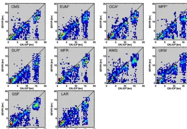
Figure 7 shows scatter plots of CTH detected by the indi-vidual SEVIRI algorithms against CALIOP measurements. Table 6 provides the corresponding differences of the mean values (bias), correlations, normalized standard deviations and root mean square differences (rmsd). Observations are taken into account, when all SEVIRI algorithms as well as the CALIOP retrieval provide CTH values. The scatter plots in Fig. 7 illustrate the capability of the different SEVIRI al-gorithms to retrieve CTH as a function of the CTH itself. In general, the majority of the scatter points are on the lower right side of the one-to-one line, meaning that the CTH re-trieved by the SEVIRI algorithm is lower than the CALIOP CTH. This is also evident from Table 6. On average all SE-VIRI CTHs are 1.05 km (AWG) to 2.50 km (DLR) lower
Table 6. Comparison with CALIOP for 13 June 2008, 12:00–
15:30 UTC. The table shows the difference of SEVIRI minus CALIOP of the mean CTH (bias), correlation between SEVIRI and CALIOP data set (corr), standard deviation of the single data sets divided by that of CALIOP (normalized standard deviation, nstd) and the root mean square difference (rmsd) between the SEVIRI data sets and CALIOP. Pixels are taken into account, for which all SEVIRI algorithms as well as the CALIOP retrieval provide CTH values. Bias and rmsd are given in meter. CALIOP derives a mean CTH of 7852 m with a standard deviation of 5374 m.
CALIOP, all clouds (2756 pixels)
group bias corr nstd rmsd
CMS −1668 0.850 0.808 3296 EUM −1683 0.833 0.772 3432 OCA −1496 0.888 0.833 2900 MPF −2468 0.781 0.747 4168 DLR −2502 0.816 0.739 4011 MFR −1483 0.863 0.788 3118 AWG −1049 0.896 0.856 2615 UKM −1463 0.864 0.828 3079 GSF −1310 0.900 0.773 2767 LAR −1743 0.766 0.743 3869
Figure 7. Scatter plots of the cloud top height SEVIRI data sets against the CALIOP data set for 13 June 2008, 12:00–15:30 UTC
(A-train overpasses 11317–11319). Most of the points are on the lower right side showing that the SEVIRI algorithms derive lower CTH than CALIOP.
Table 7. Same as Table 6, but for CPR. The mean of CPR
observa-tion is 6309 m and the standard deviaobserva-tion is 4306 m.
CPR, all clouds (2501 pixels)
group bias corr nstd rmsd
CMS −42 0.822 0.986 2552 EUM 10 0.858 0.949 2243 OCA 170 0.829 1.020 2553 MPF −734 0.868 0.926 2272 DLR −823 0.886 0.921 2165 MFR 74 0.821 0.967 2537 AWG 608 0.842 1.036 2541 UKM 180 0.851 1.015 2377 GSF 268 0.847 0.937 2333 LAR −19 0.855 0.920 2248
to CALIOP although some underestimated and a few over-estimated CTHs are seen. The underestimation of CTHs for clouds between 3 and 15 km is mainly caused by higher sen-sitivity of CALIOP to optically thin clouds compared to SE-VIRI. We discuss this issue in more detail in Sects. 4.2.2 and 4.2.3. For the boundary layer clouds with CALIOP CTHs between 0 and 3 km some scattering of the SEVIRI results is observed. EUM, MFR, GSF and LAR have a tendency to retrieve higher CTHs than CALIOP. This will be analyzed in Sect. 4.2.4.
Our results are in line with those from previous publica-tions. Holz et al. (2008) investigated the difference between the MODIS and CALIOP CTH in a similar way. They found that the MODIS CTH is 2.6±3.9 km lower than the CALIOP data set with 5 km horizontal resolution (same resolution as we use in this paper). They noted that the global CTH bias be-tween MODIS Collection 5 and CALIOP also depends on the CALIOP product resolution used. They found that CALIOP CTHs are only 1.4±2.9 km higher than MODIS Collection 5 CTHs when using the CALIOP 1 km layer products. For this resolution less CALIOP lidar shots are horizontally av-eraged and, therefore, the signal-to-noise ratio is lower than that of the 5 km product meaning the 1 km CALIOP product is less sensitive to optically thin clouds than the 5 km prod-uct. Hence, the higher spatial resolution is the fewer high clouds are detected by CALIOP and the CTH difference to data sets from passive sensors is smaller. Karlsson and Jo-hansson (2013) investigates the effect of the different cloud detection efficiency of the CALIOP 1 and 5 km product, too. They suggest a procedure to combine both CALIOP prod-ucts to obtain a data set for validation the CLARA-A1/PPS retrieval.
Figure 8. Same as Fig. 7, but for CPR. Pixels are taken into account, when all SEVIRI algorithms as well as the CPR retrieval provide CTH
values. In comparison to CALIOP more data points are close to the one-to-one line.
exceptions are OCA, AWG, UKM and GSF detecting mainly higher CTHs than the CPR. The magnitudes of the mean CTH differences between the SEVIRI data sets and CPR are smaller than 0.823 km for all SEVIRI data sets. The dif-ferences are sometimes positive and sometimes negative in contrast to the differences between the SEVIRI data sets and CALIOP being clearly negative for all algorithms.
Figure 9 shows a Taylor diagram (Taylor, 2001) of this evaluation. The radial coordinate is the standard deviation of the SEVIRI data set normalized with the standard deviation of the reference data set (CALIOP or CPR). The angle is the arcus cosine of the correlation coefficientRbetween the SEVIRI and the reference data sets. The reference point on thexaxis marks the point of an ideal agreement (correlation coefficient 1 and same standard deviation as the reference). The distance between the reference point and the marker of the SEVIRI data set is equal to the centered pattern root mean square difference (rmsd)E0
E0= 1
N
N X
n=1
[(sn−s)−(cn−c)]2 !1/2
, (13)
wheresn is the SEVIRI data,cn is the comparison data and
N is the total number of common data points.
The Taylor plot shows that the correlation coefficients for the comparisons against CALIOP and CPR are in the same range of roughly 0.77 to 0.90. The standard deviations of the SEVIRI data sets are more comparable to the CPR than to CALIOP as the latter is more sensitive to optically thin
Figure 9. Taylor diagram comparing the SEVIRI data sets with
Figure 10. Histograms of the CTH of thick, thin and multi-layer clouds for 13 June 2008, 12:00–15:30 UTC. Panel (a) shows the histograms
of the data as provided by the original CALIOP and CPR data sets as well as the mean of the histograms of the unfiltered SEVIRI data sets. In panel (b) only satellite pixels are taken into account for which all data sets provide a value. For multi-layer cloud situations only the uppermost CTH is considered.
clouds. UsingE0as the quality measurement, we see that the ranking of the algorithms depends on the reference data set, for example, the DLR algorithm has the lowest (best)E0with respect to the CPR, but a largeE0with respect to CALIOP. 4.2 Retrieval performance for different cloud regimes
In this section we investigate the uncertainties of CTH re-trievals for different cloud regimes: thick, thin and multi-layer clouds. We analyze how often these cloud regimes oc-cur and how they contribute to the overall deviations between the SEVIRI algorithms and the active sensors. In Sects. 4.2.1 to 4.2.3 there are separate discussions for each of these cloud regimes. In the last Sect. 4.2.4, we focus on clouds in the boundary layer, where possible ambiguities caused by the temperature profile make the conversion from CTT to CTH difficult.
First, we introduce the three cloud categories. We sepa-rate cloud cases into single layer and multi-layer clouds us-ing the CALIOP product Number of Layers Found. The sin-gle layer category is further subdivided into optically thin and thick clouds. Clouds with a CALIOP column cloud opti-cal depth at 532 nmτcal<3 are defined as thin and clouds with τcal≥3 as thick. Table 8 lists our cloud categories. We choose a threshold of 3 to be comparable to the ISCCP cloud classification (Rossow et al., 1985; Rossow and Schif-fer, 1999).
Figure 10 shows the histograms of the three cloud cat-egories for 13 June 2008, 12:00–15:30 UTC. Figure 10a shows the histograms of the unfiltered data sets. The same layers with increased cloud occurrence are observed as in Fig. 6, but in this figure information about the cloud
Table 8. Definition of three cloud categories investigated in
Sect. 4.2. Single and multi-layer clouds are separated by the CALIOP product Number of Layers Found (NLF). Single layer clouds are further subdivided into optically thin and thick clouds using the CALIOP column cloud optical depth at 532 nmτcal.
Cloud category Criteria
Single layer thin cloud NLF=1 andτcal<3 Single layer thick cloud NLF=1 andτcal≥3 Multi-layer clouds NLF>1
categories is additionally provided. In the TTL at 15 to 16 km, thin and multi-layer clouds are detected by CALIOP. The CPR captures mainly multi-layer clouds and some of the thin clouds at about 13 km. At the extratropical tropopause at 11 km both sensors detect primarily multi-layer clouds, at 6.5 km thin clouds and multi-layer are detected, and in the boundary layer mainly thin and some thick clouds are observed. The high occurrence of thin clouds detected by CALIOP in the boundary layer may be explained by the av-eraging of CALIOP retrievals over the area of one SEVIRI pixel. The frequent occurrence of optically thin clouds in the boundary layers detected by SEVIRI can partly be caused by misinterpretation of broken clouds, being inhomogeneous on a sub-pixel scale, as thin clouds.
sets. The mean SEVIRI histogram shows maxima of thin and thick cloud occurrences in the boundary layer, but these are less sharp than the corresponding maxima of CALIOP and CPR at 1.25 km. As primarily single layer clouds are domi-nant in this region, we conclude that the different shapes of the peak are not due to other cloud layers above the boundary layer clouds, but have to be explained by other reasons like for instance retrieval ambiguities due to temperature inver-sions, see Sect. 4.2.4. The mean SEVIRI multi-layer CTHs are more or less evenly distributed between 2 and 13 km.
Tables 9 and 10 provide the same statistics as Tables 6 and 7 but are separated into thick, thin and multi-layer clouds. For thick single layer clouds the correlation coefficients are usually greater than 0.95 in comparison to both active instru-ments. The mean differences to CALIOP and CPR are only a few hundred of meters for most algorithms, but LAR over-estimates the CTH compared to both reference data sets by more than 600 m. The root mean square deviations are gen-erally about 1 km.
For optically thin clouds the CTH differences tend to be-come negative. In particular MPF and DLR retrieve CTHs that are about 1 km lower than CALIOP and about 600 m lower than CPR. Most of the correlation coefficients are above 0.92. The root mean square deviations are between 1.5 and 2.5 km.
The lowest correlations and largest biases are observed for multi-layer clouds. The correlation coefficients are between 0.59 and 0.83 in comparison to CALIOP and between 0.64 and 0.79 in comparison to CPR. The mean SEVIRI CTHs are 2.1 km to 4.4 km lower than the mean CALIOP CTH. The biases in comparison to CPR are smaller. We find that MPF and DLR detect average CTHs more than 1 km lower than CPR, whereas the CTH of AWG is 982 m higher than CPR.
These results are summarized in the Taylor diagrams for the different cloud categories, see Fig. 11. For optically thick clouds the performance of the SEVIRI retrievals compared to CPR and CALIOP are very similar to each other. The same is true for optically thin clouds, but for multi-layered clouds, the locations of the algorithms in the Taylor plot are different comparing the CALIOP and CPR diagrams.
Figure 12 shows the mean difference and root mean square difference (rmsd) of the CTH between the SEVIRI algo-rithms and the active sensors as a function of the CALIOP COD τcal. Taking all clouds into account, see upper row of Fig. 12, the SEVIRI algorithms retrieve CTHs that are about 1 km lower than the CALIOP CTH for τcal>2. For smallerτcalthe SEVIRI CTHs are about 2 to 4 km lower than CALIOP depending on the algorithm. Forτcal>2 the aver-age rmsd is about 3 km and increases to 5 km for smallerτcal. The second row shows the same statistics, but for sin-gle layer clouds only. Forτcal>2 the bias between the SE-VIRI and CALIOP algorithms vanishes and the rmsd is about 1 km. For smaller τcal the bias and rmsd increase to up to 2 km and 3 km, respectively.
The third row of Fig. 12 shows the results for multi-layer clouds. The bias and rmsd do not systematically depend on
τcalrepresenting the COD of all cloud layers up to the COD where the lidar signal is saturated. The bias is about 3 to 4 km and the rmsd is about 4 to 5 km with respect to CALIOP.
We note that the bias is larger for the multi-layer clouds than for the thin single layer clouds. One reason for this is the assumption of a single layer cloud made by all SEVIRI retrieval algorithms except OCA and AWG. In theory, radi-ance ratioing can account for the semi-transparency of opti-cally thin cloud layers and, therefore, can retrieve a correct CTH with its associated uncertainty (in practice this is not always the case). With a second layer underneath and the assumption of a single layer cloud, the correct CTH cannot be retrieved by definition. The best possible retrieval solu-tion for this case is a CTH lying somewhere between the two cloud layers. Hence, there is a direct reason for a distinct low bias of the CTHs retrieved for the upper cloud layer. A sec-ond reason is the reduction of cloud cases by the common mask. For the single layer category a significant fraction of thin cirrus clouds are not captured by at least one SEVIRI algorithm and, therefore, are not included in the common mask data set. Looking at Fig. 10a, we observe that espe-cially the thin clouds at about 15 km are often excluded by this procedure. On the other hand, for multi-layer clouds the lower cloud layer increases the chance of cloud detection, even though the uppermost cloud layer might be optically very thin. Therefore, a large fraction of multi-layer observa-tions are still included in the common mask data set.
The second and fourth columns of Fig. 12 show the same comparison, but for CPR data. Considering all clouds, the mean SEVIRI CTH is close to the CPR CTH for allτcal. The rmsd is about 2 km forτcal>1.5 and increases up to 4 km for smallerτcal. For single layer clouds the biases are still small, only MPF shows a tendency to underestimate the CTH for optically thin clouds. The rmsd of single layer clouds is about 50 % of the rmsd of all clouds. The CTH bias with respect to CPR of multi-layer clouds shows no clear dependency on
τcal. For multi-layer clouds, the mean bias is around 0 km and the rmsd is between 2 and 4 km, but there are individual characteristics of the SEVIRI algorithms.
4.2.1 Discussion for optically thick clouds
To explain the CTH differences between SEVIRI and the ref-erence data, it is important to take the different sensitivities of the satellite sensors into account. CALIOP, being the most sensitive instrument, see Sect. 2.1, is able to detect the CTH close to the physical one. CPR, on the contrary, is less sen-sitive to clouds with small optical depths. Therefore, it is ex-pected that the CPR CTH is generally below the CALIOP counterpart.
Table 9. Same as Table 6, but for three cloud regimes: thick, thin and multi-layer clouds. For multi-layer clouds the statistics are given with
respect to the uppermost cloud layer. The mean CTHs observed by CALIOP are 4000, 5496 and 11014 m and the standard deviations are 3497, 4784 and 4461 m for thick, thin and multi-layer clouds, respectively.
Thick clouds (500 pixels) Thin clouds (968 pixels) Multi-layer clouds (1306 pixels)
group bias corr nstd rmsd bias corr nstd rmsd bias corr nstd rmsd
CMS 6 0.959 0.914 1003 −596 0.928 0.888 1890 −3098 0.721 0.917 4464 EUM 203 0.959 0.914 1020 −513 0.925 0.855 1917 −3267 0.689 0.876 4670 OCA −117 0.969 0.945 873 −643 0.941 0.893 1762 −2651 0.783 0.920 3885 MPF −196 0.981 0.918 745 −1068 0.884 0.824 2490 −4359 0.642 0.881 5641 DLR −257 0.967 0.889 970 −1039 0.924 0.863 2120 −4435 0.698 0.841 5503 MFR 154 0.954 0.876 1095 −393 0.928 0.859 1852 −2923 0.755 0.895 4182 AWG 140 0.957 1.017 1040 −208 0.944 0.952 1586 −2128 0.794 0.897 3475 UKM 75 0.952 1.014 1090 −517 0.923 0.946 1917 −2756 0.744 0.869 4095 GSF 334 0.972 0.905 914 −159 0.943 0.833 1688 −2779 0.834 0.874 3715 LAR 624 0.947 0.979 1291 −394 0.899 0.830 2154 −3643 0.591 0.854 5253
Table 10. Same as Table 9, but for CPR. For clarification the same criteria using CALIOP products are applied for separation of the cloud
regimes. The mean CTHs observed by CPR are 4289, 5208 and 7919 m and the standard deviations are 3480, 4236 and 4050 m for thick, thin and multi-layer clouds, respectively.
Thick clouds (445 pixels) Thin clouds (918 pixels) Multi-layer clouds (1157 pixels)
group bias corr nstd rmsd bias corr nstd rmsd bias corr nstd rmsd
CMS 38 0.959 0.928 987 −127 0.929 0.990 1593 −28 0.639 0.992 3425 EUM 182 0.966 0.940 915 −66 0.926 0.956 1602 −16 0.724 0.936 2921 OCA −99 0.968 0.970 874 −216 0.930 1.000 1595 551 0.646 0.979 3414 MPF −177 0.981 0.940 706 −605 0.920 0.928 1764 −1067 0.767 0.957 2911 DLR −284 0.969 0.916 927 −644 0.946 0.975 1516 −1192 0.785 0.916 2828 MFR 128 0.953 0.901 1071 10 0.924 0.966 1633 81 0.643 0.973 3376 AWG 195 0.964 1.038 984 291 0.923 1.050 1741 982 0.675 0.953 3340 UKM 86 0.958 1.036 1035 −59 0.922 1.054 1730 363 0.702 0.941 3062 GSF 311 0.979 0.930 791 244 0.928 0.926 1596 250 0.694 0.932 3078 LAR 639 0.952 1.005 1257 43 0.915 0.930 1705 −345 0.743 0.923 2828
radiance at the top of atmosphere Iν can be derived by
in-tegration of the Schwarzschild equation (Sherwood et al., 2004):
Iν= ∞ Z
0
Bν(τ )e−τdτ. (14)
By assuming that the Planck radiation Bν(τ ) varies
lin-early with the CODτ, it may be inferred from this equation that Iν=Bν(τ=1)which means that the CTT (and
subse-quently the CTH) derived from the measured radiance Iν
is representative of a level at an optical depth of τ=1 be-low the actual CTH. This is not to say that it is not pos-sible to detect clouds with an optical depth smaller than 1 with passive imagers: the detection limits are estimated to be about 0.1 to 0.3 depending on the algorithm. Taking scatter-ing into account, Sherwood et al. (2004) states that for opti-cally thick clouds the 10.8 µm signal seen by passive imagers corresponds to the temperature at a level located at an optical
depth of 1 to 3 measured from the cloud top. The geometric height of this level depends on the ice or liquid water content and effective particle size in the upper layers of the cloud (Minnis et al., 2008a). Because water contents are typically much smaller for ice clouds as compared to liquid clouds, the difference between the effective and physical top heights of the clouds is expected to be much smaller for liquid than for ice clouds.
Figure 11. Taylor diagram for CALIOP (left) and CPR (right). Similar to Fig. 9, but the statistics are calculated separately for optically thick
(τcal≥3) and thin (τcal<3) single layer clouds as well as for multi-layer clouds.
Figure 12. Differences and root mean square deviations (rmsd) of the CTH between the SEVIRI and CALIOP and CPR in dependence of the
Table 11. Same as Table 6, but for clouds with a CALIOP CTH
smaller than 3.25 km only. Pixels are taken into account, for which all SEVIRI algorithms as well as the CALIOP retrieval pro-vide CTH values. This comparison is for 13 June 2008, 12:00– 15:30 UTC. The mean CTH retrieved from CALIOP is 1806 m and the standard deviation is 661 m.
CALIOP, low clouds (819 pixels)
group bias corr nstd rmsd
CMS 139 0.400 1.884 1162 EUM 345 0.326 1.549 1078 OCA −41 0.605 1.387 738 MPF 51 0.590 1.194 668 DLR −20 0.255 1.174 882 MFR 458 0.322 1.858 1277 AWG 32 0.395 1.682 1046 UKM 44 0.479 2.029 1178 GSF 621 0.567 1.791 1156 LAR 587 0.310 1.355 1103
MODIS collection 5 agrees with lidar measurements within 50 hPa or 1 km for high, optically thin cirrus and mid-level water clouds (both single layer). Sherwood et al. (2004) observed that the CTH of deep convective clouds derived from GOES-8 observations is 1 to 2 km below measure-ments of the airborne Cloud Physics Lidar (CPL) during the CRYSTAL-FACE campaign.
Looking at the statistics for optically thick clouds in Ta-ble 9, we observe that the mean SEVIRI CTH is lower than that of CALIOP for OCA, MPF and DLR. But for the other algorithms the mean CTH is higher than CALIOP. Especially LAR overestimates the CTH for thick clouds mainly as a re-sult of overestimating low cloud heights, see Tables 11 and 12.
All SEVIRI retrievals aim for a small total CTH bias. So it is possible that an algorithm overestimates the CTH for thick clouds so that the negative bias of optically thin and multi-layer clouds is partly balanced in the overall bias. There are also other possible reasons for the observed differences be-tween the CTH retrievals of passive and active sensors, such as different viewing geometries and different fields of view as well as the effect of the cloud top structure (Dong et al., 2008). These uncertainties may create underestimation as well as overestimation, hence, they partly compensate each other in their effect on the mean bias, whereas the differences between the effective and physical CTH does not.
4.2.2 Discussion for optically thin clouds
The retrieval of the CTH is more complicated for semi-transparent than for opaque cloud situations. The ther-mal emission from the surface and the atmosphere below the cloud contribute to the observed thermal radiance, see Eq. (5). Therefore, the cloud emissivity, the emission of the
Table 12. Same as Table 11, but for CPR. For clarification, the
iden-tification of low clouds is done with the CALIOP CTH. Pixels are taken into account, for which all SEVIRI algorithms as well as the CALIOP and CPR retrieval provide CTH values. The mean CTH retrieved by CPR is 1996 m and the standard deviation is 726 m.
CPR, low clouds (726 pixels)
group bias corr nstd rmsd
CMS 119 0.380 1.783 1225 EUM 274 0.381 1.526 1102 OCA −123 0.621 1.368 794 MPF −17 0.638 1.046 632 DLR −155 0.295 1.065 904 MFR 338 0.326 1.759 1291 AWG 46 0.433 1.682 1118 UKM −22 0.467 1.818 1171 GSF 534 0.547 1.683 1155 LAR 507 0.343 1.342 1116
surface and atmosphere below the cloud influence the radia-tive transfer. For the simultaneous retrieval of CTH and the cloud emissivity, it is necessary to use at least two thermal channels. It is expected that the uncertainty of the retrieved CTH increases with decreasing emissivity of the cloud, as the difference between clear and cloudy sky radianceIν−Iνclr
used for the CTH retrieval becomes small, see Eq. (12). Un-certainties arise not only from the assumptions made for the water vapor profile as well as the surface temperature and emissivity, but also from instrument noise, spectral response function errors and radiative model approximations (Menzel et al., 2008).
Smith and Platt (1978) noted that on average the CTH de-rived by CO2 slicing is located at the height corresponding to half of the optical thickness for optically thin clouds. Dur-ing the validation of the SEVIRI retrievals, we noticed cases of optically thin clouds, where retrieved SEVIRI CTHs lie far below the cloud’s mid-level height and sometimes even below the cloud base. This has also been observed in other studies. It was found that CTH differences between passive instruments and lidar retrievals may be as large as 3 km for thin cirrus clouds, in particular for geometrically thick but tenuous clouds (Holz et al., 2006, 2008; Chang et al., 2010). This issue seems to affect many algorithms and needs to be researched in more detail.
4.2.3 Discussion for multi-layer clouds