www.atmos-meas-tech.net/8/3107/2015/ doi:10.5194/amt-8-3107-2015
© Author(s) 2015. CC Attribution 3.0 License.
GOMOS bright limb ozone data set
S. Tukiainen1, E. Kyrölä1, J. Tamminen1, J. Kujanpää1, and L. Blanot2 1Finnish Meteorological Institute, Earth Observation Unit, Helsinki, Finland 2ACRI-ST, Sophia Antipolis, France
Correspondence to: S. Tukiainen ([email protected])
Received: 5 December 2014 – Published in Atmos. Meas. Tech. Discuss.: 27 January 2015 Revised: 26 June 2015 – Accepted: 10 July 2015 – Published: 5 August 2015
Abstract. We have created a daytime ozone profile data set from the measurements of the Global Ozone Monitoring by Occultation of Stars (GOMOS) instrument on board the En-visat satellite. This so-called GOMOS bright limb (GBL) data set contains ∼358 000 stratospheric daytime ozone profiles measured by GOMOS in 2002–2012. The GBL data set complements the widely used GOMOS nighttime data based on stellar occultation measurements. The GBL data set is based on the GOMOS daytime occultations but in-stead of the transmitted star light we use limb-scattered so-lar light. The ozone profiles retrieved from these radiance spectra cover the 18–60 km altitude range and have approxi-mately 2–3 km vertical resolution. We show that these pro-files are generally in better than 10 % agreement with the NDACC (Network for the Detection of Atmospheric Com-position Change) ozonesonde profiles and with the GOMOS nighttime, MLS (Microwave Limb Sounder), and OSIRIS (Optical Spectrograph and InfraRed Imager System) satellite measurements. However, there is a 10–13 % negative bias at 40 km altitude and a 10–50 % positive bias at 50 km for so-lar zenith angles>75◦. These biases are most likely caused by stray light which is difficult to characterize and to remove entirely from the measured spectra. Nevertheless, the GBL data set approximately doubles the amount of useful GO-MOS ozone profiles and improves coverage of the summer pole.
1 Introduction
The GOMOS (Global Ozone Monitoring by Occultation of Stars) instrument on board the Envisat satellite uses the stel-lar occultation technique for monitoring ozone and other
trace gases in the middle atmosphere (Bertaux et al., 2010). Envisat operated from 2002 to 2012 and during that time GOMOS measured altogether around 880 000 occultations. While the GOMOS nighttime ozone profiles have generally less than 5 % bias in the stratosphere (Meijer et al., 2004; van Gijsel et al., 2010; Kyrölä et al., 2013), the majority of the daytime occultation profiles are poor due to weak sig-nal to noise ratio (Verronen et al., 2007). For this reason, the GOMOS daytime occultation profiles have not been used in scientific studies.
To improve the GOMOS daytime ozone profiles, Taha et al. (2008) suggested using atmospheric limb radiance of scattered sunlight instead of star spectra for the daytime re-trievals. GOMOS measured limb radiances above and below the occulting star using a separate optical path so that the star and the limb contributions can be distinguished from each other (see Bertaux et al., 2010, for a detailed descrip-tion of the instrument). In principle, the subtracdescrip-tion of the pure limb signal from the central band, containing both the star and the limb contribution, should produce an uncontam-inated star spectrum. However, it seems that this removal leads to large and poorly understood uncertainties in the day-time transmission spectra, ruining the operational GOMOS occultation retrieval that works fine for the nighttime data. In their study, Taha et al. (2008) used an optimal-estimation-based method to retrieve ozone from the limb scatter radi-ances and reported up to 10–15 % agreement with the refer-ence data from Stratospheric Aerosol and Gas Experiment II (SAGE II) between 25–53 km. The authors retrieved separate ozone profiles from both bands (upper/lower) and obtained consistent results.
retrieving ozone profiles from the GOMOS limb scattered radiances, or GOMOS bright limb (GBL) measurements as they are referred to from now on. This paper is a continuation of that study. We have processed all GOMOS daytime mea-surements and in this study we estimate the quality of this novel data set. We also tested the sensitivity of the retrieval method to the selected spectral band and decided to use the lower band radiance to process the GBL data set. Another important decision is the choice of the stray light removal method (GOMOS daytime radiances are badly contaminated by stray light). In this work, we adapted a simple method that estimates the average stray light from the high tangent altitude GOMOS spectra. The structure of this paper is as follows. In Sect. 2 we describe the retrieval method, test its sensitivity, and explain some general aspects of the GOMOS daytime data. In Sect. 3 we describe the correlative data sets used to validate the retrieved GBL ozone profiles, present the comparison method, and show the results of the comparisons. In Sect. 4 we conclude our study and discuss the results.
2 GOMOS bright limb data
The GOMOS bright limb data set consists of ∼358 000 limb-scattered radiance spectra measured around 10:00 LT between March 2002 and April 2012, from the launch of En-visat to the communication failure that stopped the mission. From these measurements we have retrieved vertical ozone profiles in the 18–60 km altitude range. The retrieved profiles have approximately 2–3 km vertical resolution. The data are processed using the ESA IPF (Instrument Processing Facil-ity) Level 1 version 6.01 and the current GBL Level 2 ver-sion 1.2. The Level 2 retrieval scheme is based on Tukiainen et al. (2011) with a few modifications. We describe the re-trieval method briefly below.
One GOMOS limb “scan” includes typically 120–140 in-dividual radiance measurements at different tangent heights. Since GOMOS records two separate radiance spectra at each tangent height, above and below the central band (which col-lects the combined star and limb signal), there are actually twice as many spectra. The GBL data set was processed us-ing the lower band radiances but the upper band, or possibly a combination of both bands, could be used as well. The up-per and lower band radiances are separated by around 1.5 km in tangent height. One particular advantage of GOMOS is that the tangent height registration is very accurate: on the or-der of 30 m (Bertaux et al., 2010). Stars are point sources and their positions are well known. Because the GOMOS central band always follows the occulting star, the uncertainty in the tangent height, which is often a significant problem in limb scatter satellite observations, is a negligible issue in the GO-MOS retrievals (Tamminen et al., 2010).
In the retrieval, the model atmosphere is discretized into homogeneous layers whose center point heights match the tangent heights of the corresponding radiance measurements.
We use an onion peeling retrieval approach to estimate trace gas densities, starting from the topmost layer used in the re-trieval (at∼60 km) and proceeding layer by layer towards the bottom layer (at∼18 km). At each layer, we minimize the cost function
χ2(z)= [H(λ, z)−M(λ, z)]C−1[H(λ, z)
−M(λ, z)]T, (1)
whereMis the (stray-light-corrected) radiance measurement at layerzand a function of wavelengthλ. It is normalized with the first measurement below 47 km of the same scan. The diagonal uncertainty covariance matrix C includes the standard deviation of the measurement error. Currently, no modeling error is assumed, see details in Tukiainen et al. (2011). The modeled radiance,
H(λ, z)=R(λ, z)Iss(λ, z,ρ)
Iref(λ)
, (2)
consists of the modeled total to single scattering ratioR, cal-culated in advance as a look-up table, and the single scat-tering radianceIss divided by the modeled reference spec-trumIref.Rdepends only weakly on the actual trace gas pro-files, allowing us to keep it fixed during the fitting process. With this assumption, we only need to solve the single scat-tering radianceIsswhich can be effectively calculated using simple numerical integration. The reference spectrumIrefis estimated using neutral air density from the ECMWF (Eu-ropean Centre for Medium-Range Weather Forecasts) model analysis data (MSIS-90 climatology above 1 hPa) and clima-tological trace gas profiles.
The retrieved gas densities, ρ, include ozone, aerosols, and neutral air. NO2 is taken from a climatology and kept fixed. The NO2 climatology is based on OSIRIS (Optical Spectrograph and InfraRed Imager System) data (Tukiainen et al., 2008). Aerosol scattering is modeled with the Henyey– Greenstein phase function and aerosol extinction is modeled with the Ångströmλ−1law. Rayleigh scattering is assumed for neutral air. The minimization ofχ2in Eq. (1) is done with the Levenberg–Marquardt method. The error covariance ma-trix of the retrieved densities is estimated at the minimum assuming Gaussian posteriors:
Cr=(J0J)−1
χ2
(n−p), (3)
0 5 10 15 20
25 30 35 40 45 50 55
Relative error [%]
Altitude [km]
0 0.5 1 1.5
Reduced χ2
Figure 1. Interquartile range of the relative error (left) and reduced χ2(right). Data from the tropics, year 2004.
error bars for the profiles. In theory, the reduced χ2should be unity but the averageχ2 of GBL is around 0.5 between 20 and 45 km and the scaling is needed (Fig. 1, right panel). The GBLχ2values of less than unity indicate some issue in the measurement error characterization.
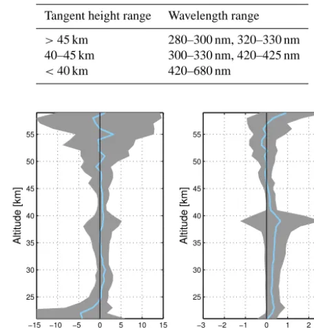
GOMOS daytime radiances are significantly contaminated by stray light, especially at visible wavelengths and at high tangent altitudes. For example, below 40 km at 500 nm the stray light accounts roughly for a few percents of the signal but already several 10 % at 60 km. We remove the stray light by calculating the average spectrum above 100 km and by subtracting this constant spectrum from each tangent height. The removal is done independently for each scan. This ap-proach ignores a possible altitude dependence of the stray light but, on the other hand, is a simple and robust method. To avoid using the most corrupted wavelength regions, we use three different sets of retrieval wavelengths depending on the tangent height (Table 1). This reduces bias due to inconsis-tencies in the GOMOS spectra but also introduces a disconti-nuity at 40 km where we start using only visible wavelengths. We reduce the discontinuity by scaling the amount of stray light (at layers below 40 km) by an iteratively found constant factor, requiring that the ozone profile remains smooth in the 40 km transition.
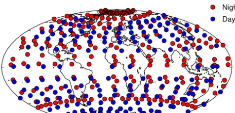
We tested the sensitivity of the GBL ozone to the two important assumptions in the retrieval: the choice of the charge-coupled device (CCD) band of the spectrometer (up-per or lower) and the stray light correction method. The test data included 10 orbits (142 scans) from 1 April 2004. The two available CCD bands yield ozone profiles within 1 % (Fig. 2 left panel). The difference is calculated, after linear interpolation in altitude, as (upper–lower)/lower×100 (%). This figure visualizes the propagation of the random mea-surement error in the GOMOS limb retrieval. For the stray light correction, we tested two methods: the con-strained extrapolation method introduced in Tukiainen et al. (2011) and the simple average method described above. The difference in the retrieved ozone profiles is below 1 %
Table 1. Wavelength ranges used in the retrieval.
Tangent height range Wavelength range
>45 km 280–300 nm, 320–330 nm
40–45 km 300–330 nm, 420–425 nm
<40 km 420–680 nm
−3 −2 −1 0 1 2 3 25
30 35 40 45 50 55
Altitude [km]
Difference [%]
−15 −10 −5 0 5 10 15 25
30 35 40 45 50 55
Altitude [km]
Difference [%]
Figure 2. Sensitivity of GBL ozone profile to CCD band (left) and stray light correction method (right). Shown are the mean (solid line) and standard deviation (shaded area) of the relative individ-ual differences of the retrieved profiles in both cases. See text for details.
(Fig. 2 right panel). The difference is defined as (average– constrained)/constrained×100 (%). As both methods pro-duce, at least in this case, almost identical ozone profiles it is probably better to use the average method because of its simplicity.
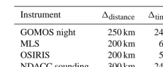
Each GBL Level 2 file contains geolocation information, ECMWF model values for the temperature and density, a fixed NO2profile (from the OSIRIS climatology), and resid-uals of the fit. Densities and error estimates are provided for the three simultaneously retrieved species: ozone, aerosols, and neutral air. In this paper we show only the results related to the ozone profiles. Figure 3 shows the number of GBL profiles and GOMOS nighttime occultation profiles during the whole Envisat mission. The GBL data set roughly dou-bles the amount of useful GOMOS ozone profiles. Figure 4 shows a typical 1-day coverage of GOMOS day and night measurements, and Fig. 5 shows the number of GBL pro-files during 1-year (2004) as a function of latitude. The GBL data complements the night occultations in the tropics and mid latitudes and furthermore expands the global coverage towards the summer pole.
2003 2004 2005 2006 2007 2008 2009 2010 2011 2012 0
1000 2000 3000
Year
Number of measurements
night + day day
Figure 3. Number of GOMOS nighttime and GBL measurements (weekly).
Night
Day
Figure 4. Typical 1-day coverage of GOMOS night occultations (red) and GBL (blue). Data from 15 December 2004.
the daytime data from the star number 175. As practically always, the shapes of the day occultation profiles are signif-icantly different than the shapes of the GBL and night oc-cultation profiles. The huge fluctuations and large negative values seen in the day occultation profiles are not realistic. At least in the stratosphere, the quality of the day occultation profiles is clearly inferior to the GBL and GOMOS nighttime data.
3 Correlative data sets
First, we compared the retrieved GBL ozone profiles against NDACC (Network for the Detection of Atmo-spheric Composition Change) balloon-borne ozonesonde measurements. The NDACC data can be downloaded from http://www.ndacc.org and the stations that were used in the comparison are listed in Table 2. While ozonesondes typi-cally reach only about 30–35 km altitude, they measure tro-pospheric and lower stratospheric ozone with very good ver-tical resolution. Also, in general, the accuracy and precision of ozonesondes is at least as good as satellite measurements. To validate the GBL profiles also for altitudes above 35 km, we compared the GBL data against satellite measure-ments from the GOMOS nighttime occultations, MLS (Mi-crowave Limb Sounder) on EOS (Earth Observing System) Aura (Waters et al., 2006), and OSIRIS on Odin (Llewellyn et al., 2004; McLinden et al., 2012).
Month
Latitude [
o ]
1 2 3 4 5 6 7 8 9 10 11 12
−90 −60 −30 0 30 60 90
Number of measurements
0 100 200 300 400 500
Figure 5. Number of GBL measurements as a function of latitude and time during 2004.
−5 0 5 10 15
20 30 40 50 60 70 80 90 100 110
Ozone mixing ratio [ppmv]
Altitude [km]
Day occultation Night occultation GBL
Figure 6. Example of the vertical distribution of ozone from the GOMOS night/day occultations and GBL. Data from January 2005, latitude 35◦N (zonal medians and interquartile ranges).
For GOMOS night occultations, we used the latest Level 2 version 6 data. Because the occultation retrieval from cool and weak stars is also difficult due to low signal to noise ratio and often results in mediocre nighttime occultation profiles (see the data disclaimer ESA, 2012), we screened out these “bad star” profiles from the comparison.
Table 2. NDACC stations that were used for different latitude zones.
60–90◦N 30–60◦N 30◦S–30◦N 30–60◦S 60–90◦S
Scoresby Sound Obs. de Haute Provence Paramaribo Lauder Dumont d’Urville
Ny Ålesund Hohenpeißenberg Iza´na Neumayer
Sodankylä Legionowo Natal
Summit De Bilt
Eureka Boulder
Alert Wallops
Thule Prague
1 hPa) and the MSIS-90 climatology (above 1 hPa), which are included in the GOMOS Level 1 data. It is convenient to use the neutral density data from the Level 1 product, espe-cially as the ECMWF data below 1 hPa (∼50 km) are gen-erally very accurate (errors of less than 1 %). The MSIS-90 climatology, merged with the ECMWF data, is less accurate though. Nevertheless, we estimate that the accuracy of the GOMOS Level 1 neutral air product between 50 and 60 km is still better than approximately 5 %.
OSIRIS is a UV/visible spectrograph, including a near-infrared imager, on board the Odin satellite. OSIRIS sures the atmosphere using the limb scatter technique, mea-suring scattered sunlight and scanning Earth’s limb between
∼10 and 100 km. In this work, we have used two dif-ferent OSIRIS ozone profile products. The University of Saskatchewan’s OSIRIS ozone product is retrieved from OSIRIS data using the SaskMART (Saskatchewan mul-tiplicative algebraic reconstruction technique; Degenstein et al., 2009). The product has been the target in several vali-dation studies (e.g., Adams et al., 2012, 2013). In this study we use the version 5.07 of these data. The Finnish Meteoro-logical Institute’s (FMI) OSIRIS ozone product is retrieved using the modified onion peeling method (Tukiainen et al., 2008), which is similar to the method used in this work. The present version is 3.2. The two available OSIRIS ozone prod-ucts agree with each other within a couple of percents. 3.1 Comparison method
For each co-located profile pair we calculated the difference as
1=XGBL−Xref
Xref
×100(%), (4)
where XGBL is a GBL profile and Xref is a reference (NDACC, GOMOS night, MLS or OSIRIS) profile. The coincidence criteria for each instrument are shown in Ta-ble 3. To estimate the bias against GOMOS night, MLS and OSIRIS, we calculated the median of the individual rela-tive differences using 10◦latitude zones between 70◦S and 70◦N. With the NDACC soundings we used only six lati-tude zones (see Table 2) because the latilati-tude coverage of the NDACC sounding stations is much sparser than of the polar
Table 3. Coincidence criteria for the GBL and correlative measure-ments.
Instrument 1distance 1time
GOMOS night 250 km 24 h
MLS 200 km 6 h
OSIRIS 200 km 5 h
NDACC sounding 300 km 24 h
orbiting satellites especially in the Southern Hemisphere. We also calculated the bias against GOMOS night occultations as a function of solar zenith angle.
In the median calculation, we used coincidences from all overlapping years. Possible year-to-year differences due to e.g., aging of the instruments were found insignificant (a few percents with no clear pattern) compared to the other sources of bias. In addition, the vertical resolutions of the four different satellite ozone products are similar (2–3 km for GBL, GOMOS night, and OSIRIS, and∼3 km for MLS). Therefore, these profiles were compared without any verti-cal smoothing. The vertiverti-cal resolution of GBL is determined by the field of view of GOMOS and the movement of the satellite during the measurement. These lead to an∼2 km theoretical resolution in the GBL product, which is further lowered to∼2–3 km due to the retrieval method, accord-ing to our estimate. In the GOMOS occultation retrieval, the resolution is fixed to 2–3 km (depending on the altitude) us-ing the Tikhonov regularization and target resolution tech-nique (Tamminen et al., 2010). The vertical resolutions of the OSIRIS and MLS ozone products are very close to the GO-MOS resolutions and the marginal resolution differences do not seem to cause any notable issues in the comparisons. The NDACC ozonesonde profiles, which have significantly bet-ter vertical resolution, were smoothed to the approximately same resolution with the satellite products using a Gaussian filter.
−30 −20 −10 0 10 20 30 20 25 30 35 60−90N 34 240 366 479 567 608 611 609 599 587 572 541 508 426 296 165 77 Altitude [km]
−30 −20 −10 0 10 20 30
20 25 30 35 60−90S 4 23 39 55 69 81 93 102 106 105 100 98 88 72 48 28 6
−30 −20 −10 0 10 20 30
20 25 30 35 30−60N 8 83 183 315 398 465 486 492 489 479 465 446 412 349 214 95 44 Altitude [km]
−30 −20 −10 0 10 20 30
20 25 30 35 30−60S 5 11 17 23 28 29 32 33 33 30 27 25 15 5
−30 −20 −10 0 10 20 30
20 25 30 35 30S−30N 2 3 28 47 55 57 60 60 61 60 60 58 54 36 14 4 Altitude [km] Difference [%]
−30 −20 −10 0 10 20 30
20 25 30 35 90S−90N 48 358 634 920 1119 1246 1286 1302 1294 1270 1229 1170 1087 898 577 292 128 Difference [%]
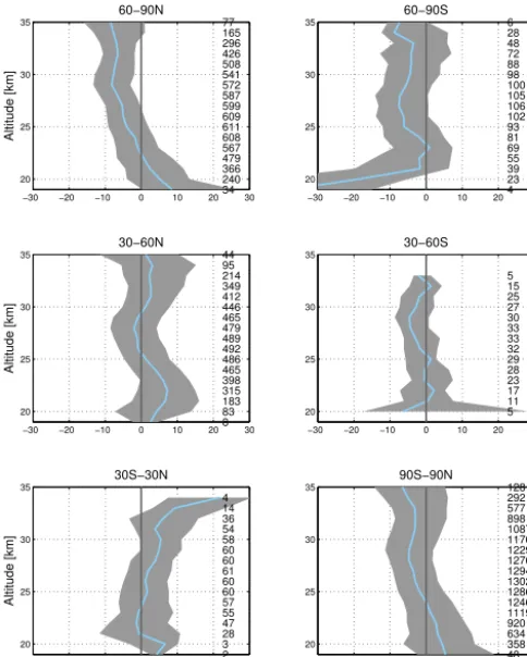
Figure 7. Interquartile ranges (shaded areas) and medians (solid lines) of the individual relative differences of GBL ozone profiles against NDACC ozonesondes for different latitude zones. The num-bers are the amount of co-located points at each altitude.
1. always remove the lowest retrieved point; 2. remove points with the reducedχ2>10;
3. remove points below 35 km where the relative error O3(error)
O3(density)>0.1, where O3(error)is the error estimate
of the retrieved density.
On average, theχ2screening removes∼0.3 points per pro-file and the error screening removes∼1.3 of the remaining points per profile. This kind of screening significantly im-proves the agreement in the 20–25 km range against all stud-ied reference data.
3.2 Results
Figure 7 shows the result against NDACC ozonesondes for the six latitude zones. Shown are interquartile ranges and medians of the differences. The numbers represent the num-bers of co-located pairs at each altitude. In these comparisons the median difference is always less than 10 % except lati-tudes 60–90◦S where the negative bias is more than−20 % at 19 km.
−20 −10 0 10 20 30 40 50
20 25 30 35 40 45 50 55 Difference [%] Altitude [km] 40−45 45−50 50−55 55−60 60−65 65−70 70−75 75−80 80−85 85−90
Figure 8. Median relative differences of GBL ozone profiles against GOMOS nighttime occultations for different solar zenith angles.
Figure 8 shows the comparison against GOMOS night oc-cultations for different solar zenith angles. There is a clear positive bias at around 50 km when the solar zenith angle is 75◦or larger. With smaller solar zenith angles the differences are rather similar. The large solar zenith angle observations account for 16 % of the GBL data and the GOMOS measure-ment geometry is such that these observations appear mostly at mid and high latitudes. We suspect that the 50 km bias is linked to stray light and its removal. GOMOS daytime data suffer from serious stray light contamination and in partic-ular the upper altitudes are sensitive to the accuracy of the removal method. We also note that the solar zenith angle seems to be the only parameter that clearly correlates with the 50 km bias. Some good individual profiles can be found even for high solar zenith angles but there is no clear pattern, or too few profiles to draw conclusions. Because the majority of the GBL measurements with a large solar zenith angle are distinctly biased at 50 km, in the remaining comparisons we only used the GBL data with the solar zenith angle smaller than 75◦.
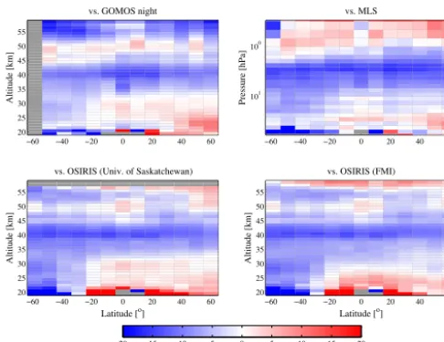
−60 −40 −20 0 20 40 60 20
25 30 35 40 45 50 55
Altitude [km]
vs. GOMOS night
−60 −40 −20 0 20 40 60
100
101
Pressure [hPa]
vs. MLS
−60 −40 −20 0 20 40 60
20 25 30 35 40 45 50 55
Latitude [o]
Altitude [km]
vs. OSIRIS (Univ. of Saskatchewan)
−60 −40 −20 0 20 40 60
20 25 30 35 40 45 50 55
Latitude [o]
Altitude [km]
vs. OSIRIS (FMI)
Difference [%]
−20 −15 −10 −5 0 5 10 15 20
Figure 9. Median relative differences of GBL ozone profiles against GOMOS nighttime occultations (upper left), MLS (upper right), OSIRIS University of Saskatoon version (lower left), and OSIRIS FMI version (lower right).
tropic/sub-tropic regions below 21 km but the deviations are large too. Remaining differences are below 10 % (and often
<5 %).
4 Discussion and summary
We have processed and released a GOMOS bright limb ozone data set. This data set roughly doubles the number of useful GOMOS ozone profiles. In general, the bias in the GBL ozone is less than 10 %, and often less than 5 %, but there is a clear 10–13 % negative bias at 40 km. The reason for this bias is uncertain but the most likely cause is the stray light contamination in the 300–320 nm band already noted by Tukiainen et al. (2011). Above the 45 km tangent height, we use UV wavelengths to retrieve ozone and below 40 km we use visible wavelengths. The retrieval method is sensitive to the transition from UV to visible and it is easily disturbed by stray light. As explained above, we scale the amount of stray light to get a smooth ozone profile in the 40 km transi-tion. This ad hoc approach works reasonably well in practice but better ways to switch between the different wavelength domains should be investigated in future.
The diurnal variation explains about 1–3 % of the observed 40 km bias as the GOMOS day measurements are made dur-ing the minimum of the diurnal cycle. At the 50 km altitude we have up to 50 % positive bias depending on the solar zenith angle. This bias cannot be explained by natural vari-ation; it indicates some problem in the retrieval, most likely related to the stray light and its correction. Until this issue is solved, it is recommended to only use GBL measurements with a solar zenith angle of less than 75◦ when using data from the altitudes above 45 km.
Table 4. Login information for accessing the GBL data.
Server ftp.fmi.fi
Login gomosGBL
Password kOs20mos!
In this work, we showed the accuracy of the GBL data as a function of latitude, altitude, and solar zenith angle (Figs. 7– 9). These are the most important variables affecting the over-all quality of the profiles. Beside these variables, we have also studied the effect of season, scattering angle, azimuth angle, albedo, and time, but they do not seem to correlate substantially with the bias. The quality of the GBL data could be summarized as follows. The accuracy of the GBL data is better than 10 % between 20 and 35 km. There is a negative bias at 35–45 km that has a consistent shape with all stud-ied observation conditions. Because of the regular shape, this bias is straightforward to correct if the data is used, for exam-ple, in time series studies. Above 45 km, the data is valid with the solar zenith angles of less that 75◦when the accuracy is approximately 15 % or better.
The GBL Level 2 files are available from the FMI’s FTP server and the login information is shown in Table 4. The file format is HDF5 (one file for each profile) and the total size of the whole data set is about 22 GB.
Acknowledgements. This study was funded by the European Space
Agency through the SPIN project (http://esa-spin.org) and by the Academy of Finland through the MIDAT project. The authors wish to thank the three referees for reviewing the manuscript and for suggesting relevant corrections. The authors also appreciate the MLS and OSIRIS teams for sharing their data. Special thanks go to Viktoria Sofieva for valuable suggestions. The (ozone sounding) data used in this publication were obtained as part of the Network for the Detection of Atmospheric Composition Change (NDACC) and are publicly available (see http://www.ndacc.org).
Edited by: C. von Savigny
References
Adams, C., Strong, K., Batchelor, R. L., Bernath, P. F., Brohede, S., Boone, C., Degenstein, D., Daffer, W. H., Drummond, J. R., Fogal, P. F., Farahani, E., Fayt, C., Fraser, A., Goutail, F., Hen-drick, F., Kolonjari, F., Lindenmaier, R., Manney, G., McElroy, C. T., McLinden, C. A., Mendonca, J., Park, J.-H., Pavlovic, B., Pazmino, A., Roth, C., Savastiouk, V., Walker, K. A., Weaver, D., and Zhao, X.: Validation of ACE and OSIRIS ozone and NO2 measurements using ground-based instruments at 80◦N, Atmos. Meas. Tech., 5, 927–953, doi:10.5194/amt-5-927-2012, 2012. Adams, C., Bourassa, A. E., Bathgate, A. F., McLinden, C. A.,
II dataset, Atmos. Meas. Tech., 6, 1447–1459, doi:10.5194/amt-6-1447-2013, 2013.
Bertaux, J. L., Kyrölä, E., Fussen, D., Hauchecorne, A., Dalaudier, F., Sofieva, V., Tamminen, J., Vanhellemont, F., Fanton d’Andon, O., Barrot, G., Mangin, A., Blanot, L., Lebrun, J. C., Pérot, K., Fehr, T., Saavedra, L., Leppelmeier, G. W., and Fraisse, R.: Global ozone monitoring by occultation of stars: an overview of GOMOS measurements on ENVISAT, Atmos. Chem. Phys., 10, 12091–12148, doi:10.5194/acp-10-12091-2010, 2010.
Degenstein, D. A., Bourassa, A. E., Roth, C. Z., and Llewellyn, E. J.: Limb scatter ozone retrieval from 10 to 60 km using a multiplicative algebraic reconstruction technique, Atmos. Chem. Phys., 9, 6521–6529, doi:10.5194/acp-9-6521-2009, 2009. ESA: GOMOS Level 2 Product Quality Readme File, available
at: https://earth.esa.int/documents/700255/708000/RMF_0117_ GOM_NL%2P_Disclaimers.pdf (last access: 21 April 2015), 2012.
Froidevaux, L., Jiang, Y. B., Lambert, A., Livesey, N. J., Read, W. G., Waters, J. W., Browell, E. V., Hair, J. W., Avery, M. A., McGee, T. J., Twigg, L. W., Sumnicht, . G. K., Jucks, K. W., Margitan, J. J., Sen, B., Stachnik, R. A., Toon, G. C., Bernath, P. F., Boone, C. D., Walker, K. A., Filipiak, M. J., Harwood, R. S., Fuller, R. A., Manñey, G. L., Schwartz, M. J., Daffer, W. H., Drouin, B. J., Cofield, R. E., Cuddy, D. T., Jarnot, R. F., Knosp, B. W., Perun, V. S., Snyder, W. V., Stek, P. C., Thurstans, R. P., and Wagner, P. A.: Validation of Aura Microwave Limb Sounder stratospheric ozone measurements, J. Geophys. Res.-Atmos., 113, D15S20, doi:10.1029/2007JD008771, 2008. Kyrölä, E., Laine, M., Sofieva, V., Tamminen, J., Päivärinta, S.-M.,
Tukiainen, S., Zawodny, J., and Thomason, L.: Combined SAGE II-GOMOS ozone profile data set for 1984–2011 and trend anal-ysis of the vertical distribution of ozone, Atmos. Chem. Phys., 13, 10645–10658, doi:10.5194/acp-13-10645-2013, 2013. Livesey, N. J., Read, W. G., Froidevaux, L., Lambert, A.,
Man-ney, G. L., Pumphrey, H. C., Santee, M. L., Schwartz, M. J., Wang, S., Cofield, R. E., Cuddy, D. T., Fuller, R. A., Jarnot, R. F., Jiang, J. H., Knosp, B. W., Stek, P. C., Wagner, P. A., and Wu, D. L.: EOS MLS Version 3.3 Level 2 data quality and description document, JPL D-33509, Jet Propulsion Labora-tory, Version 3.3x-1.0, available at: https://mls.jpl.nasa.gov/data/ v3-3_data_quality_document.pdf (last access: 5 August 2015), 18 January 2011.
Llewellyn, E. J., Lloyd, N. D., Degenstein, D. A., Gattinger, R. L., Petelina, S. V., Bourassa, A. E., Wiensz, J. T., Ivanov, E. V., McDade, I. C., Solheim, B. H., McConnell, J. C., Haley, C. S., von Savigny, C., Sioris, C. E., McLinden, C. A., Griffioen, E., Kaminski, J., Evans, W. F., Puckrin, E., Strong, K., Wehrle, V., Hum, R. H., Kendall, D. J., Matsushita, J., Murtagh, D. P., Brohede, S., Stegman, J., Witt, G., Barnes, G., Payne, W. F., Piché, L., Smith, K., Warshaw, G., Deslauniers, D. L., Marc-hand, P., Richardson, E. H., King, R. A., Wevers, I., McCreath, W., Kyrölä, E., Oikarinen, L., Leppelmeier, G. W., Auvinen, H., Mégie, G., Hauchecorne, A., Lefèvre, F., de La Nöe, J., Ricaud, P., Frisk, U., Sjoberg, F., von Schéele, F., and Nordh, L.: The OSIRIS instrument on the Odin spacecraft, Can. J. Phys., 82, 411–422, doi:10.1139/p04-005, 2004.
McLinden, C. A., Bourassa, A. E., Brohede, S., Cooper, M., De-genstein, D. A., Evans, W. J. F., Gattinger, R. L., Haley, C. S., Llewellyn, E. J., Lloyd, N. D., Loewen, P., Martin, R. V.,
Mc-Connell, J. C., McDade, I. C., Murtagh, D., Rieger, L., von Savi-gny, C., Sheese, P. E., Sioris, C. E., Solheim, B., and Strong, K.: OSIRIS: A Decade of Scattered Light, B. Am. Meteorol. Soc., 93, 1845–1863, doi:10.1175/BAMS-D-11-00135.1, 2012. Meijer, Y. J., Swart, D. P. J., Allaart, M., Andersen, S. B., Bodeker,
G., Boyd, I., Braathen, G., Calisesi, Y., Claude, H., Dorokhov, V., von der Gathen, P., Gil, M., Godin-Beekmann, S., Goutail, F., Hansen, G., Karpetchko, A., Keckhut, P., Kelder, H. M., Koele-meijer, R., Kois, B., Koopman, R. M., Kopp, G., Lambert, J.-C., Leblanc, T., McDermid, I. S., Pal, S., Schets, H., Stubi, R., Suortti, T., Visconti, G., and Yela, M.: Pole-to-pole validation of Envisat GOMOS ozone profiles using data from ground-based and balloon sonde measurements, J. Geophys. Res.-Atmos., 109, D23305, doi:10.1029/2004JD004834, 2004.
Sakazaki, T., Fujiwara, M., Mitsuda, C., Imai, K., Manago, N., Naito, Y., Nakamura, T., Akiyoshi, H., Kinnison, D., Sano, T., Suzuki, M., and Shiotani, M.: Diurnal ozone variations in the stratosphere revealed in observations from the Superconduct-ing Submillimeter-Wave Limb-Emission Sounder (SMILES) on board the International Space Station (ISS), J. Geophys. Res.-Atmos., 118, 2991–3006, doi:10.1002/jgrd.50220, 2013. Taha, G., Jaross, G., Fussen, D., Vanhellemont, F., Kyrölä, E., and
McPeters, R. D.: Ozone profile retrieval from GOMOS limb scat-tering measurements, J. Geophys. Res.-Atmos., 113, D23307, doi:10.1029/2007JD009409, 2008.
Tamminen, J., Kyrölä, E., Sofieva, V. F., Laine, M., Bertaux, J.-L., Hauchecorne, A., Dalaudier, F., Fussen, D., Vanhellemont, F., Fanton-d’Andon, O., Barrot, G., Mangin, A., Guirlet, M., Blanot, L., Fehr, T., Saavedra de Miguel, L., and Fraisse, R.: GOMOS data characterisation and error estimation, Atmos. Chem. Phys., 10, 9505–9519, doi:10.5194/acp-10-9505-2010, 2010.
Tukiainen, S., Hassinen, S., Seppälä, A., Auvinen, H., Kyrölä, E., Tamminen, J., Haley, C. S., Lloyd, N., and Verronen, P. T.: Description and validation of a limb scatter retrieval method for Odin/OSIRIS, J. Geophys.l Res.-Atmos., 113, D04308, doi:10.1029/2007JD008591, 2008.
Tukiainen, S., Kyrölä, E., Verronen, P. T., Fussen, D., Blanot, L., Barrot, G., Hauchecorne, A., and Lloyd, N.: Retrieval of ozone profiles from GOMOS limb scattered measurements, Atmos. Meas. Tech., 4, 659–667, doi:10.5194/amt-4-659-2011, 2011. van Gijsel, J. A. E., Swart, D. P. J., Baray, J.-L., Bencherif, H.,
Claude, H., Fehr, T., Godin-Beekmann, S., Hansen, G. H., Keck-hut, P., Leblanc, T., McDermid, I. S., Meijer, Y. J., Nakane, H., Quel, E. J., Stebel, K., Steinbrecht, W., Strawbridge, K. B., Tatarov, B. I., and Wolfram, E. A.: GOMOS ozone pro-file validation using ground-based and balloon sonde measure-ments, Atmos. Chem. Phys., 10, 10473–10488, doi:10.5194/acp-10-10473-2010, 2010.
Verronen, P. T., Kyrölä, E., Tamminen, J., Sofieva, V. F., Clar-mann, T., Stiller, G. P., KaufClar-mann, M., Lopez-Puertas, M., Funke, B., and Bermejo-Pantaleon, D.: A Comparison of Daytime and Night-Time Ozone Profiles from GOMOS and MIPAS, in: Proceedings of the Envisat Symposium 2007, Montreux, Switzerland, ESA SP-636, July 2007, 462479, available at: https://earth.esa.int/workshops/envisatsymposium/ proceedings/sessions/2A3/462479bv.pdf (last access: 5 August 2015), 2007.