www.ocean-sci.net/7/445/2011/ doi:10.5194/os-7-445-2011
© Author(s) 2011. CC Attribution 3.0 License.
Ocean Science
An ECOOP web portal for visualising and comparing distributed
coastal oceanography model and in situ data
A. L. Gemmell1, R. M. Barciela2, J. D. Blower1, K. Haines1, Q. Harpham3, K. Millard3, M. R. Price2, and A. Saulter2 1Environmental Systems Science Centre, Harry Pitt Building, 3 Earley Gate, Whiteknights, University of Reading,
Reading, RG6 6AL, UK
2The Met Office, Fitzroy Road, Exeter, Devon, EX1 3PB, UK
3HR Wallingford, Howbery Park, Wallingford, Oxfordshire, OX10 8BA, UK Received: 31 December 2010 – Published in Ocean Sci. Discuss.: 28 January 2011 Revised: 17 May 2011 – Accepted: 17 June 2011 – Published: 4 July 2011
Abstract. As part of a large European coastal operational oceanography project (ECOOP), we have developed a web portal for the display and comparison of model and in situ marine data. The distributed model and in situ datasets are accessed via an Open Geospatial Consortium Web Map Ser-vice (WMS) and Web Feature SerSer-vice (WFS) respectively. These services were developed independently and readily in-tegrated for the purposes of the ECOOP project, illustrating the ease of interoperability resulting from adherence to inter-national standards.
The key feature of the portal is the ability to display co-plotted timeseries of the in situ and model data and the quan-tification of misfits between the two. By using standards-based web technology we allow the user to quickly and easily explore over twenty model data feeds and compare these with dozens of in situ data feeds without being concerned with the low level details of differing file formats or the physical lo-cation of the data.
Scientific and operational benefits to this work include model validation, quality control of observations, data assim-ilation and decision support in near real time. In these areas it is essential to be able to bring different data streams together from often disparate locations.
1 Introduction
Marine scientists use highly diverse sources of data, includ-ing in situ measurements, remotely-sensed information and the results of numerical simulations. The ability to access, visualize, combine and compare these datasets is at the core
Correspondence to: A. L. Gemmell ([email protected])
of scientific investigation, but such tasks have hitherto been hindered by a fundamental lack of harmonization across data products and the lack of fast efficient online tools to exploit marine datasets available through the internet. As a result, much valuable data remains underused. As models become larger and increasingly complex, and sources of observed data become more numerous, it is important to be able to ac-cess and compare this growing amount of data efficiently, to ensure cross-checking and consistency between models and observations.
standard for storing such dense multi-dimensional data, along with the Climate and Forecast (CF) metadata con-vention for describing the content of NetCDF files in their file headers (Blower et al., 2009a). There is much cur-rent research interest in bringing together the worlds of GIS and 4-D environmental data to develop “4-D GIS” sys-tems. Groups have therefore developed OGC-based sys-tems for encoding environmental data (e.g. CSML – Cli-mate Science Modelling Language, Woolf et al., 2006; Marine Markup Language, http://www.ercim.eu/publication/ Ercim News/enw57/matthews.html), serving data (e.g. Best et al., 2007; de La Beaujardiere, 2009) and visualizing data (e.g. Blower et al., 2009b; Wei et al., 2009; Huang, 2003).
The Godiva2 project (Blower et al., 2009b) provides the starting point for the work presented here. It provides an efficient means of exploring 4-D environmental model data by generating 2-D maps or 3-D map-movies from data in CF-NetCDF files for remote viewing on an interactive inter-face based upon OpenLayers, an open-source browser-based map visualization library. The project uses the ncWMS soft-ware (http://ncwms.sf.net/) which generates 2-D maps fast enough for use in real-time interactive data browsing of large datasets. This software has been widely adopted by research institutes, government agencies and private industry for pre-senting operational marine forecasts (e.g. at the UK Met Of-fice) and satellite imagery (e.g. NEODAAS, Plymouth Ma-rine Laboratory). The software has also been adopted as the basis of the viewing interface for the GMES Marine Core Services project MyOcean (http://www.myocean.eu).
The aim of the European COastal sea Operational Observ-ing and forecastObserv-ing system Project (ECOOP, www.ecoop.eu) was to “build up a sustainable pan-European capacity in providing timely, quality assured marine services (includ-ing data, information products, knowledge and scientific ad-vices) in European coastal-shelf seas”. A key requirement was to develop a web portal that visualises and compares physical and biological marine data from both numerical models and in situ observations. We discuss the technical choices for viewing and interacting with the in situ data and relating it to the gridded model data. We also showcase the achievements of the ECOOP portal in its final form and go on to discuss the lessons learned and the further developments required in order to improve the system for future scientific applications requiring the viewing of combined model and observational datasets.
Section 2 discusses the datasets available through the ECOOP project as examples of the challenges required to be overcome. Section 3 first discusses the technical options for incorporating point data into the Godiva2 map viewing tool. We then discuss the architecture chosen and finally the scope of the ECOOP portal that was operational at the end of the project. Section 4 discusses some of the scientific uses this portal has been put to and Sect. 5 provides further discussion and conclusions particularly on the strengths and weaknesses of the current system and the plans for future developments.
2 Marine dataset distribution within Europe
2.1 Model forecast data
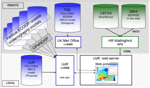
Many groups in Europe are now involved in operational ocean modelling and are able to provide daily or weekly fore-casts of marine conditions in local European coastal sea ar-eas. The ECOOP project provided 23 different model data feeds to the web portal from 14 different ECOOP partners. In order to view all these data in a single web portal the model data need to be rendered into map images. These im-ages could be rendered at each data provider using a Web Map Service such as ncWMS (a federated approach), or they could be rendered at the central server at the Univer-sity of Reading (a centralized approach), with the data be-ing accessed from the data providers via the OPeNDAP pro-tocol. The use of OPeNDAP to serve data was mandatory in the project and so the easiest solution from the point of view of the data providers was the centralized approach, with most data feeds being sent to a single WMS for rendering into images. However, two partners (UK Met Office and Plymouth Marine Laboratory) were able to run their own ncWMS servers and therefore provide imagery directly to the web portal. In future the federated approach is preferred, as this avoids a data bottleneck at the central server; this ap-proach will be taken in the MyOcean project. The latest version of THREDDS (v4.2) includes an OPeNDAP service together with an embedded ncWMS service, therefore data providers will in future be able to provide both types of ser-vice using the same software. The complete list of model forecast providers can be found in Table 1 and Fig. 1 shows the data regions of model output provided. Note that there is a very low barrier to entry for the serving of additional CF-compliant model data using our system. If the data providers provide data through an OPeNDAP server, then it is a trivial matter to incorporate these new data feeds into the portal. 2.2 In situ observational data
Table 1. Full list of ECOOP partner institutes providing model data to the portal. Numbers match with model areas shown in Fig. 1.
Institute Country
1. Bundesamt f¨ur Seeschifffahrt und Hydrographie (BSH) Germany 2. Danish Meteorological Institute (DMI) Denmark
3. Mercator France
4. Previmer France
5. Maretec Portugal
6. The Marine Institute Ireland
7. UK Meteorological Office (UKMO) UK
8. Plymouth Marine Laboratory (PML) UK
9. Istituto Nazionale di Geofisica e Vulcanologia (INGV) Italy
10. University of Athens Greece
11. Institute of Oceanology (IO-BAS) Bulgaria 12. National Institute for Marine Research and Development (NIMRD) Romania 13. Marine Hydrophysical Institute (MHI) Ukraine 14. Mediterranean Institute for Advanced Studies (IMEDEA) Spain
Fig. 1. The model regions available in the portal. Numbers
repre-sent the institutes serving the model data as per Table 1.
SEPRISE data only contain physical ocean variables such as temperature, salinity and current data. CEFAS (Centre for the Environment, Fisheries and Aquaculture Science), col-lect data from around the UK coasts using “SmartBuoys” which monitor both physical and biogeochemical variables which are of interest for an increasing number of applica-tions. These SmartBuoy data were also obtained daily by HR Wallingford and served to the ECOOP portal via WFS in the same uniform CSML format as the SEPRISE data. The full range of model and in situ data which may be compared using the portal is given in Table 2.
3 Technical approach
The architecture of the system is illustrated in Fig. 2. The ncWMS software has been described elsewhere (Blower et al., 2009b) therefore in the following sections we focus on
Fig. 2. Architecture of the system. Model data (blue) are ingested
into the portal via an instance of ncWMS at the University of Read-ing (UoR), and an instance of ncWMS at the UK Met Office. in situ data (green) are ingested into the portal via the WFS at HR Wallingford serving CSML XML.
the other elements of the system – the use of WFS for serving in situ data (Sect. 3.1) and the web portal itself (Sect. 3.2).
The WFS for serving the portal with in situ point data, and the WMS for serving the portal with gridded model data were developed independently, and only integrated later for the purposes of the work presented here. This modular ap-proach increased flexibility and allowed both sides of the sys-tem to be developed and upgraded independently. Integration of the two data streams at the portal was facilitated by sup-port for WMS layers and point features in the OpenLayers library (see Sect. 3.2).
3.1 Standards-based serving of in situ data
Table 2. Model data types and their corresponding in situ data types, sources, and nature of comparison. Where the comparison is given as
qualitative this indicates that a dual axis plot of both data are shown, and qualitative correlations can be expected.
Model data type in situ data type in situ data source Comparison
Sea water temperature (Celsius) Sea water temperature (Celsius) SEPRISE, SmartBuoys Exact match
Sea water salinity (P.S.U) Sea water salinity (P.S.U) SEPRISE, SmartBuoys Exact match
Sea water velocity (m s−1) Sea water velocity (m s−1) SEPRISE Exact match Chlorophyll-a(mg m−3) Fluorescence (Arbitrary Unit) SmartBuoys Qualitative Dissolved Oxygen
Conc. (m mol m−3)
Oxygen saturation (%) SmartBuoys (Liverpool Bay, Warp Estuary only)
Converted according to Weiss (1970)
Photosynthetically active radiation (W m−2)
Irradiance (E×10−6m2s−1) SmartBuoys Qualitative
Suspended particulate matter (35 µ) (kg m−3)
Turbidity (F.T.U.) SmartBuoys Qualitative
Suspended particulate matter (2 µ) (kg m−3)
Turbidity (F.T.U.) SmartBuoys Qualitative
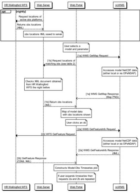
into the portal owing to its adherence to recognised interna-tional standards, complementing the existing OGC Web Map Service used for the model data, and increasing the reusabil-ity of existing code and tools. The OGC WFS standard speci-fies that data should be encoded as XML adhering to a GML application schema. For this we chose to use CSML, and in particular the PointSeries FeatureType. CSML is specif-ically tailored to represent features of relevance to the cli-mate sciences and comprises 13 FeatureTypes, of which the PointSeriesFeature represents a timeseries at a fixed location. There are two different queries which are made in order to retrieve the in situ data. The first step is a query to determine which of the geographically static in situ stations were actively measuring data for the dates and parameter of interest. The response is a set of locations of in situ stations. When one of these stations is interrogated the second query is to request the data from that station for a period of time. These two queries both correspond to GetFeature requests within the OGC WFS standard. In the case of the first query an example query string (minus this initial server URL and port number) is:
wfs?request=GetFeature&service=WFS&version=1.1.0&
typeName=hrw:ECOOPTimeSeries.
In the case of the second query an example query string (minus the initial server URL and port number) is:
wfs?request=GetFeature&service=WFS&version=1.1.0& typeName=ldip:ECOOPSmartBuoyTimeSeries&filter=FILTER
where “FILTER” is a placeholder for an XML string to filter the results which adheres to the OGC Filter Encoding Im-plementation specification (http://www.opengeospatial.org/ standards/filter). For example, the filter is often used to select only a single FeatureType based on its ID and the parameter being measured. In this case, the required start and end times of the in situ data were also used in the filter.
However, here we are extending the WFS specification somewhat. The logical Features in question are CSML PointSeries features. Each Feature is an entire timeseries, which may be very long. For our application, we need to access subsets of these features, which are themselves PointSeriesFeatures. There is no support in version 1 of the WFS standard for subsetting a feature (features must be served whole), and hence our WFS implementation (GeoServer) was not able to support this requirement in a straightforward manner. The system was therefore designed so that each individual measurement in each timeseries was stored as a point measurement in the database that sits be-hind the WFS. The request for a particular time range leads to the extraction of a number of these individual point fea-tures, which are produced by GeoServer as a single XML document. This document (containing several point features) is then transformed by an XSLT transformation into a CSML document which contains a single PointSeriesFeature. The net effect is that the user of the WFS can request subsets of logical PointSeriesFeatures; this extends the standard but was necessary to fulfil the requirements of the project. We discuss in Sect. 5 below possible alternatives to this architec-ture.
HR Wallingford WFS
HR Wallingford WFS
Web Server
Web Server
Web Portal
Web Portal
ncWMS
ncWMS Request locations of
active obs platforms Returns obs locations (XML)
obs locations XML saved to server opt [nightly]
User selects a model and parameter
[1a] WMS GetMap Request [1b] Request locations of
matching obs (see table 2)
Accesses model NetCDF data (either local or via OPeNDAP)
Checks XML document obtained from HR Wallingford WFS the night before
[1a] WMS GetMap Response (Map PNG) [1b] Return obs locations
(XML)
Map of model data with obs locations shown
User clicks an ob
[2a] WMS GetFeatureInfo Request [2b] WFS GetFeature Request
Accesses model NetCDF data (either local or via OPeNDAP)
[2a] WMS GetFeatureInfo Response (XML) [2b] GetFeature Response
(CSML XML)
Constructs Model-Obs Timeseries plot
If user expands timeseries then requests 2a and 2b are repeated
Fig. 3. Sequence diagram showing the calls made from the Godiva2
web portal (running in the browser client) to request the model and obs data, as well as the responses returned.
determine what data are present for the dates and parameter of interest being currently displayed as a model field in the ECOOP portal. It was important to make the process of re-turning the positions of the available in situ data as efficient as possible to avoid a prolonged wait before the locations of the platforms can be displayed in the portal. However, it was taking several minutes for the WFS to filter the more than 800 FeatureTypes being served to return the locations of relevant data. This bottleneck was eventually avoided because the in situ data are only updated once per day so it was possible to query the WFS server each night and save the resulting XML document of CSML FeatureTypes locally. This caching re-duces the time to query the data from several minutes to sec-onds. Work is ongoing to increase the WFS efficiency (see Sect. 5) and preliminary results indicate that server caching of data will no longer be necessary in the next generation of the HR Wallingford WFS.
In Fig. 3 the request 2b is only enacted when the client clicks on one of the in situ data icons on the portal, at which point that actual in situ data item is retrieved for display. The result of such a query is a CSML document, e.g. Fig. 4 rep-resenting sea water temperature data from the Liverpool Bay
Fig. 4. Example of CSML XML returned from the WFS,
represent-ing sea water temperature data from the Liverpool Bay SmartBuoy. Note that the 10-day list of times and values as been truncated for brevity.
SmartBuoy. Note that the 10-day list of times and values has been truncated for brevity.
3.2 The web portal
It can be seen from Fig. 3 that the web portal coordinates the delivery and integration of data from the various sources. The web portal runs entirely in the browser client (http: //www.resc.reading.ac.uk/ecoop obs portal) and its primary roles are to (a) respond to the user’s requests and to del-egate these requests to the relevant actor and (b) receive the respective responses and present these to the user in-cluding combining of multiple responses where appropri-ate. The portal employs two Javascript libraries in order to fulfil these roles – OpenLayers (openlayers.org) and Flot (http://code.google.com/p/flot).
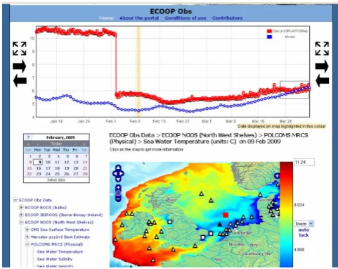
Fig. 5. Portal screenshot showing an extended timeseries of sea
water temperature (red line, two-hourly data feed) from the K13 Platform in the North Sea (solid black triangle) and from the POL-COMS MRCS model (blue line, daily average). The elevated tem-peratures present in the observed data for the first third of the time-series are erroneous, and the correction of this problem is clearly seen as later temperatures are in much closer agreement with the model data. The black rectangle on the right of the timeseries plot denotes the area of the zoomed-in timeseries in Fig. 7, which also contains a timeseries from the OysterGround SmartBuoy to the North East of the K13 platform (red square).
cluster strategy or to render the observed locations onto an image overlay.
When in situ data are requested they are displayed above the map in a timeseries, along with an equivalent timeseries sampled from the model data being concurrently displayed. These timeseries plots, which can be seen in Figs. 5–8, are produced by the Flot graphing library. This graph can be zoomed for more detail in a particular region, and the user can mouse-over the data points to reveal their precise time and value. The start and end of the timeseries can be in-crementally expanded or contracted. Each time this happens the data are cached, meaning that the timeseries can be con-tracted and expanded again without unnecessary calls to the server. Figure 5 illustrates a view of the portal after requests 1a, 1b, 2a, and 2b have been successfully executed. In ad-dition, the default timeseries of 10 days has been expanded a number of times. One benefit of using a dynamic plot-ting library as opposed to static plots is the ability to correct on-the-fly for rogue values that distort the y-axis scaling as illustrated in Fig. 6.
4 Scientific and operational applications
There are many benefits that may be derived from the ability to quickly and easily compare model and in situ data over
Fig. 6. Sea water temperature (◦C) from the AberporthBuoy plat-form. One of the benefits of using a dynamic plotting library in the web portal is that if rogue data points are disturbing the y-axis scal-ing, they may be highlighted (top panel) and removed, resulting in auto-scaling of the y-axis to the correct range for the genuine data values (bottom panel).
the web. Calibrating observations against model background data in order to detect biases and other gross errors is one application. Once the observations are calibrated they can be used for testing the detailed accuracy of the numerical mod-els. The best analysis should come from combining model and observations in a data assimilation process and this can benefit greatly from displaying the results before and after as-similation along with either assimilated or independent data, or displaying the success of a forecast made using assimi-lated initial conditions. Decision support systems will benefit from the display of multiple model and data streams together to add confidence to the decision making process. In the fol-lowing sections we describe examples of the benefits which the current work brings to these areas.
4.1 Observational quality control
It is often assumed that in situ observations represent the “truth” to which model and remotely-sensed data should be compared in order to improve their accuracy. This is not the case, as in situ instruments are simply attempting to measure the true state of the system, and are subject to errors and bi-ases in doing so. One can consider two major categories of errors in in situ measurements:
1. Accuracy errors inherent in the instrument, e.g. a tide gauge may be capable of measuring sea surface height only to within 1 cm.
Type 1 errors sometimes appear as quantizations in time-series plots – the observed parameter only takes up certain values resolved by the instrument. Type 2 errors are often unexpected and may be identified through routine compar-isons with other data sources, such as model background data. Figure 5 shows one of the SEPRISE platforms initially displaying erroneous temperature data, which was noticed upon comparison with POLCOMS MRCS temperature fields in the portal, prior to 1 February 2009. The data acquisition and transfer process was checked by staff at SMHI who dis-covered the error and rectified the problem (the data feed had erroneously been coming from another buoy entirely) after 1 February. Viewed in isolation, prior to comparison with model data within the portal, the excessively high observed temperatures had not been noticed.
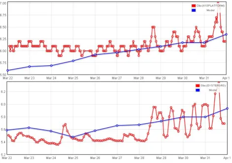
Figure 7 shows a zoom of the model data matchup for both the SEPRISE data in Fig. 5 (upper panel) and for the Smart-Buoy data about 100 km to the North East of the SEPRISE location in Fig. 5 (lower panel). The zoomed-in plot shows up diurnal and tidal timescales for the same period. It is no-ticeable that, particularly in the early phase of the timeseries, the SEPRISE data illustrate the quantization phenomenon described above, whereas the SmartBuoy data show a more reliable picture of diurnal variation in sea surface tempera-tures. It is clear from both timeseries that there is an increase in the diurnal and tidal signal during and after 28 March. In the case of the SEPRISE data this signal is dominated by an approximately 24 h cycle, with a weaker approximately 12 h cycle, whereas the two frequencies are more equally repre-sented in the SmartBuoy data. This type of matchup across instruments and nearby locations demonstrates how the abil-ity to cross reference observational and model datasets pro-vides interesting and useful calibration information.
4.2 Validation of ocean models
The ability to compare models with in situ observations is critical to the model validation and improvement process. The present work ensures that there is a low barrier to model validation against in situ observations by bringing the two datasets together in timeseries plots. In Fig. 5 during the ini-tial portion of the timeseries the model acts as a test for the observed data (Sect. 4.1), while during the later period, af-ter correction, the observed data acts as a test for the model data. One can see that there is overall agreement between ob-servation and model for this portion of the timeseries, with both datasets starting to show a slow warming into Spring. Although the model starts off too cold by about 1◦C, this
deficit disappears by the end of March. This model is not run with a diurnal cycle forcing and so we are unable to test the difference in diurnal behaviour noted in Fig. 7.
Another example of model validation is shown in Fig. 8 in which ocean velocity output from the University of Athens Aegean and Levantine Eddy Resolving MOdel (ALERMO, Korres and Lascaratos, 2003) is compared with current
Fig. 7. Zoomed in timesereies from Fig. 5 of sea water
tempera-ture (◦C) showing diurnal and tidal variation in the K13 observing platform and MRCS model (upper panel). Also comparing with the OysterGround SmartBuoy to the north east of the K13 platform (lower panel).
meter data from the E1M3ACRETANSEA in situ station. ALERMO has a horizontal resolution of 1/30◦×1/30◦ and a vertical resolution of 25 logarithmically distributed sigma levels. ALERMO is one-way coupled with the SKIRON weather forecasting system (Kallos, 1997) which provides air temperature and relative humidity at 2 m above the sea surface, wind velocity at 10 m, sea level atmospheric pres-sure, net shortwave radiation at the sea surface, downward longwave radiation and precipitation rate. Here we can see that the model daily average output for velocity is under-representing the daily mean velocities that we could infer from the in situ station. This is not entirely surprising given the model resolution and forcing used, but it does give an immediate quantitative evaluation of the model discrepan-cies. This example also illustrates a potential pitfall when comparing model and in situ velocities with differing time resolution. The model velocity is a daily mean, whereas the in situ velocities are instantaneous. If the latter were aver-aged to create a daily mean then this could be lower than a simple numerical average of the velocity magnitudes owing to potential changes in current direction.
4.3 Data assimilation systems
Fig. 8. Sea water velocity output from the ALERMO model from
the University of Athens compared to current meter data from the E1M3ACRETANSEA in situ station (black triangle).
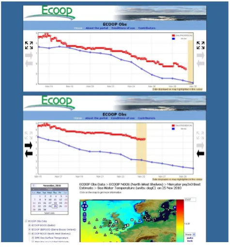
25 November utilising all the observations up till that date. The observations in this case are taken further forward un-til 2 December to show the level of agreement. Note that the SEPRISE buoy data being used here is independent and will not have been included in the assimilation procedure. It can be seen that although these buoy data have not been as-similated, the actual variations in SST through the period are better reproduced from the best estimate products. Compar-isons such as this shown in a screenshot from our web portal allow scientists and users to interpret and use the model fore-cast and analysis results much more easily without specialist knowledge of the data sets. They can compare for themselves the various models and forecasts with the in situ data both before and after data have been assimilated into the model output.
4.4 Decision support in near real time
Operational and pre-operational physical-biogeochemical models routinely generating ecological products now exist (Siddorn et al., 2007; Brasseur et al., 2009) and their prod-ucts, including forecasts, are being disseminated in near-real time to end-users (www.myocean.eu). The South West Algal Pilot Project (SWAPP) and its successor, the Al-gaRisk project (www.npm.ac.uk/rsg/projects/algarisk, Bar-ciela et al., 2009), assessed and demonstrated the feasibility of this approach for forecasting algal blooms affecting the coastal waters of the UK, through the combination of satel-lite observations, model and meteorological data (Mahdon et al., 2010). Other initiatives, such as the European Marine Strategy Framework Directive, are likely to benefit from in-corporating web technology, such as the web portal described
Fig. 9. Portal screenshot showing a timeseries of sea water
tempera-ture (red line, two-hourly data feed) from the Frederica platform off the East coast of Denmark (solid black triangle) and from the Mer-cator psy2v3 model (blue line, daily average). The lower timeseries is from 25 November, and the upper timeseries is from 30 Novem-ber. Note that the more recent timeseries represents a best estimate based on more available observed data which have been assimilated into the model, and hence shows a better fit with the Frederica in situ data feed.
here, as part of a wider set of monitoring tools required to es-tablish a successful environmental monitoring programme. It is important that these tools use standards to guarantee in-teroperability of different national components at larger pan-European scales..
5 Technical discussion
The comparison of in situ and model data from disparate sources is a common problem in the Earth and environmental sciences. This project has employed a number of tools and standards to address this problem. It is important to develop tools such as this in a manner consistent with international standards such as INSPIRE, and those of the OGC in order to facilitate greater interoperability and reusability. Neither the WFS standard, nor the CSML data format, are widely used in ocean science and there is little previous work in this area to guide the development of the portal described here. We therefore discuss WFS and CSML in this section, and compare them with other options for the serving of in situ data.
There is no support in version 1 of the WFS standard for subsetting a feature, and hence our method of returning a specific portion of a CSML PointSeriesFeature had to be achieved through serving features from the WFS which were single points in space and time, and then amalgamating these into the required portions of timeseries in the form of a late-stage transformation to a CSML PointSeries feature. This is not a very efficient method, but was chosen to allow the re-use of the GeoServer software with only relatively minor modifications.
Work is ongoing to increase the efficiency of serving data from the WFS by using a relational database to store the in situ data and by upgrading to the latest version of GeoServer. In addition, the final step in returning the in situ data to the user – conversion of the basic GML Point Features from the WFS into a CSML PointSeries Feature – is a known bottle-neck and may be omitted in future versions of the WFS. This will result in the quicker return of data to the user, whilst still maintaining standards-compliance. In this scenario there is a trade-off between increased efficiency and the loss of the more application domain tailored CSML PointSeries Fea-tures.
In contrast to WFS, the Sensor Observation Service, SOS, has explicit support for the time dimension, and allows for the request of observations from a specific instant, multiple instances or periods of time and we would now consider SOS to be a good alternative standard for serving in situ time-series data. (SOS was not published as a standard at the time the work described in this paper was started.) In addi-tion to the support for the time dimension, SOS also has ex-plicit support for the observed property being measured. The OGC Oceans Interoperability Experiment (OGC OIE, http: //www.opengeospatial.org/projects/initiatives/oceansie) rec-ommended the use of SOS over WFS for in situ marine data citing the above benefits, as well as others such as in-creased potential for interoperability and schema and func-tional maintenance.
The recently published OGC Web Feature Service 2.0 Interface Standard (http://portal.opengeospatial.org/files/ ?artifact id=39967) is distinct from the WFS version 1 in
a number of ways including richer queries and support for splitting features. This new iteration of the WFS standard may thus prove to be a strong contender for the type of work described here, and it will be interesting to monitor take-up in future projects.
The method of data encoding is somewhat orthogonal to that of the standard for serving the data, and in the present study the use of CSML was successful in meeting the needs of the project. It has the advantage of being semantically precise and tailored for the climate sciences. However, there are not yet many clients capable of correctly parsing CSML, and depending on the nature of the problem the users and their client software, there remains a place for looser formats such as CSV (Comma Separated Value) as recommended in the SeaDataNet (www.seadatanet.org) project. Note that for-mats such as CSV are semantically weaker than CSML, for example, there is no clean separation between the “domain” and “range” (i.e. the independent and dependent variables). It is a more free-form format that relies to some extent on human interpretation, although an advantage of CSV is that it is more easily ingested into common tools such as spread-sheets. CSML is more precise but, as an XML format, is relatively verbose and hence inefficient to parse in browsers. As a hierarchical format, it is harder to ingest into spread-sheets than column-based formats such as CSV.
An alternative format is ObsJSON (http://code.google. com/p/xenia/wiki/ObsJSON) which is more compact and ef-ficient format for communication between the web server and the browser. In practice however web portal developers have limited control over the service types and data formats used by data providers, and thus must accommodate them as ef-fectively as possible. We anticipate that more data will be made available in ObsJSON format through the IOOS initia-tive (http://www.ioos.gov/).
Finally, we note that the use of the WMS standard for comparing disparate data can provide a challenge in terms of the choice of colour scales when gridded data are com-ing from different providers. In the present work, all the model data accessible in the portal are viewed by the ncWMS software, which enables a choice of colour scales. In a scenario where data were also coming from other WMS implementations, careful consideration would have to be given to the choice of colour scale. One possible option in this case is to consider the use of Styled Layer Descrip-tors (http://www.opengeospatial.org/standards/sld) – another OGC standard.
based data serving, will become critical for monitoring the marine and wider environment and environmental change on a national and international basis into the future.
Acknowledgements. This project was supported through the EU
ECOOP project and the BERR Public Sector Research Exploitation Fund: Third Round Capacity Building Funding for the National Centre for Ocean Forecasting. We would like to thank Patrick Gorringe for his strong support and help to use the SEPRISE dataset, CEFAS for their cooperation in making the SmartBuoy data available for comparison, and the Plymouth Marine Laboratory for making Met Office model output available including biological parameters. We would also like to thank the two anonymous reviewers for their helpful feedback.
Edited by: G. Korotaev
References
Barciela, R., Mahdon, R., Miller, P., Orrell, R., and Shutler, J.: AlgaRisk 08. A operational tool for identifying and pre-dicting the movement of nuisance algal blooms, Innovation for efficiency science programme, Environment Agency, 32 pp., SC070082/SR1, 2009.
Best, B. D., Halpin, P. N., Fujioka, E., Read, A. J., Qian, S. S., Hazen, L. J., and Schick, R. S.: Geospatial web services within a scientific workflow: Predicting marine mammal habitats in a dynamic environment, Ecol. Inform., 2(3), 210–223, 2007. Blower, J. D., Blanc, F., Clancy, R., Cornillon, P., Donlon, C.,
Hacker, P., Haines, K., Hankin, S. C., Loubrieu, T., Pouliquen, S., Price, M., Pugh, T., and Srinavasan, A.: Serving GODAE data and products to the ocean community, Oceanography, 22(3), 70– 79, 2009a.
Blower, J. D., Haines, K., Santokhee, A., and Liu, C.: Godiva2: In-teractive visualization of environmental data on the web, Philos. T. Roy. Soc. A., 367, 1035–1039, 2009b.
Brasseur, P., Gruber, N., Barciela, R., Brander, K., Doron, M., El Moussaoui, A., Hobday, A. J., Huret, M., Kremeur, A., Lehodey, P., Matear, R., Moulin, C., Murtugudde, R., Senina, I., and Svendsen, E.: Integrating Biogeochemistry and Ecology Into Ocean Data Assimilation Systems, Oceanography, 22(3), 206– 215, 2009.
de La Beaujardiere, J.: Serving ocean model data on the cloud, OCEANS 2009, MTS/IEEE Biloxi – Marine Technology for Our Future: Global and Local Challenges, 1–10, 2009.
Gibin, M., Singleton, A., Milton, R., Mateos, P., and Longley, P.: An exploratory cartographic visualization of London through the Google Maps API, Applied Spatial Analysis and Policy, 1(2), 85–97, 2008.
Guney, C., Duman, M., Uylu, K., Avci, O., and Celik, R. N.: Mul-timedia supported GIS in the internet (Case study: two Ottoman fortresses and a cemetery on the Dardanelles), CIPA 2003 XIXth International Symposium, 30 September–4 October 2003, An-talya, Turkey, 2003.
Huang, B.: Web-based dynamic and interactive environmental vi-sualization, Comput. Environ. Urban, 27, 623 pp., 2003. Kallos, G.: The regional weather forecasting system SKIRON: an
overview. Proceedings of the symposium on regional weather prediction on parallel computer environments, University of Athens, 1997.
Korres, G. and Lascaratos, A.: A one-way nested eddy resolv-ing model of the Aegean and Levantine basins: implemen-tation and climatological runs, Ann. Geophys., 21, 205–220, doi:10.5194/angeo-21-205-2003, 2003.
Mahdon, R., Barciela, R., Edwards, K., Miller, P., Shutler, J., Roast, S., Jonas, P., Murdoch, N., and Wither, A.: Advances in Op-erational Ecosystem Modelling and the Prediction of Nuisance Algal Blooms at the UK Met Office, submitted the ICES Confer-ence Proceedings, 2010.
Peterson, M.: International Perspectives on Maps and the Internet: An Introduction, Geoinformation and Cartography Part A, 3–10, 2008.
Rahim, S. T., Zheng, K., Turay, S., and Pan, Y.: Capabilities of multimedia GIS, Chinese Geogr. Sci., 9(2), 159–165. 1999. Siddorn, J. R., Allen, J. I., Blackford, J. C., Gilbert, F. J., Holt, J.
T., Holt, M. W., Osborne, J. P., Proctor, R., and Mills, D. K.: Modelling the hydrodynamics and ecosystem of the North-West European continental shelf for operational oceanography, J. Ma-rine Syst., 65, 417–429. 2007.
Wei, Y., Santhana-Vannan, S., and Cook, R.: Discover, visualize, and deliver geospatial data through OGC standards-based We-bGIS system, 17th International conference on geoinformatics, 1–16, 2009.
Weiss, R. F.: The solubility of nitrogen, oxygen and argon in water and seawater, Deep-Sea Res., 17, 721–735, 1970.