www.nonlin-processes-geophys.net/17/201/2010/ © Author(s) 2010. This work is distributed under the Creative Commons Attribution 3.0 License.
Nonlinear Processes
in Geophysics
The effect of shear on the generation of gravity waves
M. Humi
Department of Mathematical Sciences, Worcester Polytechnic Institute, 100 Institute Road, Worcester, MA 01609, USA Received: 2 December 2009 – Revised: 23 March 2010 – Accepted: 25 March 2010 – Published: 12 April 2010
Abstract. Previous research regarding the solutions of Long’s equation always presumed that the flow far upstream is without shear. In this paper we derive the proper form of this equation when shear is present. We then apply a sequence of transformations to this equation which make it possible to linearize it while preserving its physical contents. We then derive conditions under which the solutions of this linear equation admit the existence (or creation) of gravity waves. We present also a solution of this model equation when the presence of shear in the overall flow is “small”.
1 Introduction
Long’s equation (Long, 1952, 1953, 1955, 1959) models the flow of stratified incompressible fluid in two dimensions over terrain. When the base state of the flow (that is the un-perturbed flow field far upstream) is without shear the nu-merical solutions (in the form of steady lee waves) of this equation over simple topography (i.e. one hill) were stud-ied by many authors (Drazin, 1961, 1967; Durran, 1992; Lily, 1979; Peltier and Clarke, 1983; Smith, 1980, 1989, Yih 1967, Davis 1999). The most common approximation in these studies was to set Brunt-V¨ais¨al¨a frequency to a constant or a step function over the computational domain. More-over the values of two physical parameters which appear in this equation were set to zero. (These parameters control the stratification and dispersive effects of the atmosphere – see Sect. 2.) In this (singular) limit the nonlinear terms and one of the leading second order derivatives in the equation drop out and the equation reduces to that of a linear har-monic oscillator over two dimensional domain. Careful stud-ies (Lily, 1979) showed that these approximations set strong limitations on the validity of the derived solutions (Peltier and Clarke, 1983). An extensive list of references appears in (Baines, 1995; Carmen, 2002; Yih, 1980).
Correspondence to: M. Humi
Long’s equation also provides the theoretical framework for the analysis of experimental data (Shutts, 1988, 1994; Vernin, 2007) under the assumption of shearless base flow. (An assumption which, in general, is not supported by the data; Humi, 2004b).
An analytic approach to the study of the solutions of this nonlinear equation was initiated recently by the current au-thor (Humi, 2004a, 2006, 2007). We showed that for a base flow without shear and under rather mild restrictions the nonlinear terms in the equation can be simplified. Us-ing phase averagUs-ing approximation we derived for self sim-ilar solutions of this equation a formula for the attenuation of the stream function perturbation with height. This result is generically related to the presence of the nonlinear terms in Long’s equation. New representations of this equation in terms of the atmospheric density and terrain following coor-dinates were derived in (Humi, 2007, 2009). Partial results on the impact that shear can have on the generation and am-plitude of gravity waves when the base flow consists of “pure shear” were investigated by us in (Humi, 2006).
The objective of this paper is to study the nature of the solutions to Long’s equation when some shear is present in the base flow. Using conditions which depend solely on the base flow and Brunt-V¨ais¨al¨a frequency we characterize the qualitative nature of the perturbations from the base flow and their amplitude with height. These results are independent of the actual detailed description of the terrain that caused these perturbations. Furthermore we derive conditions under which these perturbations are not oscillatory i.e. no gravity waves are generated by the flow. To our best knowledge this issue was never considered in the literature before (at least in the context of Long’s equation).
The plan of the paper is as follows: Sect. 2 presents the different forms of Long’s equation and the solution of its simplified version without shear. In Sect. 3 we derive the (analytic) solution of this simplified equation using terrain following formulation of Long’s equation in the presence of shear. Section 4 presents several transformations of Long’s equation which lead to it linearization while conserving its physical contents. We then solve this linearized equation when the mixture of shear in overall base flow is “small”. Section 5 presents constraints on the generation of gravity waves in the presence of shear using the linearized equation which was derived in Sect. 4. Setion 6 considers the case of base flow consisting of “pure shear”. We end up in Sect. 7 with summary and conclusions.
2 Long’s equation
2.1 Derivation of the equation
In two dimensions(x,z)the flow of a steady inviscid and in-compressible stratified fluid (in the Boussinesq approxima-tion) is modeled by the following equations:
ux+wz=0 (1)
uρx+wρz=0 (2)
ρ (uux+wuz)= −px (3)
ρ (uwx+wwz)= −pz−ρg (4)
where subscripts indicate differentiation with respect to the indicated variable, u=(u,w) is the fluid velocity, ρ is its densitypis the pressure andgis the acceleration of gravity. We can non-dimensionalize these equations by intro-ducing
¯ x = x
L, z¯= N0
U0
z, u¯= u U0
, w¯=LN0 U02 w ¯
ρ= ρ ρ0
, p¯= N0 gU0ρ0
p (5)
whereLrepresents a characteristic length, andU0,ρ0
repre-sent respectively the free stream velocity and density. N0is
the characteristic Brunt-Vaisala frequency N02= −g
ρ0
dρ0
dz. (6)
In these new variables Eqs. (1)–(4) take the following form (for brevity we drop the bars)
ux+wz=0 (7)
uρx+wρz=0 (8)
βρ(uux+wuz)= −pz (9)
βρ (uwx+wwz)= −µ−2(pz+ρ) (10)
where β=N0U0
g (11)
µ= U0 N0L
. (12)
βis the Boussinesq parameter (Baines, 1995; Carmen, 2002) which controls stratification effects (assumingU06=0) andµ
is the long wave parameter which controls dispersive effects (or the deviation from the hydrostatic approximation). In the limitµ=0 the hydrostatic approximation is fully satisfied (Baines, 1995; Carmen, 2002).
In view of Eq. (7) we can introduce a stream functionψ so that
u=ψz, w= −ψx. (13)
After a long (and intricate) algebra one can show that ρ=ρ(ψ )and derive the following equation forψ(Dubreil, 1934; Long, 1953, 1954)
ψzz+µ2ψxx−N2(ψ )
z+β 2
ψz2+µ2ψx2
=S(ψ ) (14) where
N2(ψ )= −ρψ
βρ (15)
is the nondimensional Brunt-Vaisala frequency andS(ψ )is some unknown function which can be determined by making proper assumptions on the upstream disturbance (see Baines, 1995; Carmen, 2002). Equation (14) is referred to as Long’s equation. We note that a generalization of this equation in the context of ocean internal gravity waves appeared in the literature (Miropol’sky, 1974, 2001).
If we let
ψ (−∞,z)=z (16)
then
S(ψ )= −N2(ψ )
ψ+β 2
(17) and Eq. (14) becomes:
ψzz+µ2ψxx−N2(ψ )
z−ψ+β 2
ψz2+µ2ψx2−1
=0. (18) On the other hand if we include shear in the base flow viz we let
ψ (−∞,z)=z+δ 2z
2, δ≥0, (19)
then
S(ψ )=δ−N2(ψ )
√1+2δψ−1
δ +
β
2(1+2δψ )
and Long’s equation takes the following form; ψzz+µ2ψxx−N2(ψ )
z+β 2
ψz2+µ2ψx2
=δ−N2(ψ )
√1+2δψ−1
δ +
β
2(1+2δψ )
. (21)
Whenδ1, we can approximate this equation by ψzz+µ2ψxx−N2(ψ )
z+β 2
ψz2+µ2ψx2
=δ−N2(ψ )
ψ+β
2(1+2δψ )
. (22)
2.2 Terrain following formulation
Recently a terrain following formulation of Long’s equation was derived in the literature. In this formulation one intro-duces a transformation of the coordinates
¯
x=x, z¯=H z−h(x)
H−h(x) (23)
whereh(x)is the height of the terrain andH is the vertical scale of the domain. Under this transformation we have
∂ ∂x=
∂ ∂x¯+G
12 ∂
∂z¯, ∂ ∂z=
1 √ G
∂
∂z¯ (24)
where 1 √ G
= H
H−h(x), G
12=√1
G
z¯
H−1
h0(x). (25) Next a “terrain following stream function” is defined by the following relations,
¯ u=
√
Gu=∂ψ ∂z¯, v¯=
√
Gv= −∂ψ
∂x¯. (26)
In this formulation Long’s equation takes the following form ¯
∇2 µψ−
N2(ψ )β 2
h
µ2(ψx¯)2+2µ2G12ψx¯ψz¯
+
1
G+µ
2G122
(ψz¯)2
−N2(ψ )g (x,¯ z)¯ =S(ψ ). (27) where
¯ ∇µ2=µ2
(
∂2 ∂x¯2+2G
12 ∂2
∂x∂¯ z¯+
"
∂G12 ∂x¯ +G
12∂G12
∂z¯
#
∂ ∂z¯
)
+
1
G+µ
2(G12)2 ∂2
∂z¯2 (28)
and
g (x,¯ z)¯ = ¯z+h(x)¯
1− z¯ H
.
When the base flow is shearless i.e. satisfies Eq. (16)S(ψ ) in (27) is given by (17). Similarly if the base flow satisfies (19) thenS(ψ )is given by (20).
2.3 Equations for the perturbation from the base flow
For the perturbationηfrom shearless base flow (16) we have
η=ψ−z. (29)
Equation (18) becomes ηzz−α2η2z+µ
2η
xx−α2η2x
−N2(η)(βηz−η)=0 (30)
where α2=N
2(ψ )β
2 . (31)
Similarly to derive an equation for the perturbationφfrom the shear base flow (19), we let
η=ψ−z−δ 2z
2. (32)
Substituting this in (21) we obtain ηzz−α2η2z+µ2(ηxx−α2η2x)−2α2
(1+δz)ηz−δη
−N2
z+1 δ
1−
q
(1+δz)2+2δη
=0 (33)
Observe that both (30) and (33) are exact equations for η. However, if|δη| 1 we can remove 1+δzfrom the square root in (33) and use the approximation√1+a≈1+a/2 to obtain
ηzz−α2η2z+µ2
ηxx−α2η2x
−2α2
(1+δz)ηz−δη
+ N
2η
1+δz=0 (34)
2.4 Boundary conditions
For a shearless flow in an unbounded domain over topogra-phy with shapef (x)and maximum heighthmaxthe
follow-ing boundary conditions are imposed onψ
ψ (−∞,z)=z (35)
ψ (x,f (x))=constant, =hmaxN0 U0
(36) where the constant in Eq. (36) is (usually) set to zero. For low lying topography (viz1) it is customary to replace (in the numerical simulations) (36) by the approximation
η(x,0)= −f (x). (37)
In the terrain following formulation of Long’s equation the boundary condition (36) is replaced by
ψ (x,0)¯ =0, (38)
whereψis the terrain following stream function.
For the rest of this paper we consider this equation for the special case whereNandδare constants.
3 The limiting caseβ=0,µ=0
Whenβ=0,µ=0 andN (ψ )is a constantN over the do-main Eq. (30) reduces to a linear equation
ηzz+N2η=0. (39)
We observe that the limit β=0 can be obtained either by lettingU0→0 orN0→0. In the following we assume that
this limit is obtained asU0→0 (so that stratification persists
in this limit). The general solution of Eq. (39) is
η(x,z)=p(x)cos(N z)+q(x)sin(N z) (40) where the functionsp(x),q(x) have to be chosen so that the the boundary conditions derived from Eq. (35), (36) and the radiation boundary conditions are satisfied. These lead in general to an integral equation forp(x)andq(x).
q(x)cos(Nf (x))+H[q(x)]sin(Nf (x))= −f (x) . (41) whereH[q(x)]is the Hilbert transform ofq(x). This equa-tion has to be solved numerically (Davis, 1999; Drazin, 1961, 1969) subject to the boundary conditions mentioned above. However recently (Humi, 2009) we showed how this prob-lem can be solved analytically using a “terrain following for-mulation” of Long’s equation.
It is clear from the form of the general solution given by Eq. (40) that it represents a wave propagating in the z-direction and the properties of this wave (under varied phys-ical conditions) were investigated by the authors which were mentioned in Sect. 1. It should be observed however that Eq. (39) is a “singular limit” of Long’s equation as one of the leading second order derivatives drops whenµ=0 and the nonlinear terms drop whenβ=0. Under these circum-stances it is uncertain that the solutions of “limit equation” relates continuously to the solutions of the original equa-tion. It is imperative therefore to investigate other forms of Eq. (18) (or equivalently Eq. 30) and explore the impact of these “limit approximations” on the solution.
Under the same limits mentioned above (34) reduces to ηzz+N2η= −
N2δ 2 z
2, (42)
whose general solution is
η(x,z)=p(x)cos(N z)+q(x)sin(N z)−δ
z2− 2 N2
. (43)
Observe that whenδ=0 Eq. (43) reduces to (40), i.e. the extra term in (43) is due to the presence of shear.
Applying the boundary conditions to this solution (41) is replaced by
q(x)cos(Nf (x))+H[q(x)]sin(Nf (x))= −f (x) +δ
2N4f (x)2− 2 N2
. (44)
In the terrain following formulation of Long’s equation the corresponding equation for the terrain following stream func-tion in these limits withδ1 is
ψz¯¯z+GN2ψ=G
δ+N2
¯ z+h(x)¯
1− z¯ H
(45) The general solution of this equation is
ψ=A(x)cos(ν¯ z)¯ +B(x)sin(ν¯ z)¯ +
¯ z+h(x)¯
1− z¯ H
+ δ N2.
(46) whereh(x)=f (x)andν2=GN2. Applying the boundary conditions atz¯=0 yields A(x)¯ = −h(x)¯ − δ
N2. Using the radiation boundary conditions implies thatB(x)¯ =H (A(x))¯ (see Humi, 2009 for a detailed discussion of this derivation).
Iff (x)is given by a “witch of Agnesi” curve
f (x)= a
2
a2+x2 (47)
then
B(x)= − ax
a2+x2. (48)
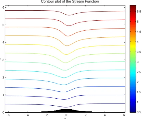
Here we used the fact that the Hilbert transform of a constant is zero andx¯=x. For comparison purpose Figs. 1 and 2 present the solutions of Eq. (45) with and without shear over this topography. We observe that in Eq. (46)ν2=GN2is not constant sinceGis a function ofx. However, in the region whereh(x)=0,G=1 and thereforeν=N. For Fig. 1,N= 1 and sinceδ=0 it follows that the base flow speedU=1, hence asymptotically (i.e. as x→ ∞)ν=1. In Fig. 2, U is not constant with height and is equal toU=1+δz; see (19). Hence the Richardson number for this flow is Ri= N2/Uz2=N2/δ2. In Fig. 2,N=1 andδ=0.1.
4 Transformations on Long’s equation with shear
x
z
Contour plot of the Stream Function
−6 −4 −2 0 2 4 6
0 1 2 3 4 5 6
0.5 1 1.5 2 2.5 3 3.5 4 4.5 5 5.5
Fig. 1. Solution of Eq. (45) over a “witch of Agnesi” topography
with=0.2,δ=0,N=1,β=µ=0.
To begin with we definez¯=z−β/2+δ/N2,x¯=x/µand substitute in Eq. (22) we obtain after dropping the bars that
ψzz−α2ψz2
+
ψxx−α2ψx2
+N2(ψ )[(1+βδ)ψ−z]=0. (49) Assuming thatN2(ψ )is constant we now apply the trans-formation
φ=e−α2ψ, α6=0. (50)
Equation (49) becomes
∇2φ+N2φα2z+(1+βδ)lnφ=0. (51) Similar transformations can be applied to the perturbation equation (34). In fact if we letx¯=x/µand introduce
χ=e−α2η, α6=0. (52)
then (34) takes the form
∇2χ−2α2(1+δz)χz+ 2α2δ+
N2 1+δz
!
χlnχ=0. (53)
We observe that|α2η| 1 thereforeχ≈1. For this reason we now introducep(x,z)=1−χ (x,z)(so that|p(x,z)| 1 again) and letln(1+x)≈xfor|x| 1. We obtain
∇2p−2α2(1+δz)pz+ 2δα2+
N2 1+δz
!
p−p2=0. (54)
x
z
Contour plot of the Stream Function
−6 −4 −2 0 2 4 6
0 1 2 3 4 5 6
1 1.5 2 2.5 3 3.5 4 4.5 5 5.5
Fig. 2. Same as Fig. 1 withδ=0.1.
However since|p(x,z)| 1 we can neglect the nonlinear terms in this equation and obtain the following linear approx-imation to Long’s equation.
∇2p−2α2(1+δz)pz+ 2δα2+
N2 1+δz
!
p=0. (55)
We observe that the only other approximation that was made in the derivation of this equation is to assume that |δη| 1. This equation is obviously superior to the usual linear approximation made in the literature withµ=0,β=0 (and δ=0).
To solve (55) we apply separation of variables and let p(x,z)=X(x)Z(z). After substitution we obtain
X(x)00+k2X(x)=0, (56)
Z(z)00−2α2(1+δz)Z(z)0+
"
2δα2+ N
2
1+δz−k
2 #
Z(z)=0 (57) wherekis a (separation of variables) constant.
z
5 10 15 20
K0.06 K0.04 K0.02 0 0.02 0.04 0.06
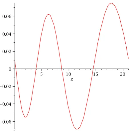
Fig. 3. A plot of of one of the solutions to (99) withN=1,δ=0.2,
α2=0.0001 andω=0.1.
plot was obtained using the numerical implementation of the Heun functions in MAPLE with a precision of 30 digits. The need to use this high precision stems from the nature of Heun functions and the roundoff errors in their evaluation (at lower precision).
4.1 Solution forδ=0
Whenδ=0 an oscillatory solution for Z(z)in (57) exists whenν2=N2−α4−k2>0 and we have
Z(z,k)=eα2z[C1(k)cosνz+C2(k)sinνz] (58)
This solution shows that the linear theory of gravity waves which is based on Eq. (39) is valid only when the modulat-ing factor eα2z is close to 1, i.e.|α2z| 1. It also shows how the wave amplitude is modulated by height due to ef-fects of stratification. In addition we note that in the standard linear theory of gravity waves the condition for oscillatory solutions isN2/U2−k2>0. This is due to the fact that this theory neglects the effect of stratification on the wave ampli-tude. (Note that in our discussion hereU=1 whenδ=0). Equation (58) can be viewed therefore as a (minor) refine-ment of this theory.
In view of (58) the general solution forp(x,z)can be writ-ten in the form
p(x,z)=
Z
√ N2−α4
−
√ N2−α4
eα2z[D1(k)cosνz+D2(k)sinνz]eikxdk
(59)
wherek is the horizontal wave number. To determine the constantsD1(k),D2(k)we have to apply the boundary
con-dition to this solution. Sinceη(x,0)has to satisfy (37) it follows from (52) and the definition ofp(x,z)that
p(x,0)=1−ef (x)=H (x). Hence
D1(k)=
1 2π
Z ∞
−∞
H (x)e−ikxdx.
To satisfy the radiation boundary condition as z→ ∞ we must insure that the vertical group velocity of the wave is positive. Using the dispersion relation for hydrostatic flow given in (Baines, 1995, p. 181) this group velocity is: cg=
N k sgn(ν)
ν2 . (60)
It follows that the vertical group velocity is positive when kν≥0.
To impose this condition on the solution (59) we re-express it in the form
p(x,z)=1 2
Z
√ N2−α4
−
√ N2−α4
h
(D1(k)−iD2(k))ei(kx+νz)
+(D1(k)+iD2(k))ei(kx−νz) i
dk . (61)
The radiation boundary condition forz→ ∞will be satis-fied if the first and second integrals vanish fork<0 andk>0 respectively. This implies that
D1(k)= −i sgn(k)D2(k). (62)
4.2 Solutions forδ1
Although Eq. (57) can be solved in terms of Heun functions it is not straightforward to delineate from this representation of the solution it general properties and apply to it the proper boundary conditions whenδ6=0. In this section we shall use proper approximations to this equation when|δz| 1 in or-der to obtain a representation of the solution in terms of ele-mentary functions. When|δz| 1 we can approximate1+1δz by(1−δz)and Eq. (57) becomes
Z(z,k)00−2α2(1+δz)Z(z,k)0
+h2δα2+N2(1−δz)−k2iZ(z,k)=0. (63) We note that the solution of this equation can be expressed in term of Kummar functions. However to derive an approx-imate representation of the solution in terms of elementary functions we have to use a first order regular perturbation ex-pansion ofZ(z)in terms ofδviz we let
Substituting this expression in (63) we obtain for the zero and first orders inδ
Z0(z,k)00−2α2Z0(z,k)0+
N2−k2Z0(z,k)=0, (65)
Z1(z,k)00−2α2Z1(z,k)0+(N2−k2)Z1(z,k)
=N2z−2α2Z0(z,k)+2α2zZ0(z,k)0. (66)
Equation (65) is the same as (57) whenδ=0 and therefore the solution forZ0(z,k)is given by (58). Substituting this
solution in (66) we find that the general solution forZ1(z)is
Z1(z)=eα
2z
[(C3+w1(z))cosνz+(C4+w2(z))sinνz] (67)
where ¯ w1(z)=
1 4ν
h
2C2α2ν−C1
N2+2α4iz2
+ 1
8ν3 n
2νhC2
N2+2α4+6C1α2ν i
z
+ C1
N2+2α4−6C2α2ν o
(68)
¯ w2(z)=
1 4ν
h
2C1α2ν+C2
N2+2α4iz2
+ 1
8ν3 n
2νhC1
N2+2α4−6C2α2ν i
z
− 6C1α2ν−C2
N2+2α4o (69)
The general solution forp(x,z)can be written as p(x,z)
=
Z
√ N2−α4
−
√ N2−α4
eα2zA(k){[C1(k)+δ (C3(k)+ ¯w1(z))]cosνzdk
+[C2(k)+δ (C4(k)+ ¯w2(z))]sinνz}eikx. (70)
Introducing the lumped constantsD1(k)=A(k)C1(k),
D2(k)=A(k)C2(k),D3(k)=A(k)C3(k),
D4(k)=A(k)C4(k)this solution can be rewritten as
p(x,z)
=
Z
√ N2−α4
−
√ N2−α4
eα2z{[D1(k)+δ (D3(k)+w1(z))]cosνzdk
+[D2(k)+δ (D4(k)+w2(z))]sinνz}eikx
=p0(x,z)+δp1(x,z), (71)
where w1(z)=
1 4ν
h
2D2α2ν−D1
N2+2α4iz2
+ 1
8ν3 n
2νhD2
N2+2α4+6D1α2ν i
z
+D1
N2+2α4−6D2α2ν o
(72) w2(z)=
1 4ν
h
2D1α2ν+D2
N2+2α4iz2
+ 1
8ν3 n
2νhD1
N2+2α4−6D2α2ν i
z
−6D1α2ν−D2
N2+2α4o.
(73) The constantsD1(k),D2(k), are determined by the same
pro-cedure used in the previous section. To determineD3we
ap-ply the boundary conditionp1(x,0)=0 which implies that
D3(k)= −
1 8ν3
h
D1(k)
N2+2α4−6D2(k)α2ν i
. (74) To determineD4we apply the radiation boundary condition
to the wave part ofp1(x,z). This yields,
D3(k)= −isgn(k)D4(k). (75)
5 Gravity waves generation in the presence of shear
To determine the effect of shear (vizδ6=0) on the solution for Z(z) in general and its oscillatory nature we shall ap-ply Sturm-Picone oscillation theorems (Sturm, 1836; Picone, 1909). To this end we write (57) in self-adjoint form
d dz
e−α2z+δz2/2dZ dz
+
"
2δα2+ N
2
1+δz−ω
2 #
e−α2 z+δz2/2
Z=0 (76)
For second order linear differential equations in this form a variant of Sturm comparison theorem states the following:
Theorem (Sturm) Assume that on the interval 0≤z≤ Zmaxthe functionsKandGin the differential equation
d dz
K(z)dy(z) dz
−G(z)y(z)=0 (77)
satisfy the inequalities
A1≥K(z)≥A2>0, B1≥G(z)≥B2. (78)
Then
2. IfB2<0 and
−B2 A2
< π
2
Z2 max
(79) then the solutions of (77) are non-oscillatory.
3. A sufficient condition for the solutions of (77) to be os-cillatory with at leastmzeroes on 0≤z≤Zmaxis
−B1 A1
≥m
2π2
Z2 max
(80)
For (76)
K(z)=e−α2 z+δz2/2
(81) and
G(z)= −
"
2δα2+ N
2
1+δz−ω
2 #
e−α2 z+δz2/2
(82)
It is obvious that we can choose A1=1 and A2=
e−α2 Zmax+δZmax2 /2
. To findB1,B2we rewrite the second
in-equality in (78) as
−B1≤ −G(z)≤ −B2. (83)
It is easy to see then that a proper choice of these constants is
B1= − "
2δα2+ N
2
(1+δZmax)
−ω2
#
e−α2 Zmax+δZ2max/2
(84)
B2= −
N2+2δα2−ω2 (85)
From the first item in the list above we obtain that the so-lution is non-oscillatory if
N2+2δα2−ω2
<0 (86)
From (79) we obtain that the solution is non-oscillatory if 0<
N2+2δα2−ω2
< π
2
Z2 max
e−α2 Zmax+δZmax2 /2
(87) Finally a sufficient condition for the solutions to oscillate and have at leastmzeroes is
"
N2 (1+δZmax)
+2δα2−ω2
#
e−α2 Zmax+δZmax2 /2
>m
2π2
Z2 max
(88) We conclude then that a sufficient condition for oscillation to exist on the interval[0,Zmax]is that
"
N2 (1+δZmax)
+2δα2
#
> π
2
Z2 max
eα2 Zmax+δZ2max/2
. (89)
Z(z)is not oscillatory if
N2+2δα2< π
2
Z2 max
e−α2 Zmax+δZ2max/2
. (90)
We infer therefore that the existence of shear will dampen the possible existence (or creation) of gravity waves since it main effect will be to decrease the value of the left hand side in (89) and increase the value of the right hand side. We observe that these results are valid for any solution of (57) and therefore especially for the solution that satisfies the boundary conditions.
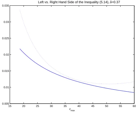
As a specific illustration of the possible effect of shear on the generation of gravity waves we consider the inequality (89) forN=0.4, β=0.025 withδ=0 (no shear) andδ= 0.37 as a function ofZmax(these values of the parameters
are relevant in atmospheric studies). In Figs. 4 and 5 we plotted the values of the left hand side of the inequality (solid line) versus the values of the right side (dotted line) for these two values ofδ. We see that when no shear is present the inequality (89) is satisfied forZmax>8 but it is not satisfied
for any value ofZmaxfor the case with shear. We infer then
that under these circumstances gravity waves will be present if the base flow is shearless but no such waves will be present if the base flow contains a strong enough shear component. This result is in line with other investigations on the effect of shear on gravity waves in the atmosphere (Shutts, 2006; Dewan, 1998).
6 Pure shear flow
In the previous sections we considered a base flow which satisfies (19) with 0≤δ1. In this section we consider the “pure shear” case where
ψ (−∞,z)=z2. (91)
In this caseu(−∞,z)=z that isu increases linearly with height. Using (14) we find that
S(ψ )=2−N2(ψ )hψ1/2+2βψi (92) and Long’s equation (14) forψbecomes
ψzz−α2ψz2
+µ2ψxx−α2ψx2
−N2(ψ )z
=2−N2(ψ )hψ1/2+2βψi. (93)
To derive an equation for a perturbation from the base flow we setψ=z2+η(x,z)and substitute in (93)
ηzz−α2ηz2
+µ2ηxx−α2ηx2
−4α2(zηz−η)
−N2z+N2
q
0 10 20 30 40 50 60 0
0.1 0.2 0.3 0.4 0.5 0.6 0.7 0.8
z
max
Left vs. Right Hand Side of the Inequality (5.14), δ=0
Fig. 4. A plot of the left hand of the inequality (89) (solid line)
versus the right hand side (dotted line) whenN=0,β=0.025 and
δ=0 as a function ofZmax.
For|η| zwe can approximate the square root in this equa-tion bypz2+η≈z+η/(2z). This leads to
ηzz−α2η2z
+µ2
ηxx−α2ηx2
−4α2(zηz−η)+
N2 2zη=0.
(95) On this equation we now apply the transformationx¯=x/µ and then apply (52). We obtain
∇2χ−4α2zχz+
N2 2z+4α
2 !
χlnχ=0. (96)
Using the arguments which proceeded (54) and (55) we in-troducep(x,z)=1−χ (x,z) and neglect the second order terms inp. This yields,
∇2p−4α2zpz+
N2 2z +4α
2 !
p=0. (97)
This equation can be solved by separation of variables. In-troducingp(x,z)=X(x)Z(z)we obtain forX(x)(56) and forZ(z)the following
Z(z)00−4α2zZ(z)0+ N
2
2z +4α
2−ω2 !
Z(z)=0 (98)
The general solution of this equation can be expressed in term of Heun functions. To determine under what conditions this solution is oscillatory we rewrite (98) in the following form
d dz
e−2α2z2dZ dz
+ N
2
2z+4α
2z−ω2 !
e−2α2z2Z(z)=0 (99)
15 20 25 30 35 40 45 50 55 60
0.005 0.01 0.015 0.02 0.025 0.03 0.035
zmax
Left vs. Right Hand Side of the Inequality (5.14), δ=0.37
Fig. 5. Same as Fig. 4 withδ=0.37.
and apply Sturm theorem on the interval[z0,Zmax](wherez0
is determined by the requirement that|η| z0). In this case
A1=e−2α
2z2
0andA2=e−2α2Zmax2 . Similarly B1= −
N2 2Zmax
+4α2z0−ω2 !
e−2α2Z2max
B2= −
N2 2z0
+4α2Zmax−ω2 !
e−2α2z20
We infer therefore that the solution will not be oscillatory if either
N2 2z0
+4α2Zmax−ω2 !
<0, or
0< N
2
2z0
+4α2Zmax−ω2 !
< π
2
Z2 max
e2α2z20−Zmax2
.
Finally a sufficient condition for the solution to oscillate and has at leastmzeroes if
N2 2Zmax
+4α2z0−ω2 !
e−2α2Zmax2 >m
2π2
Z2 max
e−2α2z20 (100) We conclude then that a sufficient condition for an oscillation to exist on the interval[z0,Zmax]is that
N2 2Zmax
+4α2z0 !
> π
2
Zmax2 e
2α2 Z2max−z20
. (101)
Z(z)is not Oscillatory if N2
2z0
+4α2Zmax<
π2 Z2
max
e2α2 z20−Zmax2
7 Summary and conclusions
We derived in this paper the proper form of Long’s equation with shear. Using a sequence of transformations and mild approximations which conserve the geophysical contents of this equation we were able to deduce some criteria for the excitation of gravity wave under these conditions. These criteria depend only the shear contents in the base flow, the value of N2 and the stratification. These results will be useful both experimentally and theoretically. Currently the experimental practice is to ignore the shear in the base flow (Shutts et al., 1988; Vernin et al., 2007) and attempt to deduce the quantitative attributes of the gravity waves using the shearless Long’s equation. As a result several models for the generation of gravity waves overestimate their production. These models can be refined now by taking this important feature into account.
Edited by: R. Grimshaw
Reviewed by: two anonymous referees
References
Baines, P. G.: Topographic effects in Stratified flows, Cambridge Univ. Press, New-York, 1995.
Nappo, C. J.: Atmospheric Gravity Waves, Academic Press, Boston, 2002.
Davis, K. S.: Flow of Nonuniformly Stratified Fluid of Large Depth over Topography. M.Sc. thesis in Mechanical Engineering, MIT, Cambridge, MA, 1999.
Dewan, E. M., Picard, R. H., O’Neil, R. R., Gardiner, H. A., Gib-son, J., Mill, J. D., Richards, E., Kendra, M., and Gallery, W. O.: MSX satellite observations of thunderstorm-generated grav-ity waves in mid-wave infrared images of the upper stratosphere, Geophys. Res. Lett., 25(7), 939–942, 1998.
Doyle, J. D., Volkert, H., Dornbrac, A., Hoinka, K. P., and Hogan, T. F.: Aircraft measurements and numerical simulations of moun-tain waves over the central Alps: A pre-MAP test case, Q. J. Roy. Meteor. Soc., 128, 2175–2184, 2006.
Drazin, P. G.: On the steady flow of a fluid of variable density past an obstacle, Tellus, 13, 239–251, 1961.
Drazin, P.G. and Moorem, D. W.: Steady two dimensional flow of fluid of variable density over an obstacle, J. Fluid. Mech., 28, 353–370, 1967.
Dubreil-Jacotin, M. L.: Sur la determination rigoureuse des ondes permanentes periodiques d’ampleur finie, J. Math. Pure. Appl., 13, 217–291, 1934.
Durran, D. R.: Two-Layer solutions to Long’s equation for verti-cally propagating mountain waves, Q. J. Roy. Meteor. Soc., 118, 415–433, 1992.
Eckermann, S. D. and Preusse, P.: Global measurements of strato-spheric mountain waves from space, Science, 286, 1534–1537, 1999.
Humi, M.: On the Solution of Long’s Equation Over Terrain, Il Nuovo Cimento C, 27, 219–229, 2004a.
Humi, M.: Estimation of Atmospheric Structure Constants from Airplane Data, J. Atmos. Ocean. Tech., 21, 495–500, 2004b. Humi, M.: On the Solution of Long’s Equation with Shear, Siam J.
Appl. Math., 66(6), 1839–1852, 2006.
Humi, M.: Density representation of Long’s equation, Nonlin. Pro-cesses Geophys., 14, 273–283, 2007,
http://www.nonlin-processes-geophys.net/14/273/2007/. Humi, M.: Long’s equation in terrain following coordinates,
Non-lin. Processes Geophys., 16, 533–541, 2009,
http://www.nonlin-processes-geophys.net/16/533/2009/. Lily, D. K. and Klemp, J. B.: The effect of terrain shape on
non-linear hydrostatic mountain waves, J. Fluid Mech., 95, 241–261, 1979.
Long, R. R.: Some aspects of the flow of stratified fluids I. Theoret-ical investigation, Tellus, 5, 42–57, 1953.
Long, R. R.: Some aspects of the flow of stratified fluids II. Theo-retical investigation, Tellus, 6, 97–115, 1954.
Long, R. R.: Some aspects of the flow of stratified fluids III. Con-tinuous density gradients, Tellus, 7, 341–357, 1955.
Long, R. R.: The motion of fluids with density stratification, J. Geo-phys. Res., 64, 2151–2163, 1959.
Miropol’sky, Yu. Z.: Propagation of internal waves in an ocean with horizontal density field non-uniformities, Izv. Atmos. Ocean. Phy+, 10, 312–318, 1974.
Miropol’sky, Yu. Z.: Dynamics of Internal Gravity waves in the Ocean, Kluwer, Boston, 2001.
Peltier, W. R. and Clark, T. L.: Nonlinear mountain waves in two and three spatial dimensions, Q. J. Roy. Meteor. Soc., 109, 527– 548, 1983.
Picone, M.: Sui valori eccezionali di un parametro da cui dipende un’equazione differenziale lineare del secondo ordine, Ann. Scuola Norm. Sup. Pisa, 11, 1–141, 1909 (in Italian).
Shutts, G. J., Kitchen, M., and Hoare, P. H.: A large amplitude gravity wave in the lower stratosphere detected by radiosonde, Q. J. Roy. Meteor. Soc., 114, 579–594, 1988.
Shutts, G. J., Healey, P., and Mobbs, S. D.: A multiple sounding technique for the study of gravity waves, Q. J. Roy. Meteor. Soc., 120, 59–77, 1994.
Shutts, G. J.: Stationary gravity-wave structure in flows with di-rectional wind shear, Q. J. Roy. Meteor. Soc., 124, 1421–1442, 1998.
Smith, R. B.: Linear theory of stratified hydrostatic flow past an isolated mountain, Tellus, 32, 348–364, 1980.
Smith, R. B.: Hydrostatic airflow over mountains, Adv. Geophys., 31, 1–41, 1989.
Sturm, J. C. F.: Sur les equations differenielles lineares du second ordre, J. Math. Pure Appl., 1, 106–186, 1836 (in French). Vernin, J., Trinquet, H., Jumper, G., Murphy, E., and Ratkowski, A.:
OHP02 gravity wave campaign in relation to optical turbulence, Environ. Fluid Mech., 7, 371–382, 2007.
Yih, C.-S.: Equations governing steady two-dimensional large am-plitude motion of a stratified fluid, J. Fluid Mech., 29, 539–544, 1967.