A Lagrangian approach to the Loop Current eddy separation

(1)

Nonlin. Processes Geophys., 20, 85–96, 2013 www.nonlin-processes-geophys.net/20/85/2013/ doi:10.5194/npg-20-85-2013

Nonlinear Processes

in Geophysics

A Lagrangian approach to the Loop Current eddy separation

F. Andrade-Canto1, J. Sheinbaum1, and L. Zavala Sans´on1

1_{Departmento de Oceanograf´ıa F´ısica, CICESE, Carretera Ensenada-Tijuana 3918, 22860 Ensenada, Baja California, M´exico} Correspondence to: F. Andrade ([email protected])

Received: 12 April 2012 – Revised: 27 October 2012 – Accepted: 14 December 2012 – Published: 23 January 2013

Abstract. Determining when and how a Loop Current eddy (LCE) in the Gulf of Mexico will finally separate is a diffi-cult task, since several detachment re-attachment processes can occur during one of these events. Separation is usually defined based on snapshots of Eulerian fields such as sea sur-face height (SSH) but here we suggest that a Lagrangian view of the LCE separation process is more appropriate and ob-jective. The basic idea is very simple: separation should be defined whenever water particles from the cyclonic side of the Loop Current move swiftly from the Yucatan Peninsula to the Florida Straits instead of penetrating into the NE Gulf of Mexico. The properties of backward-time finite time Lya-punov exponents (FTLE) computed from a numerical model of the Gulf of Mexico and Caribbean Sea are used to estimate the “skeleton” of flow and the structures involved in LCE de-tachment events. An Eulerian metric is defined, based on the slope of the strain direction of the instantaneous hyperbolic point of the Loop Current anticyclone that provides useful information to forecast final LCE detachments. We highlight cases in which an LCE separation metric based on SSH con-tours (Leben, 2005) suggests there is a separated LCE that later reattaches, whereas the slope method and FTLE struc-ture indicate the eddy remains dynamically connected to the Loop Current during the process.

1 Introduction

One of the most interesting features of the circulation in the Gulf of Mexico (GoM) is the Loop Current (LC). The LC can either extend deep into the northeast GoM (24–28◦N) and turn clockwise back to Cuba and the Florida Straits, or go directly from the Yucatan Channel to the Florida Straits (Candela et al., 2002; Leben, 2005). The LC is well known for shedding large anticyclones (Loop Current Eddies, LCEs) at irregular intervals between 0.5–18.5 months (Sturges and

Leben, 2000), which travel westward across the GoM. These eddies decay in the central Gulf from interaction with other eddies (Lipphardt et al., 2008), or reach the western slope of the GoM and decay by interaction with topography generat-ing coastal currents and eddies (Sturges, 1994).

Although the mechanisms and frequency of LCE shed-ding have been studied by many authors, critical aspects of the process remain uncertain (Alvera-Azcarate et al., 2009; Maul and Vukovich, 1993; Sturges, 1994; Vukovich, 1995). Some authors have discussed several events where small cy-clonic eddies on the periphery of the Loop Current influ-ence the shedding of the LC rings (Fratantoni et al., 1998; Zavala-Hidalgo et al., 2003; Ch´erubin et al., 2006; Schmitz, 2005). Using 3 yr of direct mooring observations together with altimetry data Athi´e et al. (2011) find that some shed-ding events are associated with cyclonic anomalies coming from the Caribbean producing an eastward shift of the LC core. Downstream from the LC, Sturges et al. (2010) finds perturbations in the transport measurements from the cable between Miami and the Bahamas that precede several LCE detachments. All these findings suggest the detachment pro-cess is quite complicated, more so, since eddies may fre-quently detach and reattach from the LC during intrusion into the GoM.

(2)

86 F. Andrade-Canto et al.: A Lagrangian approach to eddy separation

F. Andrade-Canto et al.: LALCES

9 Fig. 01.

Weekly snapshot of SSH from AVISO (Panel a), and SST from GOES SST composite produced by Louissiana State University

(Panel b), for Feb. 6, 2008. Notice the

17 −

SSH

contour (black line) suggests the Loop Current Eddy (LCE) has already dettached from

the LC whereas the SST composite indicates the LCE is still attached

Fig. 02.

Weekley snapshots of SSH field in

m

for an LCE detachment-reattachment event that occurred in May-June 2008 obtained from

AVISO data. Once a separation occurs, the

17 −

SSH

contour does not provide information on whether or not there will be a later

reattach-ment as it happens in this event.

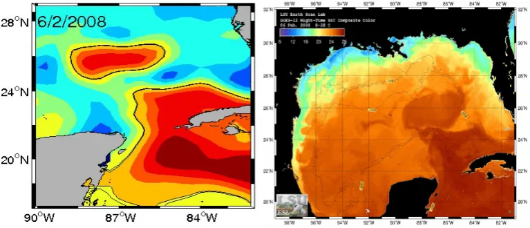
Fig. 1. Weekly snapshot of SSH from AVISO (Archiving, validation and interpretation of satellite oceanographic data) (a), and SST from GOES (Geostationary Operational Environmental Satellite) SST composite produced by Louisiana State University (b), for 6 February 2008. Notice the 17-SSH contour (black line) suggests the Loop Current eddy (LCE) has already detached from the LC whereas the SST composite indicates the LCE is still attached.

suggests the LCE is still attached. Similarly, Fig. 2 shows snapshots of a shedding event highlighting the 17-SSH con-tour (data computed from AVISO satellite altimetry data, http://www.aviso.oceanobs.com), showing the extension of the LC into the GoM (left panel). A detached LCE is depicted in the middle panel, but, as already mentioned, there is no in-dication in this SSH field that the eddy would reattach later on, as it happened in this case (right-hand panel). Visual anal-ysis of figures like these might indicate the moment when the shedding begins, but the method does not capture the details of how the process takes place and makes it difficult to de-termine the final moment of detachment. One reason for this is related to the fact that SSH maps provide an Eulerian view of what is basically a Lagrangian process (Haller, 2005). Be-sides, since the flow is time-dependent, the SSH field, which plays the role of stream-function for surface geostrophic ve-locities (in the quasi-gesotrophic framework), does not indi-cate particle paths in general. Thus, it makes sense to analyze the separation process from a Lagrangian point of view.

Kuznetsov et al. (2002) used near-surface currents from a numerical model and computed material lines to elucidate the interaction between the LC and adjacent eddies. They showed that Lagrangian analysis provides more information about the separation process than the Eulerian point of view, since the Lagrangian approach allows to determine barriers of transport between the rings and the surrounding fluid as-sociated with hyperbolic (saddle) regions in the flow. The evolution and geometry of these manifolds or distinguished material lines provide more information about the separation than the tracking of closed streamlines or vorticity contours in the Eulerian approach. Kuznetsov et al. (2002) suggest that a necessary condition for an LCE separation is the presence of a hyperbolic saddle point below the Loop Current bulge (LCB) and other flow structures. Here we refer to the LCB

as the structure that will become the LCE after separation but remains attached or is part of the Loop Current before sepa-ration occurs. Lagrangian analysis has also been used to ex-plore vortex pinch-off in laboratory experiments (O’Farrell and Dabiri, 2010) by computing finite time Lyapunov ex-ponents (FTLEs) and identifying Lagrangian coherent struc-tures (LCS). They show that the emergence of new and dis-connected LCS from the original or initial LCS that defines the vortex marks the start of the pinch-off process.

In a more recent study, (Branicki and Kirwan, 2010) per-formed a very detailed 3-D Lagrangian analysis of an LCE (eddy Juggernaut) using FTLEs and defining the eddy bound-aries as the intersection of the stable and unstable manifolds of two distinct distinguished hyperbolic trajectories (as de-fined in Mancho et al., 2006). Lobe dynamics and the so-called turnstile mechanism is used to determine the exchange of fluid between the eddy and its surroundings.

These ideas lead us to propose an alternative method to study the LC shedding process based on particle trajectories whose behaviour can be understood using structures identi-fied in FTLE diagnostics that participate in the LCE sepa-ration. In contrast to the detailed analysis of Branicki and Kirwan (2010) and Kuznetsov et al. (2002), our interest is perhaps less ambitious, and is simply to define a Lagrangian LCE separation index that will indicate when fluid particles on the cyclonic side of the LC move directly to the east (Florida Straits) instead of around the LCB inside the GoM. This criterion is objective (i.e., frame independent), and in fact, does not require a precise definition of the LCE bound-ary, an issue thoroughly analyzed in Branicki and Kirwan (2010). Our hope is that by developing an index that captures part of the Lagrangian aspects of the LCE separation, we will obtain more reliable information about the process than the

(3)

F. Andrade-Canto et al.: A Lagrangian approach to eddy separation 87

F. Andrade-Canto et al.: LALCES

9

Fig. 01. Weekly snapshot of SSH from AVISO (Panel a), and SST from GOES SST composite produced by Louissiana State University (Panel b), for Feb. 6, 2008. Notice the17−SSH contour (black line) suggests the Loop Current Eddy (LCE) has already dettached from the LC whereas the SST composite indicates the LCE is still attached

Fig. 02. Weekley snapshots of SSH field inmfor an LCE detachment-reattachment event that occurred in May-June 2008 obtained from AVISO data. Once a separation occurs, the17−SSH contour does not provide information on whether or not there will be a later reattach-ment as it happens in this event.

Fig. 2. Weekly snapshots of the SSH field in m for an LCE detachment–reattachment event that occurred in May–June 2008 obtained from AVISO data. Once a separation occurs, the 17-SSH contour does not provide information on whether or not there will be a later reattachment, as it happened in this event.

one provided by snapshots of Eulerian fields such as those based on SSH (Leben, 2005).

To test these ideas we use numerical model output, so the FTLE fields are computed using velocity data from a numer-ical simulation of the circulation in the Caribbean Sea and GoM based on the NEMO (Nucleus for European Modelling of the Ocean) model (Jouanno et al., 2009). Eight LCE sep-aration cases were analyzed and compared using both the FTLE technique and Leben’s SSH contour method (Leben, 2005). The FTLE field was computed for each day, using ve-locities at a depth of 68 m. Analysis of the FTLE highlights some geometric structures in the flow that actively participate in the detachment process. Although a strictly Lagrangian separation index is not defined, we found that LCB instan-taneous hyperbolic saddle points and their strain direction (an Eulerian calculation) provide information consistent with FTLE features such as their local orientation near the stagna-tion point. An index is defined based on these observastagna-tions and indicates the orientation of such instantaneous strain di-rections. It appears to capture the change in particle paths before separation and provides a useful criterion to identify – even predict – that final LCE detachments are about to oc-cur. The LCE separation cases discussed here have particular characteristics that represent several other separation events. By contrasting the FTLE method and Leben’s SSH method, we aim to clarify their benefits and limitations.

The paper is organized as follows: Sect. 2 briefly describes the concept of Lagrangian coherent structures, the FTLE method used to obtain them and the data employed to com-pute the FTLE fields. Section 3 describes the analysis of the FTLE field and develops the new Eulerian metric for LCE separation status based on the local strain orientation; this criterion is compared to the 17-SSH altimetry method. It is shown that the new method is better at determining when the final LCE separation will occur. Section 4 is the summary and conclusions. Appendix A provides mathematical details of some of the calculations.

2 FTLE

We use the developed concept of LCS (Haller, 2001a), for example, as regions (or structures of dimensionn−1, where

nis the spatial dimension of the flow field) in unsteady flows based on their stability properties in finite time, which can be roughly detected by looking at the maxima of the finite time Lyapunov exponent diagnostic (see below). The LCS can be considered a generalization of the stable and unsta-ble manifolds using their physical property of being respec-tively the most repelling and attracting structures for particles located normal to them. Although, in general, they are not strictly material lines (Haller, 2001b and Branicki and Wig-gins, 2009), in many instances they provide good approxi-mations to actual material structures (as in the LCE separa-tion problem, see Branicki and Kirwan, 2010). LCS define the boundary between fluid domains of different dynamical characteristics, but in contrast to steady flows, attracting and repelling LCS can intersect each other many times forming lobes, which allow fluid exchange between eddies and the exterior. The study of LCS allows identification of transport barriers, transport mechanisms, and regions of rapid disper-sion (Beron-Vera et al., 2008; Shadden et al., 2005, 2006; Mathur et al., 2007; Mancho et al., 2006)

The FTLE method is a useful technique for estimating LCS (Haller, 2001a, 2002; Shadden et al., 2005, 2006; Olas-coaga et al., 2006; Lekien and Coulliette, 2007; Lekien et al., 2005, 2007; Mathur et al., 2007) since it provides a measure of the maximum separation rate of initially nearby fluid par-ticles in a finite time. It can be employed in any number of dimensions (Lekien and Coulliette, 2007) but here we focus on the 2-D case. Ifx0=(x0, y0)denotes the initial position on a 2-D space of a fluid particle at timet0, its position at any time t, denotedx(t;x0, y0), follows by integrating the trajectory equation:

˙

x=u(x, t ), (1)

where the overdot stands for time differentiation, andu=

(4)

σ_tT

0 = 1

2|T |lnλmax(1), (2)

whereλmaxdenotes the maximum eigenvalue of1, the finite time Cauchy-Green deformation tensor:

1(t;x0, t0):=∂x0x(t;x0, t0)

∗

∂x0x(t;x0, t0), (3) where∗denotes the transpose.

Maps of FTLE are computed by calculating Eqs. (2) and (3) upon estimation of∂x0x(t0+T;x0, t0)by direct finite dif-ferentiation of fluid particle trajectories with initial positions distributed on a regular grid.The calculations are performed by using the MANGEN (Manifold Generator) software, a dy-namical systems tool-kit designed by F. Lekien and C. Coul-liette. Regions of maximum separation rates produce ridges in the FTLE field that approximate attracting (repelling) LCS when integrating particle trajectories backward (forward) in time. Repelling and attracting LCS delineate the boundary between fluid regions with distinct flow characteristics.

The velocity field used to compute the FTLEs is daily model velocity output from a numerical simulation based on Jouanno et al. (2009), in which the NEMO-AGRIF (adap-tive mesh refinement software) model was implemented for the Caribbean Sea and GoM (98◦W–57◦W, 6◦N–31◦N). This configuration is a nested grid model with a horizon-tal resolution of 1/15 degree (approximately 7 km) em-bedded in a coarser grid eddy-permitting (1/3 degree, ap-proximately 35 km resolution) North Atlantic configuration (50◦_N–20◦_{S). Both, the coarse and fine resolution grids}

have 46 vertical levels whose spacing increases from 12 m at the surface to 250 m below 1500 m. The two grids inter-act in both ways using the AGRIF methodology (Debreu, 2000), i.e., the fine grid solution also impacts the solution in the coarse grid. By contrast with the simulation reported in Jouanno et al. (2009), which uses climatological surface forcing, the simulation used here is a 40 yr integration (1958– 2006, 9 yr spin-up) carried out with interannual forcing from the ERA40 reanalysis corrected by Brodeau et al. (2010). As discussed in Jouanno et al. (2009), the model reproduces the mean circulation and eddy characteristics in the region. Al-though Jouanno et al. (2009) do not discuss the circulation in the GoM, preliminary results of the inter-annual run (1958– 2006) by Sheinbaum et al. (2010) indicate the simulation of LC eddy shedding events required for the present study are consistent with observations.

The daily output of velocity and SSH fields corresponds to years 1997 to 2005 in which we identified eight shedding events. The basic difference among them is whether or not one or several reattachments occur once an LCE separates. The following discussion focuses particularly on two of the eight events analyzed in which this difference is more evi-dent. The initial separation time in all events is first identified from the model SSH field.

The velocity used to advect the particles corresponds to the sixth vertical level of the model at 68 m depth. This depth is chosen close to the surface but at the same time below the mean mixed layer depth so that some ageostrophic compo-nents are partially filtered out to facilitate future comparison of the results with those obtained from surface geostrophic velocities from altimetry data. Results, however, are similar if a shallower level is chosen (not shown). The vertical veloc-ity at this depth is not exactly zero, but sufficiently small that horizontal velocities can be approximated as non-divergent. Several studies (Olascoaga et al., 2006; Kuznetsov et al., 2002) suggest that this is a reasonable approximation which properly describes transport processes for the space and time scales relevant to the LCE separation. According to Branicki and Kirwan (2010) this assumption is valid if the product of

H is much smaller than unity, whereis the average vertical shear in a fluid layer of thicknessH divided by the average horizontal velocity. As in Branicki and Kirwan (2010), we find the criterion is satisfied in a layer about 150–200 m wide (from the surface) sinceH 1, which supports the original assumption.

Particle trajectories are determined using a time-step-adapting fourth/fifth-order Runge–Kutta method scheme with a fixed 1h time step and a tricubic method for the re-quired spatio-temporal interpolation of the numerically gen-erated velocity field to the particle positions. The initial par-ticle “grid” is four times finer than the velocity grid and is composed of 1000×1000 particles. To evaluate Eq. (2), MANGEN uses central differences and standard eigenvalue solvers, see Shadden et al. (2005); Lekien and Coulliette (2007) for details. Daily FTLE maps are computed for a period of 30 days, advecting particles backward in time 35 days, i.e., integrating Eq. (1) fromt (i)tot (i−35), where

i=1,2, . . .30 indicates starting day of integration. This pe-riod captures the shedding events including detachments and reattachments if they occur, and also keeps a large number of the initial particles in the region of interest. The attracting– repelling properties of the LCSs change with time and are only valid for the period they are calculated from. This means that results could change if a different integration period is employed (Branicki and Kirwan, 2010), and in fact, some structures may even change their properties within the time interval used in their computation. Recent work defines LCS cores (Olascoaga and Haller, 2012) as structures that pre-serve their attracting–repelling character during the whole interval. Our FTLE analysis is qualitative and such detailed calculations are not needed. In that sense, we find that results are not sensitive to slight modifications of the integration pe-riod (even if it is extended to 50 days, similar features in the FTLE diagnostics, their character and evolution are identi-fied, see below).

(5)

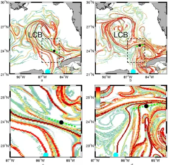
Fig. 3. Snapshots of FTLE field in d−1computed backward in time for 35 days, for 1 June (a) and 30 June (b) of model simulation year 2000. Regions of red tones indicate the possible attracting LCSs (ridges). These images show the Loop Current Bulge (LCB) in conditions where the LCB is attached (a) and separating (b). Both panels show the instantaneous hyperbolic point (black dot) computed from the “frozen” velocity field of each day together with its strain direction (dashed green segment), named LCBsd in the text. The cyan dot marks the origin of a ridge on the western side of the Yucatan Ridge (YR), which plays an important role in the separation process. To better appreciate the ridges involved, (c) and (d) zoom into the region indicated by rectangles shown in (a) and (b) (see text for details).

3 Results

Figure 3 shows the FTLE fields computed backward in time for 35 days for 1 June (Fig. 3a) and 30 June 2000 (Fig. 3b). The regions with intense red tones indicate maximum val-ues of the FTLEs and identify possible attracting LCS, so we refer to them simply as ridges. This is a rough estimate but sufficient for our calculations, since properties of the identi-fied FTLE ridge structures are corroborated a posteriori by looking at the behaviour of particles (see below). Notice that ridges in the FTLE field not necessarily represent hyper-bolic LCSs, as they may correspond to regions of high shear (Haller, 2011).

The two top panels depict a full view of the FTLE field. Several highly complex and entangled structures are ob-served, but some particular coherent features relevant to the LCE separation can be identified. These are discussed below using Fig. 3c and d, zooming into the saddle region.

In Fig. 3a and b the LCB is located close to the center of the map and can be identified by low FTLE values which are surrounded by high FTLE values. Below the LCB, a black dot marks its associated instantaneous hyperbolic point (LCBhp) and the dashed green line indicates its correspond-ing strain direction (LCBsd). The circulation in the region is such that several instantaneous stagnation points can be found at any given time, though it is not always possible to relate one of them to the LCB. The method used to locate the LCBhp is explained in the Appendix A and uses Eulerian information from SSH, and Okubo–Weiss fields. It is clear in these figures that the LCBhp is in a region surrounded by FTLE ridges and that the LCBsd (green segment) has roughly the same orientation as the FTLE ridges near the saddle point.

(6)

F. Andrade-Canto et al.: LALCES

11

Fig. 04.Snapshots of SSH field inm(top panel) and FTLE field ind−1(lower panel) for the days indicated in Figure 06a: May 19, June 9, August 9 and September 15. The SSH field in the second column shows a detached LCE while the FTLE is highly structured and the YR still wraps around the LCB. Most of the particles (blue to black dots, the color indicates the day which are settled; marked in the bottom of each snapshot) seeded on the left corner of the Yucatan Peninsula, go north following the YR (yellow triangle) indicating the eddy is still attached. Finally, in the last panel a substantial number of particles travel directly to the east following the YR, signalling that the LCE is totally separated. (see text)

Fig. 05. Snapshots of SSH field inm(top panel) and FTLE field ind−1_{(lower panel) for the days indicated in Figure 06c: Feb 21, March}

19, April 17 and May 12. SSH maps for March and April suggest the LCE separated while the FTLE maps and the particle trajectories clearly indicate there is no direct eastward intrusion of particles from the western side of the Yucatan Current until the final snapshot, where the LCE is totally separated (see text).

Fig. 4. Snapshots of SSH fields in m (top panel) and FTLE fields in d−1(lower panel) for the days indicated in Fig. 6a: 19 May, 9 June, 9 August and 15 September. The SSH field in the second column shows a detached LCE while the FTLE is highly structured and the YR still wraps around the LCB. Most of the particles (blue to black dots, the color indicates the day in which they are settled; marked in the bottom of each snapshot) seeded on the left corner of the Yucatan Peninsula go north following the YR, (yellow triangle) indicating the eddy is still attached. Finally, in the last panel, a substantial number of particles travel directly to the east following the YR, signalling that the LCE is totally separated. (see text).

the LC. We name it the Yucatan ridge (YR) from its origin, but one can see the YR marks the external rim of the LC. It extends northward surrounding the LCB and then joins the Florida Current in Fig. 3a. By contrast, in Fig. 3b the YR turns eastward and no longer wraps around the LCB which is now nearly separated from the Loop Current forming the LCE.

Differences between these two conditions of the LCE sep-aration process can be better appreciated in Fig. 3c and d, which zoom into the saddle point region marked by the square in Fig. 3a and b. In Fig. 3c, high FTLE values are vis-ible between the ridges parallel to the LCBsd and the YR in-dicating the presence of other ridges, whereas in Fig. 3d, low FTLE values are found between these two ridges. These low FTLE values are related to particles which remain together (separate less rapidly) approaching the ridges, i.e., particles which have their origin on the western (cyclonic) side of the Yucatan and Loop Currents are now moving northeastward attracted by the YR (actually nearby particles on both sides of the YR move towards it). Notice also the different ori-entations of the strain direction in the figures. The LCBsd is oriented in the northwest–southeast direction in Fig. 3a, whereas in Fig. 3b, its orientation is southwest–northeast. This change in strain direction when the LCE is about to separate was identified in the eight shedding events studied

in this work and will be used later on to define a separation index.

In Fig. 3, we find that changes in the structure of YR, as time evolves, indicate when fluid particles on the cyclonic side of the Yucatan Current will start to move eastward in-stead of going to the northwest around the LCB. This is a more reliable indicator of LCE separation than tracking a par-ticular contour of the sea surface height, simply because in a time dependent flow, particle paths are not the same as stream lines. The SSH field (streamlines for the surface flow in the quasi-geostrophic limit) may indicate that an LCE has de-tached, but particles may still move deep into the Gulf around the LCB, as will be shown below. Monitoring the YR and using it to define separation is not that simple, due to its La-grangian character.

We can, however, formulate a relatively simple LCE Eu-lerian separation index based on the observed changes in the slope of the instantaneous strain direction at the LCB hyper-bolic point, which appears to capture qualitative properties of the Lagrangian behaviour discussed above.

The lower panels in Figs. 4 and 5 show seeded parti-cles (green, black and blue colors) on top of FTLE diagnos-tics, and were obtained from snapshots of movies of FTLEs and particle trajectories in two particular events during 1997 and 2002. These animations suggest quite clearly that parti-cles are indeed attracted and follow some of the previously

(7)

F. Andrade-Canto et al.: LALCES 11

Fig. 04.Snapshots of SSH field inm(top panel) and FTLE field ind−1_{(lower panel) for the days indicated in Figure 06a: May 19, June 9,}

August 9 and September 15. The SSH field in the second column shows a detached LCE while the FTLE is highly structured and the YR still wraps around the LCB. Most of the particles (blue to black dots, the color indicates the day which are settled; marked in the bottom of each snapshot) seeded on the left corner of the Yucatan Peninsula, go north following the YR (yellow triangle) indicating the eddy is still attached. Finally, in the last panel a substantial number of particles travel directly to the east following the YR, signalling that the LCE is totally separated. (see text)

Fig. 05. Snapshots of SSH field inm(top panel) and FTLE field ind−1_{(lower panel) for the days indicated in Figure 06c: Feb 21, March}

19, April 17 and May 12. SSH maps for March and April suggest the LCE separated while the FTLE maps and the particle trajectories clearly indicate there is no direct eastward intrusion of particles from the western side of the Yucatan Current until the final snapshot, where the LCE is totally separated (see text).

Fig. 5. Snapshots of SSH fields in m (top panel) and FTLE fields in d−1(lower panel) for the days indicated in Fig. 6c: 21 February, 19 March, 17 April and 12 May. SSH maps for March and April suggest the LCE separated while the FTLE maps and the particle trajectories clearly indicate there is no direct eastward intrusion of particles from the western side of the Yucatan Current until the final snapshot, where the LCE is totally separated (see text).

identified ridges. Particularly interesting is the YR, whose evolution does seem to control how particles on the cyclonic side of the YC–LC behave. What we found, is that when the YR wraps around the LCB, marking also the movement of the seeded particles, the LCBsd has a distinctive (nega-tive) northwest–southeast orientation. A soon as the YR in-trudes to the east, this orientation begins to change until it becomes positive and strongly southwest–northeast before an LCE separation. As shown below (Fig. 6), the index’s change of sign from negative to positive does indicate that a final LCE separation will soon occur, but no particular range of values can be used to determine whether or not the eddy has separated. The fact that the LCBsd is, in general, parallel to an FTLE ridge and that one can relate it to particle move-ment, makes it a quasi-Lagrangian separation index.

The change in LCBsd orientation is calculated by locat-ing the instantaneous hyperbolic stagnation point and the eigenvalues and eigenvectors of the gradient velocity tensor for each day at the point. The slope of the LCBsd is given by the orientation of eigenvector V+ _{corresponding to the}

largest eigenvalueλ+of ∇U. Negative values indicate that the LCBsd is oriented in the northwest–southeast direction, which means the LCB is attached, whereas positive values in-dicate southwest–northeast orientation and the LCE is close to separation. Several stagnation points appear in the flow at any given time, so in order to identify the actual hyperbolic point related to the LCB, a method was developed to reduce

the uncertainty generated by the presence of other hyperbolic points (for details of all these calculations see Appendix A). It should be mentioned that finding the LCBhp is not always possible, though this only happens on few occasions.

A question also arises as to whether the time scales in-volved in these calculations and those related to the LCE separation are consistent, so as to guarantee that the fields evolve sufficiently slowly. Such a condition allows one to relate the trajectory of the instantaneous hyperbolic stagna-tion point and its velocity Jacobian eigenvalue-eigenvector pairs to the presence of a nearby Lagrangian hyperbolic tra-jectory. Although we are not interested in computing the hy-perbolic trajectory, the conditions established (Haller et al., 1997, 1998; Velasco Fuentes, 2001) that permit this connec-tion are satisfied in all separaconnec-tion cases (see Appendix A).

(8)

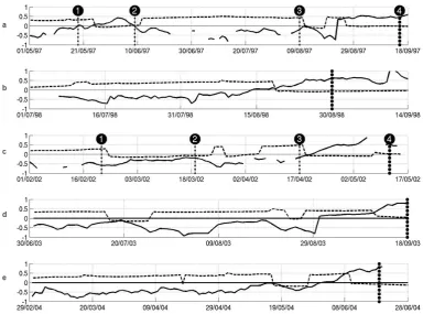
Fig. 6. Time series of two indices used to determine the LC state and LCE separation. The dashed line is the length of the 17-SSH contour whereas the continuous line depicts the LCBsd slope index. Each panel represents conditions during 5 different shedding periods of the numerical simulation corresponding to May–August 1997, June–August 1998, February–April 2002, July–September 2003, and March– June 2004, respectively. The vertical dashed line indicates the final separation date determined from analysis of the FTLE field (see text). Numbers and vertical dotted lines in (a) and (c) are explained in Figs. 4 and 5. Drops in the SSH index suggest the LCE is separated and remains in that stage as long as the value of this index remains small. The slope index indicates there will be an LCE detachment once its sign changes from negative to positive. Note that on several occasions the SSH index suggests the eddy is separated whilst the slope index indicates the eddy is still connected (see text).

vertical dotted lines indicate the time of final separation de-termined from visual inspection of the FTLE fields, and is chosen as the time when a lobe bounded by the YR (and a substantial number of seeded particles) has intruded directly east and as far as 84◦W. Numbered lines in Fig. 6a and c indicate the times of SSH and FTLE snapshots discussed in Figs. 4 and 5. The 17-SSH contour was chosen by Leben (Leben, 2005) to represent the outer boundary of the LC, so that high or increasing values of its length indicate the LC is growing, and sudden drops in its length suggest an LCE has separated.

Figure 6a, c, d, and e show various detachment– reattachment events according to this index (dashed line) and its sudden drops. By contrast, the slope index has negative values throughout several of these “detachments”, indicating there has been no separation in the Lagrangian sense. Partic-ularly interesting is the 2002 event (Fig. 6c), where the SSH index suggests the LCE separated on the third week of Febru-ary and remained so for about two months, whereas the slope index shows negative values throughout this period.

F. Andrade-Canto et al.: LALCES 13

Fig. 07.Summary of the two different stages of the Loop Current Eddy (LCE) separation process :(a) Before separation. (b) After separation. The blue lines are the streamlines, the black arrows are the velocity vectors, the black line is the LCBsd associated with the LCBhp (dot in magenta). The orientation of the strain directions is determined by the relative positions of the LCB and the LC (see text).

Fig. 08.Time evolution of the strength of the hyperbolicityλ2

2,1(thick lines), and its rate of changeλ01,2(thin lines). The computations were

made for the evolution of the LCBph2001event.

Fig. 7. Summary of the two different stages of the Loop Current eddy (LCE) separation process: (a) before separation; (b) after sep-aration. The blue lines are the streamlines, the black arrows are the velocity vectors, the black line is the LCBsd associated with the LCBhp (dot in magenta). The orientation of the strain directions is determined by the relative positions of the LCB and the LC (see text).

(9)

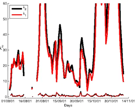
Fig. 8. Time evolution of the strength of the hyperbolicity λ2₂_,₁ (thick lines), and its rate of changeλ0₁_,₂(thin lines). The compu-tations were made for the evolution of the LCBph 2001 event.

To demonstrate that the slope index provides a closer in-dication of Lagrangian LCE separation, we analyze in more detail the 1997 and 2002 separation events by looking at dif-ferent snapshots of the SSH, and FTLEs in Figs. 4 and 5, for the days marked in Fig. 6a and c. Besides this, passive par-ticles were seeded on the west side of the Loop Current and advected by the flow. Their position is plotted together with the FTLEs to corroborate the interpretation of the computed ridges, as structures that attract nearby particles and form the “skeleton” of the flow.

In Fig. 4, the second column of panels corresponding to snapshot 2 (9 June 1997), shows that while the SSH field depicts a separated eddy (top panel), the FTLE field (lower panel) is highly structured and the YR marked by the yel-low triangle, though quite folded, ceases to wrap the LCB. Notice that some particles do cross to the east directly from Yucatan. This may be the reason why the slope index (con-tinuous line in Fig. 6a) has a positive value and yet the LCB is almost separated. Nonetheless, a movie of the process (not shown) indicates the Cuban anticyclone (the structure below the LCB) begins to decrease and this allows reattachment of the LCB. Looking now at the fourth column of panels, with conditions representing what we identify with true final LCE separation time, we see that a substantial number of parti-cles travel directly east without going around the LCB. The key feature here, is that the YR is the boundary of a thin lobe that separates the LC and LCE structures, an intrusion clearly marked by the particles reaching 84◦W and which prompts our definition of LCB separation. A lobe that intrudes less to the east may still retreat, and the LCE separation will not continue.

The separation event of simulation year 2002, shown in Fig. 6c, is perhaps more striking in terms of differences be-tween separation criteria, since the drop in the SSH index

indicates an LCE separation that starts 20 February and lasts for about two months (dashed line), whilst the slope index remains negative indicating no detachment at all (continuous line). In Fig. 5, the SSH maps (top panel) suggest a separated eddy from snapshot 2 onwards, whereas the FTLE maps and particle trajectories clearly indicate there is no eastward in-trusion of particles directly from the western side of the Yu-catan and Loop Currents until the final snapshot. Observe that in this case, the lobe formed by the YR is quite wide on the western side, wraps around the LC and extends to 83.5◦W.

Relative vorticity maps (not shown), indicate that some ridges coincide with the rims of eddies and main currents where vorticity changes sign, though the FTLEs are much more complex. The FTLE maps are calculated backward in time and represent a kind of Lagrangian evolution history, so instantaneous vorticity and FTLE ridges do not need to agree, though there is clearly a connection between them that needs to be explored further.

4 Summary and conclusions

Fig. 6a and c indicate that the SSH index can be some-what misleading if we define LCE separation in a Lagrangian framework. Nevertheless, it is an index easy to calculate from data that provides very useful information. Our pur-pose here has been to clarify its content and complement it with indices that provide some sort of Lagrangian informa-tion. FTLE maps are quite complex, but clearly indicate the structures involved in the separation process, particularly the role played by what we call the Yucatan Ridge, YR, which marks the “road” followed by particles from the western or cyclonic side of the Yucatan and Loop Currents. When these particles move swiftly to the east joining the Florida Current, we say the LCE has separated.

(10)

The slope index is associated with the LCE separation be-cause its sign indicates the relative positions of the eddy and the LC before and after the separation process takes place. These positions determine the strain directions that eventu-ally lead to the vortex separation. This is shown in Fig. 7, which shows snapshots of the conditions involved before and at LCE separation in two typical simulations. Before separa-tion, the influence of the LC at the western side of the hyper-bolic point is directed to the northwest, while the flow on the eastern side points to the southeast. As a result, the slope of the strain direction is negative. In contrast, when the eddy is separated the LC is directed to the northeast, while the LCB is moving to the southwest. Consequently, the slope of the strain direction becomes positive.

The hyperbolic point determines the advection properties in the saddle region: particles which are initially located a short distance from the stagnation point will approach it and move away from it along the strain direction. Olascoaga and Haller (2012) show that they provide predictive informa-tion on flow instabilities that change the behaviour of tracer patches before they are fully developed. In our case, comput-ing the instantaneous hyperbolic point and its slope orienta-tion allowed us to predict if passive particles closest to the hyperbolic point will move north, surrounding the LC anti-cyclonic center (therefore LCE attachment) or if they will move east directly to the Florida Straits (LCE separation).

Although the method has only been applied to eight nu-merically simulated shedding periods, the main results in-dicate that the slope index is a good indicator of the Loop Current status that should also work with other models and geostrophic velocities derived from altimetry data. It is clear, therefore, that FTLE or similar Lagrangian methods seem more adequate and reliable to analyze, describe and deter-mine the LCE separation.

Appendix A

Due the presence of several eddies in the region, a method must be used to determine the instantaneous hyperbolic point related to the Loop Current Bulge (main anticyclonic center) that we called the LCBhp in the text. To do this, first we have to identify the hyperbolic region in the frozen time velocity field associated to the LCB, that is characterized by the con-traction and stretching of the flow. This is done by using the following steps:

– The gross characteristics of the region, where the hyper-bolic point appears during the shedding process, are ini-tially determined looking at any of the dynamical fields involved (including SSH) and selecting the area where separation occurs, which is between 89–83◦W and 23– 28◦N in our experiments.

– Velocity data are filtered in both directions to elimi-nate small scale features since we are searching for the hyperbolic point related to a large scale structure (the LCB). The zero of the SSH surrounds the anticyclonic structures implicated in the shedding process. Thus, all velocities outside this contour are set to zero for the cal-culation described next.

– Hyperbolic regions are related to intense strain and/or deformation. Therefore, the Okubo–Weiss parameter, which identifies regions where vorticity or strain are dominant (Okubo, 1970; Weiss, 1991), is calculated within the separation region to help define where the LCBhp may be located. The Okubo–Weiss parameter

Wis defined as

W=s_n2+s_s2−ζ2, (A1)

wheresn,ss, andζare the normal and shear components of strain, and the relative vorticity of the flow, defined by

sn= ∂u ∂x−

∂v

∂y, ss= ∂v ∂x+

∂u ∂y, ζ =

∂v ∂x−

∂u ∂y, (A2)

wherexandyare standard cartesian coordinates,uand

vare their velocity components and we assume the 2-D velocity vector is non-divergent.

The parameter W separates a non-divergent two-dimensional flow in two different regions: a vorticity-dominated region (W <0), and a strain-dominated re-gion (W >0). Maximum values of the Okubo–Weiss parameter indicate regions where the strain is high and we relate this to the hyperbolic region of the LCB for the frozen time velocity field.

– Once the hyperbolic region is identified, the instanta-neous hyperbolic point is found using the methodology described in Velasco Fuentes and Marinone (1999) to determine the stagnation points for each time slice (the velocity field for each day). The method computes those cells where zeros of the velocity field are likely to oc-cur, which are cells where neitheruij norvij have the

same sign at the four corners (uij andvij being zonal

and meridional velocities on the grid respectively). Properties of the stagnation points are given by the eigenvalues and eigenvectors of∇U at that point:

∇U=

"_∂U ∂x

∂U ∂y ∂V ∂x

∂V ∂y

#

, (A3)

which is evaluated using centered finite-differences. If the two eigenvalues of this matrix are real and of op-posite sign, the stagnation point is then a saddle or hyperbolic point. The positive (negative) eigenvalue-eigenvector pair give the strain (contraction) direction properties.

(11)

The method described above is Eulerian by nature, and Man-cho et al. (2006) show that one must be careful not to derive or interpret the results from these calculations in general La-grangian terms. Haller et al. (1998) define criteria that guar-antees one can relate properties of the instantaneous strain direction with the presence of a hyperbolic trajectory. Fig-ure 8 shows a plot of the time series of the square of the ve-locity Jacobian eigenvalues and their time-derivative for the separation event of 2001. For slowly evolving velocity fields, the latter should be smaller than the eigenvalues squared and this is satisfied in all our experiments. Other conditions in-volving the eigenvector matrix are also satisfied. In our case, it turns out that the LCE instantaneous strain direction ap-pears to be parallel to the ridges of the FTLE. The LCE sep-aration involves well defined mesoscale structures, and their saddle regions/points of interest are relatively slowly evolv-ing and spatially confined. This may explain why the slope index works.

Acknowledgements. We would like to thank an anonymous

reviewer for the insightful comments that led to substantial improvements to the manuscript. Fruitful discussions and ad-vice from Javier Ber´on-Vera, Josefina Olascoaga, and Oscar Velasco are deeply appreciated. Thanks to Bob Leben for pro-viding us with his Loop Current metrics toolbox and F. Lekien for making freely available his MANGEN code. Altimetry data were produced by Salto/Duacs and distributed by Aviso (http://www.jason.oceanobs.com), with support from CNES. The model configuration was set up between CICESE and the Drakkar Project (www.ifremer.fr/lpo/drakkar) This work was supported by CICESE’s core funding.

Edited by: A. M. Mancho

Reviewed by: two anonymous referees

References

Alvera-Azcarate, A., Barth, A., and Weisberg, R.: The surface cir-culation of the Caribbean Sea and the Gulf of Mexico as inferred from satellite altimetry, J. Phys. Oceanogr., 39, 640–657, 2009. Athi´e, G., Candela, J., Sheinbaum, J., and Ochoa, J.:

Pre-conditioning of the Loop Current behaviour by the Mexi-can Caribbean Circulation, J. Geophys. Res., 117, C03018, doi:10.1029/2011JC007090, 2011.

Beron-Vera, F., Olascoaga, M., and Goni, G.: Oceanic mesoscale eddies as revealed by Lagrangian coherent structures, Geophys. Res. Lett., 35, L12603, doi:10.1029/2008GL033957, 2008. Branicki, M. and Kirwan, D.: Stirring: The Eckard paradigm

revis-ited, Int. J. Eng. Sci., 458, 1027–1042, 2010.

Branicki, M. and Wiggins, S.: Finite-time Lagrangian transport analysis: stable and unstable manifolds of hyperbolic trajecto-ries and finite-time Lyapunov exponents, Nonlin. Processes Geo-phys., 17, 1–36, doi:10.5194/npg-17-1-2010, 2010.

Brodeau, L., Barnier, B., Treguier, A., Penduff, T., and Gulev, S.: An ERA40-based atmospheric forcing for global ocean circulation models, Ocean Model., 31, 88–104, 2010.

Candela, J., Sheinbaum, J., Ochoa, J., Badan, A., and Leben, R.: The potential vorticity flux through the Yucatan Channel and the Loop Current in the Gulf of Mexico, Geophys. Res. Lett., 29, 16-1–16-4, doi:10.1029/2002GL015587,2002.

Ch´erubin, L., Morel, Y., and Chassignet, E.: Loop Current ring shedding: the formation of cyclones and the effect of topogra-phy, J. Phys. Oceanogr., 36, 569–591, 2006.

Debreu, L.: Raffinement adaptatif de maillage et méthode de zoom, Application aux modeles d’océan, Ph.D. thesis, Univer-sité Joseph Fourier, Grenoble, France, 2000.

Fratantoni, P., Lee, T., Podesta, G., and Muller-Karger, F.: The influ-ence of Loop Current perturbations on the formation and evolu-tion of Tortugas eddies in the southern Straits of Florida, J. Geo-phys. Res-Ocean., 103, 24759, doi:10.1029/98JC02147, 1998. Haller, G.: Distinguished material surfaces and coherent

struc-tures in three-dimensional fluid flows, Physica D, 149, 248–277, 2001a.

Haller, G.: Lagrangian structures and the rate of strain in a par-tition of two-dimensional turbulence, Phys. Fluids, 13, 3365, doi:10.1063/1.1403336, 2001b.

Haller, G.: Lagrangian coherent structures from approximate veloc-ity data, Phys. Fluids., 14, 1851, doi:1851,10.1063/1.1477449, 2002.

Haller, G.: An objective definition of a vortex, J. Fluid Mech., 525, 1–26, 2005.

Haller, G.: A variational theory of hyperbolic Lagrangian Coherent Structures, Physica D, 240, 574–598, 2011.

Haller, G. and Beron-Vera, F. J.: Geodesic theory of transport barri-ers in two-dimensional flows, Physica D, 241, 1680–1702, 2012. Haller, G. and Poje, A. C.: Eddy growth and mixing in mesoscale oceanographic flows, Nonlin. Processes Geophys., 4, 223–235, doi:10.5194/npg-4-223-1997, 1997.

Haller, G. and Poje, A. C.: Finite time transport in aperiodic flows, Physica D, 119, 352–380, 1998.

Jouanno, J., Sheinbaum, J., Barnier, B., and Molines, J.: The mesoscale variability in the Caribbean Sea, Part II: Energy sources, Ocean Model., 26, 226–239, 2009.

Kuznetsov, L., Toner, M., Kirwan, J., Jones, C., Kantha, L., and Choi, J.: The loop current and adjacent rings delineated by La-grangian analysis of the near-surface flow, J. Mar. Res., 60, 405– 429, 2002.

Leben, R.: Altimeter-derived loop current metrics, Geophys. Monogr., Amer. Geophys. Union, 161, 181–202, 2005.

Lekien, F. and Coulliette, C.: Chaotic stirring in quasi-turbulent flows, Philos. T. R. Soc. A., 365, 3061–3084, 2007.

Lekien, F., Coulliette, C., Mariano, A., Ryan, E., Shay, L., Haller, G., and Marsden, J.: Pollution release tied to invariant manifolds: A case study for the coast of Florida, Physica D, 210, 1–20, 2005. Lekien, F., Shadden, S., and Marsden, J.: Lagrangian coherent struc-tures in n-dimensional systems, J. Math. Phys., 48, 065404, doi:10.1063/1.1477449, 2007.

Lipphardt, B., Poje, A., Kirwan, A., Kantha, L., and Zweng, M.: Death of three Loop Current rings, J. Mar. Res., 66, 25–60, 2008. Madrid, J. A. J. and Mancho, A. M.: Distinguished trajec-tories in time dependent vector fields, Chaos, 19, 013111, doi:10.1063/1.3056050, 2009.

(12)

computa-96 F. Andrade-Canto et al.: A Lagrangian approach to eddy separation

tional issues, Physics Reports, 437, 55–124, 2006.

Mathur, M., Haller, G., Peacock, T., Ruppert-Felsot, J., and Swin-ney, H.: Uncovering the Lagrangian skeleton of turbulence, Phys. Rev. Lett., 98, 144502, doi:10.1103/PhysRevLett.98.144502, 2007.

Maul, G. and Vukovich, F.: The relationship between variations in the Gulf of Mexico Loop Current and Straits of Florida volume transport, Proc. Natl. Aca. Sci. Phys. Oceanogr., 23, 785–796, 1993.

Okubo, A.: Horizontal dispersion of floatable particles in the vicin-ity of velocvicin-ity singularities such as convergences, Deep Sea Res. Oceanogr. Abstr., 17, 445–454, 1970.

Olascoaga, M. and Haller, G.: Forecasting sudden changes in envi-ronmental pollution patterns, Proc. Natl. Acad. Sci., 109, 4738– 4743, 2012.

Olascoaga, M., Rypina, I., Brown, M., Beron-Vera, F., Kocak, H., Brand, L., Halliwell, G., and Shay, L.: Persistent transport bar-rier on the West Florida Shelf, Geophys. Res. Lett., 33, L22603, doi:10.1029/2006GL027800, 2006.

O’Farrell, C. and Dabiri, J.: A Lagrangian approach to identifying vortex pinch-off, Chaos, 20, 017513–017513, 2010.

Schmitz, W.: Cyclones and westward propagation in the shedding of anticyclonic rings from the Loop Current, Geophys. Monogr. Ser., 161, 241–261, doi:10.1029/161GM18, 2005.

Shadden, S., Lekien, F., and Marsden, J.: Definition and proper-ties of Lagrangian coherent structures from finite-time Lyapunov exponents in two-dimensional aperiodic flows, Physica D, 212, 271–304, 2005.

Shadden, S., Dabiri, J., and Marsden, J.: Lagrangian analysis of fluid transport in empirical vortex ring flows, Phys. Fluids., 18, 047105, doi:10.1063/1.2189885, 2006.

Sheinbaum, J., Perez-Brunius, P., Lopez, J., Barnier, B., and Mo-lines, J.: Circulation in the Gulf of Mexico from a 40 year run of a two-way nested NEMO-AGRIF numerical model, Ocean Sci-ences Meeting, 2010.

Sturges, W.: The frequency of ring separations from the Loop Cur-rent, J. Phys. Oceanogr., 24, 1647–1651, 1994.

Sturges, W. and Leben, R.: Frequency of ring separations from the Loop Current in the Gulf of Mexico: A revised estimate, J. Phys. Oceanogr., 30, 1814–1819, 2000.

Sturges, W., Hoffmann, N., and Leben, R.: A Trigger Mechanism for Loop Current Ring Separations, J. Phys. Oceanogr., 40, 900– 913, 2010.

Velasco Fuentes, O. U.: Chaotic advection by two interacting finite-area vortices, Phys. Fluids, 13, 901–912, doi:10.1063/1.1352626, 2001.

Velasco Fuentes, O. U. and Marinone, S.: A numerical study of the Lagrangian circulation in the Gulf of California, J. Mar. Syst., 22, 1–12, 1999.

Vukovich, F.: An updated evaluation of the Loop Current’s eddy-shedding frequency, J. Geophys. Res., 100, 8655–8655, 1995. Weiss, J.: The dynamics of enstrophy transfer in two-dimensional

hydrodynamics, Physica D, 48, 273–294, 1991.

Zavala-Hidalgo, J., Morey, S., and O’Brien, J.: Cyclonic eddies northeast of the Campeche Bank from altimetry data, J. Phys. Oceanogr., 33, 623–629, 2003.