www.nonlin-processes-geophys.net/17/303/2010/ doi:10.5194/npg-17-303-2010
© Author(s) 2010. CC Attribution 3.0 License.
Nonlinear Processes
in Geophysics
A model for large-amplitude internal solitary waves
with trapped cores
K. R. Helfrich1and B. L. White2
1Department of Physical Oceanography, Woods Hole Oceanographic Institution, Woods Hole, MA, USA 2Department of Marine Sciences, University of North Carolina, Chapel Hill, Chapel Hill, NC, USA Received: 13 April 2010 – Revised: 21 June 2010 – Accepted: 22 June 2010 – Published: 15 July 2010
Abstract. Large-amplitude internal solitary waves in con-tinuously stratified systems can be found by solution of the Dubreil-Jacotin-Long (DJL) equation. For finite ambient density gradients at the surface (bottom) for waves of de-pression (elevation) these solutions may develop recirculat-ing cores for wave speeds above a critical value. As typically modeled, these recirculating cores contain densities outside the ambient range, may be statically unstable, and thus are physically questionable. To address these issues the problem for trapped-core solitary waves is reformulated. A finite core of homogeneous density and velocity, but unknown shape, is assumed. The core density is arbitrary, but generally set equal to the ambient density on the streamline bounding the core. The flow outside the core satisfies the DJL equation. The flow in the core is given by a vorticity-streamfunction relation that may be arbitrarily specified. For simplicity, the simplest choice of a stagnant, zero vorticity core in the frame of the wave is assumed. A pressure matching condition is imposed along the core boundary. Simultaneous numerical solution of the DJL equation and the core condition gives the exterior flow and the core shape. Numerical solutions of time-dependent non-hydrostatic equations initiated with the new stagnant-core DJL solutions show that for the ambient stratification considered, the waves are stable up to a criti-cal amplitude above which shear instability destroys the ini-tial wave. Steadily propagating trapped-core waves formed by lock-release initial conditions also agree well with the theoretical wave properties despite the presence of a “leaky” core region that contains vorticity of opposite sign from the ambient flow.
Correspondence to: K. R. Helfrich (khelfrich@whoi.edu)
1 Introduction
Oceanic observations of internal solitary-like waves show clearly that waves of extremely large amplitude are possi-ble, even common. For example, waves off the Oregon coast have amplitudes of up to 25 m where the upper layer depth is only 5 m (Stanton and Ostrovsky, 1998). The measure of nonlinearityα=a/H≈5, whereais the wave amplitude and
His a depth scale (sayH=h1, the mean upper layer depth), is well beyond the KdV limitα1. While the Oregon ob-servations are at the extreme end, values of α=O(1)have been observed in numerous other locations such as the South China Sea (Orr and Mignerey, 2003; Duda et al., 2004) and the New Jersey shelf (Shroyer et al., 2009).
An interesting and important aspect of such large waves is the possibility of trapped, or vortex, cores. Klymak and Moum (2003) and Scotti and Pineda (2004) found large-amplitude solitary-like waves of elevation with trapped cores propagating along the ocean bottom. The Morning Glory in northeast Australia is an atmospheric example of a large-amplitude internal undular bore that has been observed to have trapped cores beneath individual crests (Clarke et al., 1981). Doviak and Christie (1989) and Cheung and Little (1990) report similar trapped-core waves propagating in the atmospheric boundary layer. Both of these observations are significant since they also have coincident measurement of potential temperature that show that the cores contained fluid with densities near those of the ground-level ambient envi-ronment.
experimentally the properties of mode-two solitary waves with trapped cores. However, there is a subtle, but impor-tant issue with the mode-two waves. Regardless of whether a trapped core is present, localized, stationary mode-two soli-tary wave solutions can not be found because of a reso-nance with finite-wavenumber mode-one waves (Akylas and Grimshaw, 1992). From a physical point of view, these mode-two waves do exist, but only for a finite time before the mode-one radiation destroys them.
Grue et al. (2000) and Carr et al. (2008) carried out exper-imental studies of large-amplitude, mode-one internal soli-tary waves of depression. The waves were generated by a partial-depth lock-release into a two-layer ambient stratifica-tion. The lower layer had uniform density, the upper layer was linearly stratified and the fluid released by the lock has an upper layer with density equal to the density of the free surface. The focus of these experiments was on the pres-ence of instability, both shear and convective, in the waves. However, they also found some waves with regions of fluid velocityu>c, i.e. trapped cores.
Despite the atmospheric, oceanic and laboratory observa-tions of large-amplitude internal solitary waves with trapped cores there remain many unaddressed issues. Foremost among these is the need for a physically consistent theory for waves with trapped cores. As discussed below, models for waves with trapped cores have, with one exception, been based on a questionable approach.
Large-amplitude internal solitary waves can be found by solutions of the Dubreil-Jacotin-Long (DJL) equation (Dubreil-Jacotin, 1934; Long, 1953) in a Boussinesq fluid of depthH(cf. Stastna and Lamb, 2002)
∇2η+N
2(z−η)η
c2 =0, (1)
whereη(x,z)is the departure of a streamline from its initial vertical position, z¯=z−η, far away from the wave since
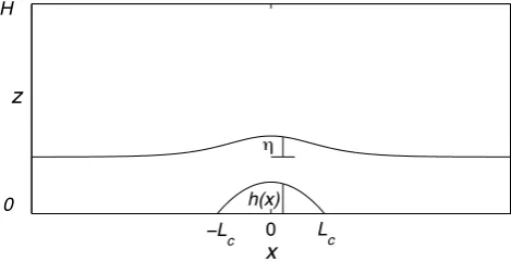
η→0 as |x| → ∞ (see Fig. 1). The boundary conditions along the flat bottom and rigid lid areη(x,0)=η(x,H )=0. In (1) the buoyancy frequencyN2= −(g/ρ0)dρ/d¯ z¯is found from the ambient density distributionρ(¯ z)¯ . The density of the fluid at any point in the flow isρ(x,z)= ¯ρ (z−η(x,z)). The wave is held stationary by a uniform oncoming flow
u=−c. Herecis the phase speed of the wave and the hor-izontal and vertical velocities in the frame of the wave are, respectively, u=c(ηz−1)andw=−cηx. The total
stream-functionψ=c(η−z).
In what follows, the variables are non-dimensionalized us-ing the depthHforxandzandpg0Hforu,w, andc. Here g0=g (ρb−ρt)/ρ0is the reduced gravity based on the den-sities at the bottom,ρb, and top,ρt, of the ambient stratifica-tion. The densities are scaled by a reference densityρ0and
N2byg0/H.
Mode-one solitary wave solutions of (1) are found for phase speedsc>c0, wherec0is the linear long-wave phase speed (found by solving (1) for∂/∂x=0 andN2=N2(z)).
0 x z
h(x) !
L
c
−L
c
H
0
Fig. 1. Sketch showing the core boundaryh(x)and the streamline displacementη. The stagnation points are atx=±Lc.
The wave amplitude increases with c until the solutions end in one of three outcomes (Lamb, 2002). One is a low Richardson number shear instability limit. If the shear limit does not occur the solutions may reach the limiting flat-top wave, or conjugate state, solution. In some cases the solu-tions reach a breaking limit defined by the presence of in-cipient overturningηz=1, oru=0 in the frame of the wave,
atz=0 (z=1) just beneath the wave crest (trough) for waves of elevation (depression). The phase speed at the point of incipient breaking is denotedc∗. A necessary condition for overturning is that the ambient stratification have finiteN2at the bottom (top) for elevation (depression) waves (cf. Lamb, 2002). In the following only waves of elevation will be con-sidered since the fluid is assumed to be Boussinesq. Waves of depression can be obtained by symmetry.
Solutions to the DJL equation can be found beyond the critical point (c>c∗) if one assumes that the function forρ(¯ z)¯ continues to increase smoothly for negative arguments (i.e., outside the physical domain). That is,N2(z−η)is defined forz¯=z−η <0 (e.g. Davis and Acrivos, 1967; Tung et al., 1982; Brown and Christie, 1998; Fructus and Grue, 2004). These solutions develop closed recirculation zones (trapped cores) within a finite region bounded by the bottom and the core boundaryh(x),|x| ≤Lc, shown schematically in Fig. 1. Because the streamlines within this core havez−η <0, they are nominally linked to streamlines that “originate” beneath the bottom and have densities outside the ambient range. This is a consequence of the violation of the assumption in (1) that all streamlines in the fluid extend tox=±∞. Fur-thermore, trapped-core solutions found by extendingN2for
One solution to this problem is to specify a uniform core density ρc≥ρb. This follows from Derzho and Grimshaw (1997) who derived a nonlinear, long-wave theory for a back-ground stratification withN≈constant and withρc=ρb. This ambient stratification is a special case since the maximum height of the trapped core, hc=h(0), remains small, per-mitting analytical progress. For more general stratifications there is no guarantee that the core height will remain small.
In this paper a model of internal solitary waves with ar-bitrary stratifications with trapped cores is developed. Once
c>c∗and a trapped core forms, the model consists of solv-ing the DJL equation outside the core and matchsolv-ing this so-lution to another model of the core structure. We will follow Derzho and Grimshaw (1997) and assume a finite core with uniform densityρc. For generality, we allowρc≥ρb, but the physically consistent choice for steady motion at long times in flows with weak diffusion is for the core density to homog-enize toρc=ρbby the Prandtl-Batchelor theorem (Batchelor, 1956; Grimshaw, 1969).
In general, the flow in an inviscid recirculating core with uniform density obeys (Batchelor, 1956)
∇2ψ=f (ψ ), (2)
wheref (ψ )is some unknown function. Frequently in prob-lems of this type, the Prandtl-Batchelor theorem is used to argue that vorticity within the closed recirculation region ho-mogenizes to the value of the vorticity of the ambient fluid on the bounding streamline (e.g., Rhines and Young, 1982). However, from (1), the vorticity of the ambient fluid flowing along the core boundary (η=h(x)),
∇2ψ=c∇2η= −N
2(0)h(x)
c ,
is not constant and the Prandtl-Batchelor argument can not be invoked. Just inside the homogeneous core, the vorticity on the bounding streamline is constant regardless of f (ψ )
sinceψis constant on a streamline. Thus the vorticity in any inviscid, uniform density core model will be discontinuous across the core boundary.
In the Derzho and Grimshaw (1997) model the core is shown to have zero vorticity (i.e. was stagnant in the frame of the wave) to leading order and the vorticity discontinuity could also be ignored. This was confirmed in subsequent nu-merical studies (Aigner et al., 1999; Aigner and Grimshaw, 2001). However, with arbitraryN2(z)and inviscid dynamics there is no similar theoretical limit on the core circulation. In principal anyf (ψ )is possible. Consideration of the forma-tion process, viscous effects and stability may constrain the possible solutions.
To make progress we will make the assumption that the core has zero vorticity. In the reference frame moving with the wave phase speedc, the core is stagnant. The full model for internal solitary waves with stagnant, uniform density
trapped cores is given in the next section where the match-ing conditions on the core boundary are given. The nu-merical procedure for finding the steady solutions is pre-sented in Sect. 3. The solitary wave solutions are explored for a particular class of ambient stratification that lead to trapped cores in Sect. 5. Because the stagnant-core assump-tion is just one of many possible choices, these new model solutions are compared to two-dimensional numerical solu-tions of the time-dependent, non-hydrostatic Euler equasolu-tions (described in Sect. 4) initiated with the new theoretical solu-tions and to solitary waves produced by a lock-release initial condition.
2 The model
As already stated, the flow in the ambient fluid outside the core is governed by the DJL equation (1) with the boundary conditions
η(x,z) →0, as|x| → ∞ η(x,1) = 0, for allx η(x,0) = 0, |x| ≥Lc
η(x,h(x)) = h(x),|x| ≤Lc.
(3)
When there is no core (c<c∗),h(x)=0 (andLc=0) so that the last condition is redundant. When a core is present, the last condition is a statement of the kinematic constraint that fluid parcels flowing alongz=0 upstream of the core must remain adjacent to the core boundary. Ifh(x)were a topo-graphic feature, rather than a internal fluid boundary requir-ing dynamical considerations, then the problem statement would be complete.
In general, inside the core (z≤h(x)for |x|≤Lc) the flow is governed by (2) with ψ=0 on the unknown boundary
z=h(x). Along the boundary the core and ambient pressures must be equal. Consider the ambient flow streamline that originates upstream at x=∞ along z=0. The dimensional Bernoulli constant on this streamline is
B=p(0)+ρ0
c2
2 , (4)
where
p(0)=
Z H
0
gρ(ξ )dξ
is the (hydrostatic) pressure atz=0 as|x|→∞. The pressure on the ambient bounding streamline is then given by
p(x,z)=p(0)−gρ(0)η+ρ0
c2
2 −ρ0 1 2
h u2b+wb2
i
. (5)
The Bernoulli function on the bounding streamline in the core is equal to the pressure at the stagnation pointx=Lc
Bc=p(Lc,0)=p(0)+ρ0
c2
2.
Thus the pressure on this bounding streamline is
pc(x,h(x))=p(0)−gρch(x)+ρ0
c2
2 −ρ0 1 2
h u2c+wc2
i . (6) The subscript c indicates core quantities anduc andwc are the core fluid velocities in the general case where the core fluid is recirculating.
The pressure must be continuous at the core boundary
z=h(x)(for|x|<Lc). Thus from (5) and (6) the matching condition is
u2b+wb2−u2c+wc2=2g(ρc−ρb) ρ0
h. (7)
This can be simplified using the kinematic boundary condi-tionw=uhxonz=h(x)for both the core and ambient flow
to give
u2b−u2c=2g(ρc−ρb) ρ0
h
1+h2
x
. (8)
When ρc=ρb, the horizontal velocity is continuous at the core boundary.
With the assumption of a stagnant core, uc=0, (8) be-comes, after using the non-dimensionalization introduced with (1),
ub=c(ηz−1)= −
2S−1−1 h 1+h2
x 1/2
, (9)
or
ηz=1− "
2(S−1−1) c2
h
1+h2
x #1/2
, z=h(x),|x|< Lc. (10)
HereS=(ρb−ρt)/(ρc−ρt)∈ [0,1]. The negative root was
chosen so thatub≤0, avoiding overturning in the free stream. Note that whenρc=ρb,S=1 and (10) giveηz=1. In this
case the velocity in the exterior flow adjacent to the core is zero (in the wave frame) and just at the overturning limit. For
ρc>ρb,ub<0 along the core.
When c0≤c≤c∗ there is no core and the DJL equation must be solved for η(x,z) subject to (3) with Lc=0. For
c>c∗the unknown core boundaryh(x)is found by solution of (1) subject to (3) along with the core condition (10). These stagnant-core solitary wave solutions should exist fromc∗up to the limiting conjugate state solutions with stagnant cores found by Lamb and Wilkie (2004) forρc=ρband White and Helfrich (2008) forρc≥ρb. The conjugate state solutions are found in a one dimensional version (∂/∂x=0) of the DJL problem, along with additional conditions that impose en-ergy and momentum flux conservation between the flows up-stream and over the uniform section of the wave. The con-jugate states have core heightshcsand speedsccs. Therefore the solitary wave solutions have core heights 0≤hc≤hcs for
c∗≤c≤ccs.
3 Stagnant-core DJL solution method
Turkington et al. (1991) developed an efficient variational technique that is frequently employed for solving the DJL equation in the absence of a core (c<c∗), or when the am-bient stratification is extended for z−η<0 (c>c∗). How-ever, this method is not easily adapted to the current problem with uniform density cores. Numerical solutions will instead be found using the Newton-Raphson technique (Press et al., 1986). In order to solve the DJL equation outside the trapped core, which is for the moment assumed to be known, (1) is re-written in a coordinate system where the physical coor-dinates(x,z)outside the core are mapped to a new coordi-nate systemσ=σ (x,z)andξ=ξ(x,z)(i.e.,x=x(ξ,σ )and
z=z(ξ,σ )). With this transformation (1) becomes
αηξξ+ βηξσ+(βησ)ξ+(γ ησ)σ
+JN
2[z(ξ,σ )−η]η
c2 =0, (11)
where
α=x2σ+z2σJ−1,
β = − xσxξ+zσzξJ−1,
γ =x2ξ+z2ξJ−1 (12)
and
J=xξzσ−xσzξ (13)
is the Jacobian of the transformation. The subscripts indi-cate partial differentiation. Here a standard boundary-fitted system
σ=z−h(x)
1−h(x), ξ=0(x), (14)
is employed. The function 0(x) is introduced to allow a stretched grid inx.
The mapped DJL equation (11) is solved in a domain 0≤σ≤1 and 0≤ξ≤1. Care is taken that L, the domain length in x, is sufficiently large to minimize effects of a finite length domain. The wave is symmetric about the crest so that ηx=hx=0 at ξ=0. From (3) and using ηx= ηξ−(1−σ )(1−h)−1hξησ, the boundary conditions become η(ξ,1)=0, η(1,σ )=0, η(ξ,0)=h(ξ ), ηξ(0,σ )=0,(15)
where it is understood thath(ξ )=0 forξ≥ξc=Lc/L. Fi-nally, in the mapped coordinate system the core pressure matching condition (10) becomes, usingηz=(1−h)−1ησ,
ησ=1−h− "
2 S−1−1 c2
(1−h)2h
1+h2ξxξ−2 #1/2
(16)
Treating the core boundaryz=h(x)as known (in each it-eration of the Newton method), (11)–(16) are approximated using second-order finite-differences. The grid has σ dis-cretized intoM+1 uniformly spaced points inσ andN+1 uniformly spaced points inξ, with aξ-grid point located at
ξc. The core boundaryhi is then defined atNc grid points where h>0. The discretized system (11)–(16) results in
(M−1)(N−1)+Nc equations for the interior values ηij
(i=2−N, j=2−M) and the Nc non-zero values of hi.
This set is solved by the Newton-Raphson method. After a Newton update, the newhi (i≤Nc) will have changed and a
new estimate of the end pointξcis found by a quadratic ex-trapolation of the last three (i=Nc−2 to Nc) core points. The solution is then interpolated onto a new grid with a grid point located at the newLc. Theξ grid is arranged such that there is approximately the same grid spacing inside and out-side the core (i.e.1ξ≈1/N everywhere). Thus the number of points,Nc, that define the core varies as the core length changes. For very small cores care is taken thatNc>3.
This solution and remapping procedure is repeated until the sum of absolute value of the variable increments and the sum of the absolute values of function residuals each drop below specified tolerances. Particular care is taken that the core lengthLcand heighthc(=h(0)) are not changing. For solutions discussed hereM=50 andN≈50L. Thus in the absence of a core the grid is approximately isotropic. In the presence of a core the grid provides sufficient resolution inx
andzto resolve the core stagnation point atLc. This solu-tion procedure is not sophisticated; however, it does produce solutions that, as will be shown below, remain essentially un-changed when used as initial conditions in time-dependent, non-hydrostatic numerical calculations. The exceptions are waves that appear to be unstable due to a physical shear in-stability.
A trapped core solution c>c∗ found using the Newton-Raphson procedure withN2(z−η)extended forz−η <0 provides an initial guesses for h(x), Lc, and the exterior
η(x,z)for the same stratification andc. Once a converged solution is obtained, it is used as the initial guess for a newc, leading to a family of solutions forc>c∗with a given ambi-ent stratification.
4 Time-dependent non-hydrostatic numerical model
The theoretical solutions obtained with the trapped-core model will be tested using numerical solutions of the invis-cid, two-dimensional non-hydrostatic equations of motion
ut+uux+wuz = −px (17)
wt+uwx+wwz = −pz−s (18)
ux+wz =0 (19)
st+usx+wsz =0. (20)
Hereuandware the horizontal and vertical velocities in the laboratory frame,s=(ρ−ρ0)/(ρb−ρt)andp is the
pres-sure (less the hydrostatic prespres-sure fromρ0). Theu,w,x, and
zhave been non-dimensionalized as (1). Pressure is scaled with ρ0g0H and time t with (H /g0)1/2. These equations are solved using the finite-volume, second-order projection method of Bell and Marcus (1992). Because of the upwind-biased Godunov evaluation of the nonlinear terms the method is stable, requires no explicit dissipation, and introduces sig-nicant numerical dissipation only when large gradients oc-cur on the grid scale. The numerical method has been used successfully for studies of large-amplitude internal solitary waves (e.g., Lamb, 2002; White and Helfrich, 2008), and tests of the code show that large internal solitary waves with-out trapped cores propagate distances of more than 100H
with the correct phase speed, amplitude, shape, and minimal loss of energy (<1%).
Two types of calculations are considered. In the first, the stagnant-core DJL solitary waves are tested by using these steady solutions as initial conditions. In the second, trapped-core waves are generated by a lock-release initial condition
ρ(x,z,t=0)=
¯
ρ(z),¯ x≥Ld
¯
ρ(z¯−hd), x<Ld and z¯≥hd
ρd, x<Ld and z<h¯ d
(21)
The region of fluid held behind the lock extends fromx=0 tox=Ld. Herehdis the depth of a lower uniform-density layer,ρd≥ρb, beneath the ambient stratification. This initial condition mimics the experiments of Grue et al. (2000) and Carr et al. (2008). In both cases the solutions use uniform grids with vertical grid cell size of 1z=1/150. The hor-izontal resolution1x=0.01 in the DJL model initial con-dition cases and1x=0.01−0.02 for the lock-release runs. The time-stepping is controlled internally to keep maximum Courant number less than 0.625. The DJL solution initial condition runs use no normal flow boundary conditions inz
and inflow/outflow boundary conditions inx. A uniform flow
u= −cwiths= ¯s(z)¯ is imposed at the right boundary with an open boundary at the left. The waves are traveling in the positive-xdirection in the laboratory frame. The lock-release runs have no normal flow conditions on all boundaries.
5 Results
To illustrate the solutions to the DJL model for large-amplitude waves a background density given by
¯
ρ(z)¯ =1+(ρb−ρt) ρ0
¯
s(z),¯ (22)
with ¯
s(z)¯ =1−tanh(λz)¯
tanhλ (23)
z t = 0
−2 −1.5 −1 −0.5 0 0.5 1 1.5 2
0 0.2 0.4
z t = 30
−2 −1.5 −1 −0.5 0 0.5 1 1.5 2
0 0.2 0.4
z t = 70
−2 −1.5 −1 −0.5 0 0.5 1 1.5 2
0 0.2 0.4
z t = 200
x − ct
−2 −1.5 −1 −0.5 0 0.5 1 1.5 2
0 0.2 0.4
Fig. 2. Evolution of an extended-s¯ DJL solution forλ=8 andc=
0.4. Contours ofsin intervals of 0.1 fors≤1 (outside the core) and 0.025 fors>1 (inside the core) are plotted. Times are indicated in the panels. Note that only part of the domain is shown.
5.1 Extended-¯sDJL waves
We first examine waves obtained by extending the ambient
N2(z)¯ for z <¯ 0 and call those solutions “extended-s¯ DJL” waves. The time-dependent evolution of an extended-s¯DJL wave forλ=8 andc=0.4 is shown in Fig. 2. Figure 3 shows a larger wave withc=0.58 and the sameλ=8. The top panel of each figure shows the theoretical solutions with recirculating (negative vorticity) cores with densities greater than the am-bient density along the bottom,s(¯ 0)=1 and statically unsta-ble core density distributions. The amplitudeηM, core height
hcand core lengthLcof these extended-s¯DJL solutions for
λ=8 and 4 are shown by the dashed lines in Fig. 8. The wave amplitude ηM is defined as the maximum streamline displacement of the flow outside the core at the wave crest. Forλ=8 (4), the linear long-wave phase speed c0=0.226 (0.285), the critical overturning speed c∗=0.331 (0.383) and the extended-s¯ DJL conjugate state speed ccs=0.582 (0.505).
The Richardson number, Ri, of each of these waves falls between 0 and 0.25 in a region in the upper, stably-stratified portion of the core that extends in thinning bands to the two stagnation points as shown in Fig. 4. Recent work by Carr et al. (2008), Fructus et al. (2009), and Barad and Fringer (2010) has shown that internal solitary waves are unstable to Kelvin-Helmholtz instability when the minimum Richard-son number is less than about 0.1 and the ratiolRi/ lW≥0.86.
z
t = 0−5 0 5
0 0.5 1
z
t = 7.5−5 0 5
0 0.5 1
z
t = 10−5 0 5
0 0.5 1
z
t = 30−5 0 5
0 0.5 1
z
t = 100−5 0 5
0 0.5 1
z
t = 200x
−
ct
−5 0 5
0 0.5 1
Fig. 3. Evolution of an extended-s¯DJL solution forλ=8 andc=
0.58. Contours ofsin intervals of 0.1 are plotted.
x z
(a)
−00.5 0 0.5
0.1 0.2
x z
(b)
−2 −1.5 −1 −0.5 0 0.5 1 1.5 2
0 0.2 0.4 0.6
HerelRiis the horizontal length of the Ri≤0.25 region andlW is the solitary wave width (twice the distance from the crest to where η of the maximum amplitude streamline equals 0.5ηM). The latter condition is related to the time (or dis-tance) required for the unstable waves to grow before they are swept out of the unstable region and left behind the soli-tary wave. However, the extended-s¯waves are different from the situations considered in Fructus et al. (2009) and Barad and Fringer (2010) in two important ways. The low Ri region is confined to the recirculating core where disturbances could re-enter the unstable region. Furthermore, streamlines in the low Ri region also pass through the gravitationally unstable lower core.
In the time-dependent solution for the c=0.4 wave in Fig. 2 the trapped core does become unstable. The instability first appears as a wobble, or distortion, of the core center as shown att=30. Byt=70 the core begins to breakdown and density inversions are evident. Betweent=70 andt=200 the flow stabilizes to a new trapped core wave with wave am-plitudeηM=0.208 and speedc=0.394 that are only slightly different from the original wave. However, the trapped core is smaller and the maximum core density has decreased from
s=1.192 to 1.092 and become more homogeneous. The ori-gins of the instability are not clear in this case. The initial wobble could be the result of either gravitational or shear in-stability.
The instability and its consequences are much more dra-matic for the larger,c=0.58, wave in Fig. 3. This exam-ple also provides a clearer indication of the processes in-volved. Att=7.5 the first disturbances have developed in the lower, gravitationally unstable part of the core. These disturbances grow and are swept up into the upper half of the core near the forward stagnation point. They then appear to excite Kelvin-Helmholtz billows near the wave crest in the low Ri band (t=10). An analysis of the energetics of the disturbances at small times would be informative but is be-yond the current scope of this work which is focussed on the stable core states. Byt=30 the instability has nearly de-stroyed the wave. Amazingly, betweent=50 and 100 a new trapped-core solitary wave forms from the disorganized flow. Betweent=100 and 200 the flow completely stabilizes to a slower wave withc=0.558.
Figure 5 shows a comparison of the vertical profiles of
u−c, s, and Ri at the crests of the initial (t=0) and the equilibrated (t=200) waves. The final core has a nearly ho-mogeneous density core,s≈1.18, that is much less than the maximum value ofs=1.829 att=0. The horizontal veloc-ity along the bottom is larger than the initial wave, indicat-ing an increase in the magnitude of the core vorticity. The wave is stable even though Ri<0.25 in the upper part of the core (0.38< z <0.58). This unstable region extends to the two stagnation points similar to the unstable band att=0 in Fig. 4b. But unlike the initial wave, the uniform density of the final core inhibits the gravitational instability. It appears that shear instabilities are unable to grow sufficiently without
−2 0 2
0 0.2 0.4 0.6 0.8 1
u−c z
(a)
0 1 2
0 0.2 0.4 0.6 0.8 1
s (b)
0 0.5
0 0.2 0.4 0.6 0.8 1
Ri (c)
Fig. 5. The vertical profiles of (a)u−c, (b)s, and (c) Ri through the center of the solitary waves att=0 (solid) andt=200 (dashed) in Fig. 3.
0 0.05 0.1 0.15 0.2
−12 −10 −8 −6 −4 −2 0
! "2!
Fig. 6. Scatterplot (black) of the core vorticity versus streamfunc-tion att=200 for the case in Fig. 3. The light gray region indicates the values of streamfunction and vorticity in the core att=0.
coupling with the gravitational instability. The low Ri region nearz=0.9 is a result of the vanishing stratification there and remained stable in the calculation.
The final core vorticity is the same sign as the initial core and ambient vorticities. A scatter plot of vorticity versus streamfunction within the core is shown in Fig. 6. A clear relationship,∇2ψ=f (ψ ), has developed in the core. It is distinct from the broad range of core vorticity and stream-function values att=0 (the light gray area in Fig. 6). The increase in the magnitude of the core vorticity following the instability and equilibration is clear from this figure. A sim-ilar, although different, relationship develops for the smaller wave in Fig. 2.
x
−
ct
z
−03 −2 −1 0 1 2 3
0.1 0.2 0.3 0.4 0.5
Fig. 7. Stagnant-core DJL solution forλ= 8,sc=1, andc=0.4. The core is indicated by the shading and the thin lines arescontours in increments of 0.1. The area inside the heavy line and above the core has Ri≤0.25. Note that only the lower half of the water column is shown.
homogeneous density cores with distinct relationships be-tween core vorticity and streamfunction. Both of these out-comes support the theoretical model introduced in Sect. 2. However, the current restriction of the theoretical model to stagnant-core solutions is a clear limitation. Regardless, it is useful to explore the stagnant core solution properties, in-cluding stability, and ask if this model provides reasonable estimates of trapped-core waves that develop from a general initial-value problem such as a lock-release.
5.2 Stagnant-core DJL waves
An example of a stagnant-core solution forλ=8,sc=1, and
c=0.4 is shown in Fig. 7. This wave has the same ambi-ent stratification and phase speed as the extended-s¯wave in Fig. 2. It has slightly larger amplitude, smaller core height, and larger core length than the extended-s¯ wave. Another difference is that the stagnant-core wave has a region of Ri<0.25 above the core (bounded by the heavy line in Fig. 7). The minimum Ri=0.154 andlRi/ lW=0.37. Recall that the extended-s¯examples above had the region of low Richardson numbers located entirely within the core (with the exception of low values in the the very weakly stratified region near the upper boundary; cf. Fig. 5).
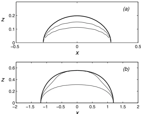
Figure 8 summarizes the properties of the stagnant-core DJL solutions. The wave amplitude,ηM, core heighthc, and core lengthLc are shown as functions ofcforλ=4 and 8. For comparison, the extended-s¯DJL wave properties are also plotted. For both values ofλ, the stagnant-core solutions be-gin at the incipient overturning wave speedc∗and end before reaching the limiting conjugate state solutions (open circles) atc=0.446 and 0.468 forλ=4 and 8, respectively. It was not possible to continue the solutions beyond what is shown in the figure. The reason for the failure of the numerical solu-tion procedure is unclear, although the likely candidate is the emergence of the regions of low Ri. Similar numerical diffi-culties have been encountered by Lamb (2002) when solving for solitary waves in nearly two-layered stratifications using
0.2 0.3 0.4 0.5 0.6
0 0.2 0.4 0.6 (a)
!M
0.2 0.3 0.4 0.5 0.6
0 0.2 0.4 0.6 (b)
hc
0.2 0.3 0.4 0.5 0.6
0 0.5
1 (c)
c Lc
0.3 0.35 0.4 0.45 0.5 0
0.2 0.4 0.6 0.8
(d) !M
0.3 0.35 0.4 0.45 0.5 0
0.2 0.4 0.6 0.8
(e) h
c
0.3 0.35 0.4 0.45 0.5 0
0.5 1 1.5 (f)
c L
c
Fig. 8. The wave amplitudeηM, core heighthc, and core lengthLc vs. wave speedcfrom the stagnant-core DJL solutions are shown by the solid lines forsc=1 andλ=8, (a)–(c), andλ=4, (d)–(e). The open circles indicate the conjugate state solutions. The dashed lined and open squares show the same quantities from the
extended-¯
t = 0
z
−3 −2 −1 0 1 2 3
0 0.5
t = 20
z
−3 −2 −1 0 1 2 3
0 0.5
t = 50
z
−3 −2 −1 0 1 2 3
0 0.5
t = 100
x
−
ct
z
−3 −2 −1 0 1 2 3
0 0.5
Fig. 9. Evolution of a stagnant-core DJL solution forλ=8,sc=1, andc=0.4. The panels show contours ofsat the times indicated. The contour intervals are 0.1 fors≤0.9 and 0.025 fors >0.9. Note that only the lower half of the domain is shown.
the Turkington et al. (1991) solution method. Forλ=8 (4) the Richardson number first drops below 0.25 atc=0.368 (0.395) and by the last solution found the minimum Ri above the crest is 0.073 (0.115) and the ratiolRi/ lW=0.8 (0.38).
From Fructus et al. (2009) and Barad and Fringer (2010), these waves should be stable to shear instability. Figure 9 shows the time-dependent evolution of the stagnant-core DJL wave in Fig. 7 (λ=8 and c=0.4). In this case, the ini-tial stagnant-core wave is subject to an instability that orig-inates along the core boundary in the low Ri zone. The Kelvin-Helmholtz billows are clear att=20. The instabil-ity is rather mild and betweent=50 and 100 the flow re-stabilizes to a wave that is only slightly different from the ini-tial wave. Figure 10a–d shows the wave properties (s,u−c,
w, and vorticity∇2ψ) from the numerical solution averaged betweent=90 and 100. The core density is slightly inho-mogeneous. The instability has injected ambient fluid into the core and baroclinic vorticity production and advection produces a weak positive vorticity (the initial and ambient vorticity is everywhere negative) (see Fig. 10d). The flow in the core is very weak (see Fig. 10b and c), but does include a band ofu−c >0 located above the bottom. In contrast, in the extended-s¯solutions the region ofu−c >0 lies along the bottom (i.e. core vorticity is negative). The phase speed of the equilibrated wavec=0.399 is nearly the same as the stagnant-core model wave. The core boundary from the ini-tial wave (heavy solid line in Fig. 10a–c) also agrees with
(a) s z
−01.5 −1 −0.5 0 0.5 1 1.5 0.5
−01.5 −1 −0.5 0 0.5 1 1.5 0.5
(b) u − c z
−01.5 −1 −0.5 0 0.5 1 1.5 0.5
(c) w z
−01.5 −1 −0.5 0 0.5 1 1.5 0.5
(d) !2"
x − ct z
−0.6 −0.4 −0.2 0 0.2 0.4 0.6 0.8 1 0
0.2 0.4 0.6 0.8 1
z
u − c s
(e)
Fig. 10. Averages overt=90−100 for the run in Fig. 9. (a)s, (b)
u−c, (c)w, (d)∇2ψ. Thescontour interval is 0.1 fors≤0.9 and 0.025 fors >0.9. The contour interval is 0.03, 0.015, and 0.5 for (b)–(d), respectively, with solid lines for values≥0. (e) Vertical profiles ofu−c and s atx−ct=0 from the theory (solid) and numerical model (dashed). The heavy solid line in (a)–(d) shows the core boundary from stagnant-core DJL solution.
the apparent core shape in the equilibrated wave. In particu-lar, the region of near-zero vertical velocities in Fig. 10c lies entirely with the initial core boundary.
(a) t = 0
z
−30 −2 −1 0 1 2 3
0.5
(b) t = 20
z
−30 −2 −1 0 1 2 3
0.5
(c) t = 40
z
−30 −2 −1 0 1 2 3
0.5
(d) t = 100
x − ct z
−30 −2 −1 0 1 2 3
0.5
−0.5 0 0.5 1
0 0.2 0.4 0.6 0.8 1
z
u − c s
(e)
Fig. 11. Evolution of a stagnant-core DJL solution forλ=8,sc=
1.1, andc=0.4. (a)–(d) Contours ofs are shown in at the times indicated. The contour intervals are 0.1 fors≤0.9 and 0.025 for
s >0.9. Note that only the lower half of the domain is shown. (e) Comparison ofu−candsat the wave crest att=100 (dashed) with the stagnant-core DJL solution withλ=8, sc=1 andc=0.394 (solid).
should equilibrate tos=0.973, the value of the density flow-ing along the boundflow-ing streamline. The transport of ambient fluid into the core and the expelling of core fluid out the back of the wave is an example of Lagrangian advection across a hyperbolic trajectory (Wiggins, 2005). The shear instability along the core boundary provides the time-dependent forc-ing of the hyperbolic trajectory (the boundforc-ing streamline ap-proaching the rear stagnation point), subsequent lobe forma-tion and transport.
The equilibrated wave has a region of Ri<0.25 just above the core with minimum Ri≈0.15 andlRi/ lW≈0.37, nearly
identical to the initial wave. This suggests that the instability observed in the numerical solution could be a consequence of the initial vorticity discontinuity at the core boundary. One effect of the instability is to eliminate the vorticity disconti-nuity and reduce the vertical shear at the core boundary (see Fig. 10d).
Another example of the evolution of a stagnant-core DJL wave is shown in Fig. 11. As in the previous exampleλ=8 and c=0.4, but the core of the initial wave has density
sc=1.1. Recall from the boundary condition (8) that the
jump in density across the core boundary gives a jump in ve-locity, which should enhance the likelihood of shear instabil-ity. The time-dependent solutions show that large overturns develop at the core boundary byt=20. However, byt=40 the instability has weakened considerably and byt=100 the wave has stabilized. This final wave propagates at a speed
c=0.394 and has a core that is nearly stagnant and homoge-neous as shown by the dashed lines in Fig. 11e. The mixing from the instability has again replaced the initial core fluid withs=0.97 fluid. Thus the new wave is close to a stagnant-core DJL wave withsc=1. The solid lines in Fig. 11e show the vertical profiles ofu−candsfrom the stagnant-core DJL solution withc=0.394. With the exception of the weak core circulation and the slightly lower density of the core fluid, the equilibrated wave agrees very well with the theory.
Time-dependent numerical solutions initialized with stagnant-core DJL waves withsc=1 and other values ofc
for bothλ=4 and 8 show similar behavior. An initial pe-riod of shear instability is followed by flow stabilization to a large-amplitude wave with properties very close to those predicted by the stagnant-core DJL model. The amplitude
ηM, core heighthc, and core lengthLcof these equilibrated waves for λ=4 and 8 are shown in Fig. 12 (by the open circles). The equilibrated wave from Fig. 11 is indicated by the open diamonds in Fig. 12a–c. The valueshcandLcare determined from the vertical and horizontal extent of the re-gion of near-zero vertical velocities (i.e. thew=0 contours) as shown in Fig. 10c. There is some uncertainty in choosing these values that is reflected in the slight scatter of the data. However, the agreement between the stagnant-core DJL the-ory and the numerical results is quite good.
These results support the stagnant-core theory despite the fact that the full numerical solutions produce cores with weak circulation with positive vorticity and nearly homogeneous density. However, this is not too strict a test of the theory as it says that if flow starts close enough to the stagnant-core solution, it will remain near it. The calculations shown in Figs. 2 and 3, on the other hand, show that solutions with nearly homogeneous density, but vastly different core circu-lation are possible. In those cases the wave propertiesηM,
hc, andLc do not agree with the stagnant-core model (not shown).
0.250 0.3 0.35 0.4 0.45 0.5 0.1
0.2 0.3 0.4 !M (a)
0.250 0.3 0.35 0.4 0.45 0.5 0.1
0.2 0.3 0.4 h
c (b)
0.250 0.3 0.35 0.4 0.45 0.5 0.2
0.4 0.6 0.8
c L
c (c)
0.350 0.4 0.45
0.1 0.2 0.3 0.4
!M
(d)
0.350 0.4 0.45
0.1 0.2 0.3 0.4
h c
(e)
0.350 0.4 0.45
0.2 0.4 0.6
c L
c
(f)
Fig. 12. Comparison of wave amplitudeηM, core heighthc, and core lengthLcversus wave speedcfrom the stagnant-core DJL lutions (solid lines), numerical solutions initiated with the model so-lutions (open circles), and from the lock-release runs (open squares) forλ=8, (a)–(c), andλ=4, (d)–(f). The solid circles show the the-oretical conjugate state limits. The open diamonds in (a)–(c) show the equilibrated wave initiated with a stagnant-core DJL solution withsc=1.1 and the open triangles show the conjugate state prop-erties from a lock-release numerical run from White and Helfrich (2008).
t = 0
z
0 2 4 6 8 10 12 14 16 18
0 0.5 1
t = 10
z
0 2 4 6 8 10 12 14 16 18
0 0.5
t = 20
z
0 2 4 6 8 10 12 14 16 18
0 0.5
t = 30
x z
0 2 4 6 8 10 12 14 16 18
0 0.5
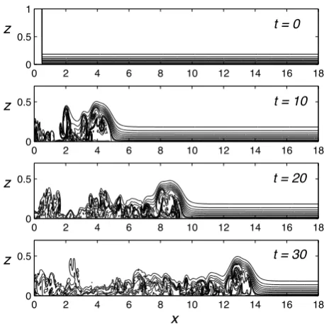
Fig. 13. Lock-release run forλ=8,hd=1,Ld=0.6 andsd=1. Contours ofsare shown at the indicated times. The contour interval is 0.1 fors≤0.9 and 0.025 fors >0.9. Note that part of vertical domain is shown fort >0.
A close-up of the wave at t=300 is shown in Fig. 14. This long-time evolution is found by taking the leading wave from the lock-release run att=30 as the initial condition for a run with inflow-outflow boundary conditions with a uniform inflow velocity magnitude equal to the propagation speedc=0.435 from the lock-release run. The wave contin-ues to adjust until aboutt=180 after which the phase speed,
c=0.417, is constant. This final wave has a well-defined core region from thew=0 contour (Fig. 14c). There is a re-circulation cell shown by the streamfunction in Fig. 14d and the horizontal velocitiesu−c >0 (Fig. 14b). However, the recirculation cell (with positive vorticity) sits above the bot-tom. Streamlines from the ambient flow ahead of the wave split to flow around this recirculation cell. This is an instan-taneous picture of the flow. The flow over the core is still weakly unstable (see the cat’s eye of the Kelvin-Helmholtz billows on the trailing side of the wave), inducing a slow, continuous transport of ambient fluid into the core, and ex-pelling core fluid out the back of the wave. This results in a nearly uniform density in the recirculation cell ofs≈0.88. The densest ambient fluid flows beneath this cell and is less involved in the cross-boundary transport than the (less dense) ambient streamlines that pass over the cell.
(a) s
z
−03 −2 −1 0 1 2 3
0.5
−03 −2 −1 0 1 2 3
0.5
(b) u − c
z
−3 −2 −1 0 1 2 3
0 0.5
(c) w
z
x−ct
z (d) !
−01.5 −1 −0.5 0 0.5 1 1.5
0.2
−0.6 −0.4 −0.2 0 0.2 0.4 0.6 0.8 1 0
0.2 0.4 0.6 0.8 1
z
u − c s
(e)
Fig. 14. The leading solitary wave from Fig. 13 att=300. (a)s, (b)u−c(c)wand (d)ψ. The wave travels at a constant speed
c=0.417 fort >100. Thescontour interval is 0.1 fors≤0.9 and 0.025 fors >0.9. The contour interval is 0.05 in (b) and 0.02 in (c), with solid lines for values≥0. Theψ contour intervals in (d) are 0.001 forψ≥0.01 and 0.04 otherwise. (e) Vertical profiles ofu−c
ands atx−ct=0 from the theory (solid) and numerical model (dashed). Note that the horizontal and vertical scales in (d) differ from those in (a)-(c).
slope-shelf topography (Lamb, 2002). Figure 14e shows the vertical profiles ofu−cands atx−ct=0 from the wave att=300 and the stagnant-core theory prediction for a wave withc=0.409 and λ=8. The agreement above the core (z >0.2) is very good.
From theu−cprofile it can be seen that the vorticity in the core is positive and opposite sign from the vorticity in the ambient fluid. This positive vorticity is not a direct prod-uct of the initial adjustment immediately following the lock-release. Rather, it is a product of vorticity produced in the unstable shear flow surrounding the core. Figure 15 shows a close-up of the vorticity structure att=10 from Fig. 13. At this time the vorticity within the developing core is nearly zero. Patches of positive vorticity from baroclinic
produc-x z
!2"
0 1 2 3 4 5 6
0.6
0.5
0.4
0.3
0.2
0.1
0
−5 0 5
Fig. 15. The vorticity structure of the leading wave att=10 from the lock-release numerical run in Fig. .
−−0.0126 −0.01 −0.008 −0.006 −0.004 −0.002 0 −4
−2 0 2 4 6
!
"
2!
Fig. 16. Scatterplot of the core vorticity versus streamfunction for the wave in Fig. 14.
tion are present in the unstable flow around the core. Over time, some of this positive vorticity fluid is entrained into the core. In general, the lock-release runs lead to cores with larger magnitude positive vorticity than the stagnant-core ini-tial conditions. This appears to be a consequence of an iniini-tial wave that is more unstable to shear instability along the core boundary, and hence greater baroclinic vorticity production and subsequent entrainment of this vorticity into the evolving core.
A scatterplot of vorticity versus streamfunction from within the core is shown in Fig. 16. For this plot the core region is defined to lie below the arc fromx−ct= ±0.48 through the center of the chain of cat’s-eye vortices (which corresponds closely to the core defined byw=0 in Fig. 14c). Within the closed recirculation cell where ψ≤ −0.005, a clear streamfunction-vorticity relation has emerged with the positive vorticity values clustering along a linear trend with
ψ.
respectively, the amplitudes and speeds of these waves agree quite well with the stagnant-core theory. Furthermore, ifhc andLc are defined by thew=0 contours (see above) the agreement with the theory is also good. If the fluid behind the dam has densitysd>1, the solitary wave that emerges will, after enough time, expel the dense fluid and have a leaky core with densitys≤1. Despite the significant dif-ferences between the waves produced via a lock-release and the stagnant-core DJL theory, the theory does a surprisingly good job of capturing the overall wave properties.
The lock-release runs produced solitary waves that forλ= 8 were always slower and smaller than the fastest stagnant-core DJL wave found and forλ=4 were only slightly faster than the maximum theoretical solution. This was the case despite initial conditions that have a larger volume of fluid of densityρbbehind the dam than the core volume of the largest wave. The available potential energy of the initial state is also greater than the total energy of the largest theoretical solitary wave. White and Helfrich (2008) did find conjugate state solutions (indicated by the open triangles) from lock-release runs withLd1 andhd→1 when the initial available po-tential energy per unit length of the region behind the dam was greater than the total energy per unit length of the (in-finitely long) conjugate state. The leading face of the conju-gate state waves were smooth, but intense Kelvin-Helmholtz billows formed on the uniform region of the conjugate state wave crest (see Fig. 17b in White and Helfrich, 2008).
The wave produced in the lock-release example in Fig. 13 appears to be more unstable than the waves in the laboratory experiments of Grue et al. (2000) and Carr et al. (2008). One possible reason for this difference is that initial dam height
hd=1, which is the maximum possible, is larger than the lab-oratory experiments (Grue et al., 2000 usedhd≈0.5 in ex-periments that produced large trapped-core waves). Thus the initial state in the model has more available potential energy. The stratification is also different. In the laboratory exper-iments an equivalentλ≈6. Lastly, the two-dimensionality of the numerical model prohibits the transverse breakdown of the Kelvin-Helmholtz billows. Detailed wave properties will depend on whether the third dimension is included, es-pecially if a careful comparison is to be made with the exper-iments. However, the calculations still provide insight into wave development and a systematic test of the theory.
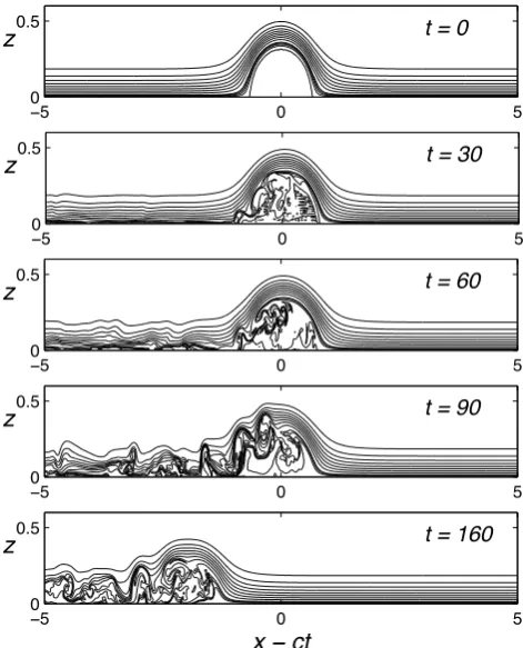
One last example of wave evolution is shown in Fig. 17 for a case initiated with the largest stagnant-core wave found withλ=8 andsc=1 atc=0.45 . As in the earlier exam-ples the wave is initially unstable to shear instability local-ized along the core boundary. Unlike the previous exam-ples, the instability does not weaken. Rather, the instability strengthens betweent=60 and 90 such that the wave con-tinually diminishes in size and speed untilt=200 when the wave reached the downstream end of the domain and the cal-culation was stopped. If the domain were longer, the flow might eventually equilibrate to a new wave as in the ear-lier examples, but any final wave will be very much smaller
t = 0
z
−5 0 5
0 0.5
t = 30
z
−5 0 5
0 0.5
t = 60
z
−5 0 5
0 0.5
t = 90
z
−5 0 5
0 0.5
t = 160
x
−
ct
z
−5 0 5
0 0.5
Fig. 17. Evolution of the largest stagnant-core DJL solution found forλ=8 andsc=1 atc=0.45. Contours ofsare shown at intervals of 0.1 fors≤0.9 and 0.025 fors >0.9. Note that only the lower portion of the domain is shown.
than the initial wave. Recall that the initial wave has a min-imum Richardson number above the core of 0.073 and that
lRi/ lW=0.8. These values put the wave closer to the insta-bility boundary found by Fructus et al. (2009) and Barad and Fringer (2010). It is also consistent with the suggestion that the failure to find stagnant-core DJL solutions forc >0.45 is related to flow instability and helps explain why the lock-release runs produced solitary waves within the range of stagnant-core solutions.
6 Conclusions
inviscid theory. For simplicity, and to make progress, we have chosen the simplest possible core flow – a stagnant flow in the steady frame of the wave. This homogeneous density, stagnant-core DJL model connects the incipient overturning solitary wave to the limiting amplitude stagnant-core conju-gate state solutions of Lamb and Wilkie (2004) and White and Helfrich (2008).
Solutions for steady, stagnant-core DJL internal solitary waves were obtained numerically and properties of the waves were compared to those found by extending the ambient stratification,s(z¯ −η)for negative arguments. For the strati-fications considered, differences in the resulting wave prop-erties could be substantial, especially as the wave amplitude increases. We note though, that if the ambient stratification is extended differently, then the disagreement can be reduced. For example, ifs¯is extended with
¯
s(z)¯ =1− N 2 0z¯ 1−N02(sc−1)−1z¯
, forz¯≤0, (24)
whereN02= − ¯sz(¯ 0) from the ambient stratification. This extension gives continuous density and N2 at z¯=0, and avoids numerical problems associated with discontinuousN2
in the usual DJL solution methods. It asymptotes tosc for
¯
z→ −∞, and forsc−11, the core density will be nearly
homogeneous with maximum density only slightly greater than the ambient environment and the recirculation will be weak. Wave properties computed withsc=1.02 are nearly the same as the stagnant-core properties shown in Fig. 8. The solution branches even stop at nearly the same wave speed. This extension procedure, though not the form fors¯above, has been previously proposed by Brown and Christie (1998). While these special extended-s¯ solutions are only slightly different from the new stagnant-core model, the latter pro-vides a theoretical framework for developing homogeneous core solutions with specified circulation.
Time-dependent numerical solutions of the Euler equa-tions initiated with the stagnant-core DJL soluequa-tions agree well with the theory, though the solutions exhibit shear in-stability along the core boundary and develop a weak recir-culation (of opposite sign vorticity) within the core. The time-dependent solutions indicate that low Ri regions near the wave crest lead to wave instability that appear to explain the limited range of achievable wave amplitudes.
During the final stages of the submission process this pa-per, the authors were made aware of a recently submitted manuscript by King et al. (2010) that described a new nu-merical method for solving the DJL equation. They were able to compute waves with stagnant, uniform density cores using an extension of the ambient density structure similar to (24), but with much more rapid transition than above. Two-dimensional, time-dependent numerical calculations initi-ated with both a stagnant-core wave and a wave found by extending the ambient density profile, were qualitatively sim-ilar to the results in this paper.
Solitary waves produced from a lock-release also agree reasonably with the stagnant-core model for wave amplitude, core height and core length. However, the core heights and lengths used in the comparison are defined, somewhat arbi-trarily, from the vertical velocity fields. There is a recircu-lating core, but it has vorticity of opposite sign from the am-bient flow and is off the boundary. Furthermore, the cores are not isolated from the ambient flow. Unsteadiness from shear instability gives rise to fluid transport into and out of the nominal core region such that the core density is less than the densest ambient fluid. As in the stagnant-core initi-ated runs, the positive vorticity in the core must be the result of baroclinic vorticity production as the ambient vorticity is negative.
Very different core circulations from those described above can occur, as illustrated by Figs. 3 and 6. In this ex-ample, the core is nearly homogeneous and has vorticity of the same sign as the initial condition, but with very a dif-ferent vorticity-streamfunction relation. This emphasizes the role of transient wave formation, instability and dissipative processes on the final core structure and circulation. It also raises the question of whether there are general principles that place limits on the range of realizable core flows. Cer-tainly, the presence of shear instability and the tendency of the flow to adjust to marginal stability is one such limit. This is an avenue for future investigation.
As mentioned in the Introduction, Grue et al. (2000) and Carr et al. (2008) carried out experiments on internal solitary waves produced from a lock-exchange and found that large waves could have regions of u > c. We have not made a detailed comparison with their experiments. There are, how-ever, several aspects of the experiments that are in qualitative agreement with the results presented here. One is that in ex-periments with apparent trapped cores, the vertical profiles of horizontal velocity at the wave trough (the experiments pro-duced waves of depression) show thatu/c≈1 in the upper water column as shown in Figs. 14, 15, and 18 in Grue et al. (2000) and Figs. 9 and 20 in Carr et al. (2008). It is not clear that this depth range represents the full height of a core since the authors do not provide independent estimates of the core height (e.g. from the density fields). However, the height of this zone at the wave center is approximately equal to the depth of the upper, linearly stratified layer (hupper≈0.2H). The wave amplitudes, measured by the vertical displacement of the interface between the two layers, are also approxi-mately equal to the upper layer depth. From Fig. 7 it is clear that the height of the core is always less than the wave ampli-tude (defined somewhat differently in the theory), except for the largest waves where they are approximately equal. Thus the experimental core heights defined by theu≈cdepth are at least qualitatively similar to the theory. Of course, the stratifications are different and this should be taken into ac-count in any detailed comparison, but this is suggestive that
Another important feature of the experiments is that the cores are not completely stagnant. Small turbulent vortices are present both within the core and along the core boundary (e.g., Fig. 20 in Grue et al., 2000). And there is evidence of small, but finite, vertical shear in the cores. As the free surface is approached from below, the fluid velocity declines, producing a zone of vorticity within the core with opposite sign from the open portion of the flow (see Fig. 20 in Carr et al., 2008, although this may be an artifact of the no-slip lid in this particular experimental run). So while not conclusive, these experiments do lend support to the stagnant-core theory and numerical modeling results.
Grue et al. (2000) also report that instability limited the maximum observed wave amplitude to be less than for the theoretical maximum wave (found using an extended-s¯DJL model). The conclusion that the stagnant-core waves are lim-ited by instability is in qualitative agreement with these ex-periments. We note that in the experiments done by Carr et al. (2008) the fluid behind the lock was not seeded with particles (for PIV), yet the core regions in their Figs. 2–7 are filled with particles (M. Carr, personal communication, 2010), indicating that ambient fluid is incorporated into the core. Unfortunately, neither study made direct measurements of the densities within the core region and these, along with experimental measurements of the trapped-core properties over a broad range of parameters, would be valuable.
Mass transport by large-amplitude internal solitary waves is thought to play an important role in cross-shore larvae transport (Pineda, 1999; Helfrich and Pineda, 2003). If the wave amplitude is large enough for trapped-core formation, the question of core structure and leakiness will be important. The streamline pattern in Fig. 14d implies that larvae near the free surface (for waves of depression) may not be incor-porated into the core, while larvae residing slightly below the free surface could be brought into the a leaky core for a finite period of time and experience significant horizontal trans-port during that period at the wave phase speed. Similar con-cerns exist for possible transport of fine suspended sediment by waves of elevation propagating along the sea floor. The trapped-core waves observed by Klymak and Moum (2003) show evidence of both acoustic backscatter from biological activity and optical backscatter from fine sediments.
Finally, the time-dependent numerical calculations pre-sented here are all two-dimensional. Clearly, the three-dimensional evolution of the solutions needs to be explored. The effects of the gravitational and Kelvin-Helmholtz insta-bilities on the wave evolution and mixing will certainly be different in three dimensions, possibly leading to different core states. Fluid exchanges between the core and the am-bient will likely be modified from the two-dimensional runs. Also, waves with recirculating (or stagnant) cores may them-selves be unstable to transverse perturbations.
Acknowledgements. This work is supported as part of the Office of Naval Research NLIWI and IWISE program grants N00014-06-1-0798 and N00014-09-1-0227.
Edited by: R. Grimshaw
Reviewed by: K. Lamb and another anonymous referee
References
Aigner, A. and Grimshaw, R.: Numerical simulations of the flow of a continuously stratified fluid, incorporating inertial effects, Fluid Dyn. Res., 28, 323–347, 2001.
Aigner, A., Broutman, D., and Grimshaw, R.: Numerical simula-tions of internal solitary waves with vortex cores, Fluid Dyn. Res., 25, 315–333, 1999.
Akylas, T. and Grimshaw, R.: Solitary internal waves with oscilla-tory tails, J. Fluid Mech., 242, 279–298, 1992.
Barad, M. F. and Fringer, O. B.: Simulations of shear instabilities in interfacial gravity waves, J. Fluid Mech., 644, 61–95, 2010. Batchelor, G. K.: On Steady laminar flow with closed streamlines
at large Reynolds numbers, J. Fluid Mech., 1, 177–190, 1956. Bell, J. B. and Marcus, D. L.: A second-order projection method
for variable-density flows, J. Comp. Phys., 101, 334–348, 1992. Brown, D. J. and Christie, D. R.: Fully nonlinear solitary waves in
continuously stratified incompressible Boussinesq fluids, Phys. Fluids, 10, 2569–2586, 1998.
Carr, M., Fructus, D., Grue, J., Jensen, A., and Davies, P. A.: Convectively induced shear instability in large am-plitude internal solitary waves, Phys. Fluids, 20, 126601, doi:10.1063/1.3030947, 2008.
Cheung, T. K. and Little, C. G.: Meteorological tower, microbaro-graph array and sodar observations of solitary-like waves in the nocturnal boundary layer, J. Atmos. Sci., 47, 2516–2536, 1990. Clarke, R. H., Smith, R. K., and Reid, D. G.: The Morning Glory
of the Gulf of Carpenteria: an atmospheric undular bore, Mon. Weather Rev., 109, 1726–1750, 1981.
Davis, R. E. and Acrivos, A.: Solitary internal waves in deep water, J. Fluid Mech., 29, 593–607, 1967.
Derzho, O. G. and Grimshaw, R.: Solitary waves with a vortex core in a shallow layer of stratified fluid, Phys. Fluids, 9, 3378–3385, 1997.
Doviak, R. J. and Christie, D. R.: Thunderstorm-generated solitary waves: a wind shear hazard, J. Aircraft, 26, 423–431, 1989. Dubreil-Jacotin, M. L.: Sur la determination rigoureuse des ondes
permanentes periodiques d’amplitude finie, J. Math. Pure Appl., 13, 217–291, 1934 (in French).
Duda, T. F., Lynch, J. F., Irish, J. D., Beardsley, R. C., Ramp, S. R., Chiu, C.-S., Tang, T. Y., and Yang, Y. J.: Internal tide and nonlin-ear internal wave behavior at the continental slope in the northern South China Sea, IEEE J. Oceanic Eng., 29, 1105–1130, 2004. Fructus, D. and Grue, J.: Fully nonlinear solitary waves in a layered
stratified fluid, J. Fluid Mech., 505, 323–347, 2004.
Fructus, D., Carr, M., Grue, J., Jensen, A., and Davis, P. A.: Shear-induced breaking of large internal solitary waves, J. Fluid Mech., 620, 1–29, 2009.
Grue, J., Jensen, A., Rus˚as, P.-O., and Sveen, J. K.: Breaking and broadening of internal solitary waves, J. Fluid Mech., 413, 181– 217, 2000.
Helfrich, K. R. and Pineda, J.: Accumulation of particles in propa-gating fronts, Limnol. Oceanogr., 48, 1509–1520, 2003. King, S. E., Carr, M., and Dritschel, D. C.: The steady state form of
large amplitude internal solitary waves, J. Fluid Mech., submit-ted, 2010.
Klymak, J. M. and Moum, J. N.: Internal solitary waves of elevation advancing on a shoaling shelf, Geophys. Res. Lett., 30, 2045, doi:10.1029/2003GL017706, 2003.
Lamb, K. and Wilkie, K. P.: Conjugate flows for waves with trapped cores, Phys. Fluids, 16, 4685–4695, 2004.
Lamb, K. G.: A numerical investigation of solitary internal waves with trapped cores formed via shoaling, J. Fluid Mech., 451, 109–144, 2002.
Long, R. R.: Some aspects of the flow of Stratified fluid. I. A theo-retical investigation, Tellus, 5, 42–57, 1953.
Maxworthy, T.: On the formation of nonlinear internal waves from gravitational collapse of mixed regions in two and three dimen-sions, J. Fluid Mech., 96, 47–64, 1980.
Orr, M. H. and Mignerey, P. C.: Nonlinear internal wave in the South China Sea: Observation of the conversion of a depression internal waves to elevation internal waves, J. Geophys. Res., 108, 3064, doi:10.1029/2001JC001163, 2003.
Pineda, J.: Circulation and larval distribution in internal tidal bore warm fronts, Limnol. Oceanogr., 44, 1400–1414, 1999. Press, W. H., Flannery, B. P., Teukolsky, S. A., and Vettering, W. T.:
Numerical Recipes, Cambridge University Press, 1986.
Rhines, P. B. and Young, W. R.: Homogenization of potential vor-ticity in planetary gyres, J. Fluid Mech., 122, 347–367, 1982. Scotti, A. and Pineda, J.: Observations of very large and steep
in-ternal waves of elevation near the Massachusetts coast, Geophys. Res. Lett., 31, L22307, doi:10.1029/2004GL021052, 2004. Shroyer, E. L., Moum, J. N., and Nash, J. D.: Observations of
polarity reversal in shoaling nonlinear internal waves, J. Phys. Oceanogr., 39, 691–701, 2009.
Stamp, P. and Jacka, M.: Deep-water internal solitary waves, J. Fluid Mech., 347, 347–371, 1995.
Stanton, T. P. and Ostrovsky, L. A.: Observation of highly nonlinear internal solitons over the continental shelf, Geophys. Res. Lett., 25, 2695–2698, 1998.
Stastna, M. and Lamb, K.: Large fully nonlinear internal solitary waves: The effect of background current, Phys. Fluids, 14, 2987– 2999, 2002.
Sutherland, B. R. and Nault, J. T.: Intrusive gravity currents propa-gating along thin and thick interfaces, J. Fluid Mech., 586, 109– 118, 2007.
Tung, K. K., Chan, T. F., and Kubota, T.: Large amplitude internal waves of permanent form, Studies Appl. Math., 65, 1–44, 1982. Turkington, A., Eydeland, A., and Wang, S.: A computational
method for solitary internal waves in a continuously stratified fluid, Studies Appl. Math., 85, 93–127, 1991.
White, B. L. and Helfrich, K. R.: Gravity currents and internal waves in a stratified fluid, J. Fluid Mech., 616, 327–356, 2008. Wiggins, S.: The dynamical systems approach to Lagrangian