A Modified Approach by Using Prediction to Build a Best Threshold in ARX Model with Practical Application

Baghdad Science Journal

Vol.16 (4) Supplement 2019

DOI:http://dx.doi.org/10.21123/bsj.2019.16.4(Suppl.).1049

A Modified Approach by Using Prediction to Build a Best Threshold in ARX

Model with Practical Application

Ahlam Ahmed Juma

1*

Firas Ahammed Mohammed AL-Mohana

2

Received 15/9/2018, Accepted 7/5/2019, Published 18/12/2019

This work is licensed under a Creative Commons Attribution 4.0 International License.

Abstract:

The proposal of nonlinear models is one of the most important methods in time series analysis, which has a wide potential for predicting various phenomena, including physical, engineering and economic, by studying the characteristics of random disturbances in order to arrive at accurate predictions.

In this, the autoregressive model with exogenous variable was built using a threshold as the first method, using two proposed approaches that were used to determine the best cutting point of [the predictability forward (forecasting) and the predictability in the time series (prediction), through the threshold point indicator]. B-J seasonal models are used as a second method based on the principle of the two proposed approaches in determining the best seasonal model. Then they are compared with the obtained models from two methods that mentioned above of the two approaches within a group of the criteria as AIC, MDL, Loss Function, BIC, FPE, MSE, in addition the proposed weighted comparison criteria to determine the best model for representing the wind speed data as input variable, soil and dust as an output variable, in Baghdad Station from January 1956 to December 2012.

Key words: ARX, Forecasting, Prediction,Seasonal autoregressive integrated moving average,Threshold.

Introduction:

The approaches of analyzing time series are among the most important methods of building models and predicting the various applicable phenomena. Most of the applied data are regarded as nonlinear and are characterized by randomness, and most of the prediction methods may not pay attention to this aspect in conducting and analyzing data. This affects the accuracy of the results which can be obtained. Therefore, all the data possibilities of the various studied phenomena, their quality, their extent of being affected and other factors that may relate to this data should be taken into account, and such considerations should be taken so that the researcher can choose the appropriate model to the nature of this data.

Nonlinear models have been important stages in time series analysis since the end of the 19th century, as they are regarded nonlinear extensions of ARIMA models which contributed effectively to improving predictions of various daily life phenomena by studying the features of nonlinear random disorders which contribute to reaching precise future predictions (1).

1 _{Department of Sociology, College of Arts, University} of Baghdad, Baghdad, Iraq.

2 _{Department of statistics, College of Administration and} Economics, University of Baghdad, Baghdad, Iraq. * _{Corresponding author:}

[email protected]

The objective of this paper is to build the best model of soils and dust data by the explanatory variable "wind speed" in Baghdad Station. This is done by building the ARX model by using the threshold as a first method, and adopting two proposed approaches employed to determine the best threshold point (Forecasting and Prediction, by the threshold point indicator). The ordinary seasonal Box-Jenkins models were used as a second method, depending on the principle of the two proposed approaches in determining the best seasonal model of data. Further, there will be comparison with the models obtained from the two approaches mentioned above and both methods by a set of statistical criteria to determine the best model in data representation.

The Theoretical Part: Nonlinear Time Series

and estimate the nonlinear symmetric and multinomial phenomena as they are duplication models and models of regimes change.

Consequently, many nonlinear time series models were used. Tong (4)proposed in 1978 and 1990 the autoregressive threshold model by precisely describing the periodic symmetrical limit of many annual sunspots. Also, Haggan and Ozeki in 1981 studied the exponential autoregressive model and showed that it is possible to use it in modeling sound vibration. Thus, researchers began analyzing nonlinear time series in exploring the possibility of using several approaches such as non-parametric intensity in modeling nonlinear conduct in the economic, financial and environmental time series, and the like.

In 2010, Lucheroni (5) presented two models for building TARX for the prices of electricity measured in hours for one week, taken from the Canadian Energy Market AESO at the interrupted time and the continuous time. The first model depended on the McKeen model of nerve cells with increasing oscillation. The second model is a generalization of the first by using a method of explaining and showing the random oscillations and fluctuations, taking into account the time when the peak of heights (prices) occurs during daytime, and also explaining their conduct by modeling a mathematical threshold relating to power grid congestions.

In 2012, Yousfat(6) studied the relationship between inflation and economic growth in Algeria during the period (1970-2009) by using the Khan and Senhadji model for 2000 to determine the threshold level of inflation. The study concluded that the threshold level of inflation in Algeria is 6%, i.e., the inflation rates larger than the threshold may harm the economic growth in the country.

In the same year, Filipovic, Stojanovic, Nedic and Prsic (7) presented an engineering study on pneumatic cylinders by putting forward work-related hypotheses, i.e. the possibility of bringing closer the nonlinear model of the cylinder to time-changing ARX model which is called TARX. Due to the influence of the mixture of the thermal coefficient, the discharge coefficient, and temperature, it was supposed that the cylinder parameters are random and that their observations are Gaussian distribution. The random model with changing parameters was supposed, and the algorithm of Kalman filter's approach was used.

The Threshold Model

The threshold models have been developed by economists specializing in econometrics and are called smoothing thresholds developer, which Tong dealt with in 1978. It included several models (8, 9):

self-exciting threshold autoregressive (SETAR), self-exciting threshold autoregressive/moving

average (SETARMA), smooth threshold

autoregressive (STAR), exponential autoregressive (EAR) and open-loop threshold autoregressive system (TARSC), and other models which have benefits in the economic, financial, engineering and environmental fields, and others.

The threshold model is regarded a nonlinear model in time series which have nonlinear approaches in their conduct in a specific period. The point can be determined in many approaches, the most important of which is the separation point which is called the threshold point. This point is based on the values preceding the exogenous variable which determines the shape of the model before and after the threshold point according to the following formula:             r y if y b r y if y b y t t t t t t t 1 1 2 1 1 1  

. . . (1)

Whereas:

𝜀_𝑡 : Strict white noise.

The above model is one of the SETAR models which can be generalized as follows:

t j t p j i j i

t b b y

y  i _ 



1 ) ( )

(

0

. . . (2)

Whereas:

p: Order for (AR) model.

j

b ,

b

₀: The parameters for the model, and

k

i1,2,, represents the number of sections.

j t

y : Observation values y at point (t j)

The model in equation (2) is written for short as follows: SETAR(k,p1,p2,,pk)

ARX Model

It is an extension of the autoregressive model (AR) with exogenous variables (X) and can be represented in the following formula: (10, 11)

t t t q A u q A q B y  ) ( 1 ) ( ) ( 

 . . . (3)

Whereas:

: Outputs at a time (t), and is a linear filter.

: Multinomial, represented as follows: na naq a q a q a q

A     2 

2 1 1 1 ) (

: Multinomial, represented as follows: nb nbq b q b q b q

B     2 

2 1 1 1 ) (

na , nb :Represent the parameters of multinomials. : represents back shift, and i=1, 2, … .

: represents inputs at time t.

The above equation can be written as follows:

t t

t B q u

y q

The ARX Model is regarded as one of the transfer function models and is characterized by its applicability to most phenomena and its distinguished results. It is also characterized by preparing the two input and output series. The great interest in the use of the ARX model has started particularly in recent years. It is noteworthy that the Mann and Wald studied this model in 1943, whereas in 1960 Durbin studied it. The model contributes to the spread of special functions to obtain high accuracy in the investment management of the results of economic, financial and engineering time series, and others.

Studies in this field continued. In 2000, Knotters and Bierkens (12) dealt with the ARX model by studying the relationship between excessive rainfall and the depth of the underground water level. They studied soil-water balance and the influence of hydrologic intervention of underground water in two sites in the eastern side of the

Netherlands and they study the predictions in it as well. The study included two periods, the first in 1985 and the second in (1995-1996).

The researcher used Al-Talib(13) in 2012 as ARX model on data relating to temperature which is affected by a set of explanatory variables, i.e. solar radiation, solar luminosity and evaporation to determine the class of the model by using many criteria, including AIC criterion, FPE criterion and others. Many methods are used to estimate the model parameters, including LS method, IV method and others. Also, the efficiency of the identified model was verified and its predictions were studied.

The Threshold ARX Model

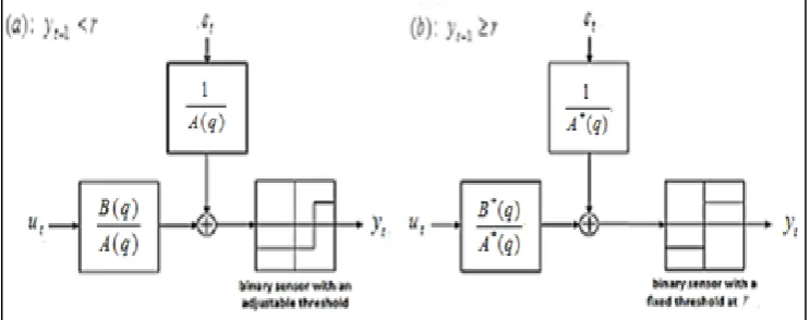
The SETAR model, proved by Kapetanios (14), can be generalized into the threshold ARX model, i.e. SETARX. This can be illustrated in general through the algorithm in Fig.1:

Figure 1. One of the algorithm for the threshold ARX model (15)

Whereas:𝐴(𝑞), 𝐴∗(𝑞) are a polynomial of parameters and back shift operator for the variable 𝑦_𝑡.

𝐵(𝑞), 𝐵∗(𝑞) are a polynomial of parameters and back shift operator for the variable 𝑢𝑡.

𝜀_𝑡 is a prediction error.

Where a simple initial model can be build, as shown in the following equation:(16)

  

 

 



 

 

r y if

r y if y

t t

t

t t

t t

1 1

2

1 1

1

  

  

. . . (5)

Whereas: 𝜃1 the vector of parameters of the model

when 𝑦_𝑡−1< 𝑟.

𝜃₂ the vector of parameters of the model when 𝑦𝑡−1≥ 𝑟.

1 

t



represents the inputs and outputs of the system:









_{ t t t tna t t t tnb}

t1 y y 1 y 2 ... y u u 1 u 2 ... u



The simple model in equation (5) can be generalized into two groups, each group includes

the size of a different sample

n

1

,

n

2so that there will be more than one separation point

)

,

,

,

(

r

₁

r

₂



r

_k , where

k

represents the number of sections separating the two models at a certain point belonging to the points of the depended (exogenous) variable y_tl, and l represents the amount of back shift consequently, the general form of the model will be as follows:

t j t n

j j i

t

i f

y











_











1 ) ( 0

1 . . . (6)

Whereas:

i i

i a b

f

n

n

n





i

a

n Represents the order of the dependent variable

y

, and

i

b

n represents the order of the explanatory

variable

X

, and i1,2,,k.

The model in the equation (6) can be summarized as

follows: ( , , , , )

2 1 f fk

f n n n

k

Comparative Criteria

The criteria below were used to determine the best cut point (threshold) for ARX model by the smallest value of these criteria equivalent to the model. These criteria can also be used to compare between many significant models in the seasonal B-J approach to determine the best significant model.(17, 18, 19)

Akaike's Information Criteria:

Akaike (1973, 1974) used Akaike's information criteria, which is denoted as (AIC), in choosing the suitable order for the models of time series. Its formula is as follows:

𝐴𝐼𝐶(𝑀) = −2 ln 𝐿 + 2𝑀 . . . (7) Whereas M represents the number of the model's parameters, and L is the likelihood function used to estimate the model.

Bayesian Information Criterion:

The general formula for this criterion, which is denoted (BIC), is:

   

 

     

 

  

 

M Ln

M n Ln M

n M Ln M n Ln n M BIC

a Z a

/ 1 ˆ ˆ

) 1 ( ) ( ˆ ) (

2 2 2

  

. . . (8)

Whereas ˆ_Z2 represents the estimation of the

variance time series, and



ˆ

_a2 represents the variance of the residuals time series, and M represents the number of parameters. Akaike suggested that some terms could be neglected to avoid the overestimate order, then the criterion become:

) ( ln ˆ

ln )

(M n 2 M n

BIC  a . . . (9)

Final Prediction Error:

This criterion was used in 1969 by the researcher Akaike and denoted as (FPE). It is calculated according to the variance of prediction error for the next period, its formula is:

FPE = [(1 + M ⁄ n)/(1 − M ⁄ n)] ∗ V . . . (10) Whereas M represents the number of parameters and V represents the loss function and its formula is as follows:

V =1

n ∑ 𝑒𝑡2 . . . (11)

Whereas: 𝑒𝑡 is prediction error and equal: 𝑒𝑡 = 𝑦𝑡−

𝑦̂_𝑡

Mean Square Error:

The mathematical formula of this criterion, which is denoted (MSE), equal to:

n y y MSE   t t

2 ) ˆ

( _{. . . (12)}

Minimize Description Length Criteria:

The mathematical formula of minimizing description length criteria, which is denoted (MDL), equal to:

mod )

( 1

V n

n Log M V

MDL 

  

  

 . . . (13)

Whereas V represents the loss function and M represents the number of parameters inside the model, and

n

represents the size of the sample.

Weighted Comparison Criteria:

In this research, the weighted comparison criteria were proposed using threshold models to determine the general comparison criterion of the data. There is a turning point (cut) where the data will divide into two parts, consequently, a model will be built for each part, and accordingly each part will have a comparison criterion.

If we assume that we have two models: the first has a comparison criterion of, for example, ∆1

with the size 𝑛1, while the second has a comparison

criterion of, for example, ∆₂ with the size 𝑛₂ .

Therefore, it was proposed to use the weighted arithmetic mean in the calculation of the comparison criterion, so we will have the weighted comparison criterion which is denoted (𝑊∆) for the general (total) model of the following equation: 𝑊∆= 𝑊1∗ ∆1+ 𝑊2∗ ∆2 . . . (14)

Whereas 𝑊_𝑖 equals: 𝑊_𝑖 = 𝑛𝑖

𝑛1+𝑛2 ; 𝑖 = 1,2

Equation (14) was used in the comparison criteria AIC, MDL, FPE and MSE.

The Practical Part: Introduction:

Air pollution plays an important role in the air quality management system. The critical periods of the expectations of air pollution are determined by using the relevant weather data in the area with the expectations in the current period. The soils and dust are regarded the main elements in dusty fog in cities, and are among the most complicated pollutants which are difficult to control. This has an important influence on health. In addition, the desert character of the areas surrounding Baghdad caused an increase in the pollution cases of suspended solids, and the increase in storms raised the concentrations of dust in these areas. Further, the low relative humidity and the general average of rain increase the atmospheric lifetime of air pollutants. Consequently, the environmental effects influence human health and cause damage to plants and materials.(20, 21)

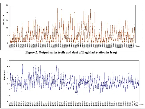
Climate data was taken and analyzed after determining the threshold which separates one period and another by using specific calculations, and the ARX model was built using threshold, for monthly data represented by two climate elements, i.e., soils, dust and wind speed, relating to Baghdad Weather Station for the period from January 1956 until December 2012.

Data Preparation

variable as input series u(t) for the period from January 1956 until December 2012. The data was taken from the Weather Forecast Service of the Ministry of Transportation in Iraq. The data was analyzed by using the MATLAB V.2013a program.

The two Figs.2 and 3 show the nature of the spread of these two series. It is noteworthy that the cross correlation between the two series equals (0.682). This is evidence that there is a correlation between the two variables of this paper.

Figure 2. Output series (soils and dust of Baghdad Station in Iraq)

Figure 3. Input series (wind speed of Baghdad Station in Iraq)

While Fig.4 shows the cross correlation between the two series. There is a system in the

relationship between the two variables as is clear from the change in autocorrelation between them.

The First Method: Determining the Best Cut off Point for Data Modeling by Partial Sizes of Samples

To determine the best ARX model against the best cut point of the study data, the check has been started as of the observation (51); March 1960, [depend on create preliminary ARX model from the initial observations, which are 50 observations, symbolization as n1 and representing from

(December 1956 to February 1960) within determining the model's order, post-taking the combinations (from 1 to 5) of the three different parameters (na, nb, nk)].

Then, searching for the best separation point (threshold point) can be made by dividing the data into two models depending on this point by using some comparison criteria.

This is done through two proposed approaches:

The First Proposed Approach: The Method of Prediction Forward (The Forecasting Approach)

This method depends on the future predictions of the identified models through the following algorithm:

1. Determining the first preliminary separation point, represented by observation 51corresponding to March 1960. Accordingly, the whole sample will be divided into two groups: first group represented by 50 observations, which starts from January 1956 to February 1960, the second group, represented by observations that start with observation 51 until

observation 672, i.e. from March 1969 until December 2012.

2. The best model order of first and second groups are determined by comparing the first 12 observations i.e. the year 1956 forecasted from the first group with the actual observations that from 51 to 62 i.e. from March 1960 to February 1961, and also comparing the first 12 values forecasted from the second group with the actual observations that from 673 to 684 i.e. from September 2003 to December 2012. Then, calculate the comparison of the total model.

3. The cut point is changed by one observation, namely observation 52 i.e. April 1960 and the items mentioned above are calculated again until the last cut point in observation 622 is reached, namely October 2007, where the sample will divide into two groups, the first from observation 1 to 621 observation i.e. from January 1956 to September 2007, the second group represented by observations from 622 to 672 i.e. from October 2007 to December 2011, and compared with the first 12 values for the two samples to calculate the comparison criteria which are AIC, MDL, Loss Function, and MSE criterion.

4. Determining the best cut point and the best model through the smallest measure of comparison to the criteria mentioned in paragraph (3).

The results are as follows: At the AIC criterion:

Table 1. Results of AIC criterion of the first and second groups, and many orders of ARX model, for different sample sizes (The Forecasting Approach)

AIC1 na1 nb1 nk1 n1 AIC2 na2 nb2 nk2 n2 WAIC

1.7655 1 1 2 50 -5.4904 1 4 5 622 -4.9506

-2.3106 2 1 1 52 -5.4909 1 4 5 620 -5.2448

-2.6276 1 3 2 60 -5.7005 1 4 5 612 -5.4261

-4.3528 3 3 3 62 -5.7041 1 4 5 610 -5.5795

-4.4486 1 5 1 71 -5.7408 2 5 4 601 -5.6043

-8.7525 1 4 5 80 -5.9440 2 5 4 592 -6.2783

-6.9916 5 3 1 131 -6.1800 1 5 4 541 -6.3382

-6.5936 5 5 2 496 -5.6604 4 5 5 176 -6.3492

-8.4339 1 3 1 539 -9.1041 5 1 2 133 -8.5666

At the MDL criterion:

Table 2. Results of MDL criterion of the first and second groups, and many orders of ARX model, for different sample sizes (The Forecasting Approach)

MDL1 na1 nb1 nk1 n1 MDL2 na2 nb2 nk2 n2 WMDL

1.8394 1 1 2 50 -5.4556 1 4 5 622 -4.9128

-2.2075 2 1 1 52 -5.4560 1 4 5 620 -5.2046

-2.5037 1 3 2 60 -5.6652 1 4 5 612 -5.3829

-4.1848 3 3 3 62 -5.6687 1 4 5 610 -5.5318

-4.2886 1 5 1 71 -5.6914 2 5 4 601 -5.5431

-8.6210 1 4 5 80 -5.8940 2 5 4 592 -6.2186

-6.8403 5 3 1 131 -6.1338 1 5 4 541 -6.2716

-8.4026 1 3 1 539 -8.9863 5 1 2 133 -8.5181

Table 3. Results of Loss Function of the first and second groups, and many orders of ARX model, for different sample sizes (The Forecasting Approach)

Loss Fun.1 na1 nb1 nk1 n1 Loss Fun.2 na2 nb2 nk2 n2 WLoss .Fun.

1.6481 1 2 1 50 -5.5066 1 4 5 622 -4.9743

-2.4442 2 1 1 52 -5.5072 1 4 5 620 -5.2702

-2.7760 1 3 2 60 -5.7170 1 4 5 612 -5.4544

-4.5605 3 3 3 62 -5.7207 1 4 5 610 -5.6136

-4.6281 1 5 1 71 -5.7642 2 5 4 601 -5.6442

-8.8860 1 4 5 80 -5.9678 2 5 4 592 -6.3152

-7.1158 5 3 1 131 -6.2023 1 5 4 541 -6.3804

-6.6340 5 5 2 496 -5.7634 4 5 5 176 -6.4060

-8.4489 1 3 1 539 -9.1972 5 1 2 133 -8.5970

The results of the weighted comparison criteria in Tables 1, 2, 3 show that the minimum value is (-8.5666, -8.5181, -8.5970) respectively. This corresponds to:

In the first group of observations n1, which

corresponds to the minimum value of those criteria, is when the sample size equals (n1=539), namely the

period from December 1956 to November 2000, at parameters (na=1, nb=3, nk=1) for all comparison criteria used which equal (AIC= -8.4339, MDL= -8.4026, Loss Fun.= -8.4489). The estimation of ARX model equals:

A(q)10.5602q1

Input 1 2 3

0805 . 0 0233 . 0 0556 . 0 )

(q  q  q  q B

And MSE = 11.06

In the second group, which corresponds to the minimum value in the weighted comparison criteria, the sample size is equal (n2=133), namely

the period from December 2000 to December 2011, at parameters (na=5, nb=1, nk=2) for all comparison criteria used which equal (AIC = -9.1041, MDL = -8.9863, Loss Fun.= -9.1972). The estimation of ARX model equals:

5 4

3

2 1

0704 . 0 1574 . 0 2183 . 0

0302 . 0 6019 . 0 1 ) (

 



 

 

 

 

q q

q

q q

q A

Input 2

0485 . 0 )

(q  q

B

And MSE = 7.745

Therefore, the weighted mean square error (WMSE) of the two groups was calculated and equals (10.404).

The Second Proposed Approach: The Method of Prediction from Within the Time Series (The Prediction Approach)

This approach resembles the first approach (the algorithm mentioned in the first approach) with the difference that the comparison is made by predicting from inside the time series of all the first sample whose size is 50 observations, namely January 1956 to February 1960, the second sample is represented by (n-50) which is equal to 634 observations from March 1960 to December 2012. Then, the cut point is changed on the basis that it moves the following observation, namely observation 52 i.e. April 1960, and so on until the last best cut point (threshold) of ARX model is reached.

The results are as follows:

At the AIC criterion:

Table 4. Results of AIC criterion of the first and second groups, and many orders of ARX model, for different sample sizes (The Prediction Approach)

AIC1 na1 nb1 nk1 n1 AIC2 na2 nb2 nk2 n2 WAIC

1.6959 3 1 5 50 2.1970 5 5 5 634 2.1603

1.6852 3 1 4 51 2.1986 5 5 5 633 2.1603

1.6733 3 1 5 52 2.1967 5 5 5 632 2.1569

1.6228 4 4 5 57 2.2041 5 5 5 627 2.1556

1.5965 4 4 5 58 2.2058 5 5 5 626 2.1541

1.5716 4 4 5 59 2.2029 5 5 5 625 2.1484

1.5466 4 4 5 60 2.2011 5 5 5 624 2.1437

1.5223 4 4 5 61 2.2027 5 5 5 623 2.1420

1.6527 4 4 5 75 2.2022 5 5 5 609 2.1420

1.6806 3 1 5 86 2.2068 5 5 5 598 2.1407

1.6702 3 1 5 88 2.2092 5 5 5 596 2.1398

1.6572 3 1 5 89 2.2057 5 5 5 595 2.1344

1.6472 4 4 5 91 2.2081 5 5 5 593 2.1335

1.6339 4 4 5 92 2.2079 5 5 5 592 2.1307

1.6391 4 4 5 93 2.2048 5 5 5 591 2.1279

1.6354 4 4 5 94 2.2050 5 5 5 590 2.1268

1.6229 4 4 5 95 2.2067 5 5 5 589 2.1256

From Table 4 it is obvious that the minimum value of the weighted AIC criterion of data equals (WAIC=2.1253). This corresponds to: In the first group the sample size is equal (n=98), whereas (AIC=1.6171), when the number of parameters is (na=4, nb=4, nk=5). And the estimation of the ARX model is:

4 3 2 1 1734 . 0 2500 . 0 1615 . 0 3959 . 0 1 ) (          q q q q q A Input 8 7 6 5 0724 . 0 0747 . 0 0102 . 0 0258 . 0 ) (         q q q q q B

And MSE = 4.997.

In the second group of observations, which corresponds to the least WAIC, the sample size is equal (N-n1=586) and the criterion value is

(AIC=2.2103), when the number of parameters is (na=5, nb=5, nk=5). And the estimation of the ARX model is: 5 4 3 2 1 0716 . 0 0534 . 0 0845 . 0 0435 . 0 3030 . 0 1 ) (            q q q q q q A Input 9 8 7 6 5 0577 . 0 0299 . 0 0012 . 0 1064 . 0 0316 . 0 ) (           q q q q q q B

And MSE = 8.894.

The WMSE of the two groups equals (8.336).

At the MDL criterion:

Table 5 shows that the minimum value of the weighted MDL criterion equals (WMDL=2.1928). This corresponds to:

Table 5. Results of MDL criterion of the first and second groups, and many orders of ARX model, for different sample sizes (The Prediction Approach)

MDL1 na1 nb1 nk1 n1 MDL2 na2 nb2 nk2 n2 WMDL

1.8071 1 1 5 50 2.2549 1 4 5 634 2.2222

1.7859 1 1 5 51 2.2566 1 4 5 633 2.2215

1.7640 1 1 5 52 2.2558 1 4 5 632 2.2184

1.7142 1 1 5 58 2.2648 1 4 5 626 2.2182

1.6926 1 1 5 59 2.2626 1 4 5 625 2.2134

1.6712 1 1 5 60 2.2601 1 4 5 624 2.2084

1.6510 1 1 5 61 2.2618 1 4 5 623 2.2073

1.7579 1 1 5 84 2.2699 1 4 5 600 2.2070

1.7563 1 1 5 86 2.2689 1 4 5 598 2.2045

1.7478 1 1 5 87 2.2707 1 4 5 597 2.2042

1.7373 1 1 5 88 2.2724 1 4 5 596 2.2035

1.7254 1 1 5 89 2.2694 1 4 5 595 2.1986

1.7145 1 1 5 92 2.2724 1 4 5 592 2.1974

1.7263 1 1 5 93 2.2672 1 4 5 591 2.1936

1.7227 1 1 5 95 2.2687 1 4 5 589 2.1928

In the first group, the sample size is equal (n=95), and (MDL=1.7227), when the number of parameters is (na=1, nb=1, nk=5). And the estimation of the ARX model is:

1 3884 . 0 1 )

(q   q A

Input B(q)0.0460q5

And MSE = 5.049

As for the results of the second group, it will be at the sample size (N-n1=589) which corresponds

to (MDL=2.2687) when the number of parameters

(na=1,nb=4, nk=5).And the estimation of the ARX model is: 1 3797 . 0 1 )

(q   q A Input 8 7 6 5 0628 . 0 05 387 . 9 1170 . 0 0195 . 0 ) (          q q E q q q B

And MSE = 9.182

The WMSE of the two groups was calculated and equals (8.608).

Table 6. Results of Loss Function criterion of the first and second groups, and many orders of ARX model, for different sample sizes (The Prediction Approach)

Loss Fun.1 na1 nb1 nk1 n1 Loss Fun.2 na2 nb2 nk2 n2 WLoss. Fun.

1.3588 5 5 5 50 2.1654 5 5 5 634 2.1065

1.3550 5 5 4 51 2.1670 5 5 5 633 2.1064

1.3629 5 5 4 52 2.1650 5 5 5 632 2.1040

1.3518 5 5 4 53 2.1666 5 5 5 631 2.1035

1.3353 5 5 4 54 2.1681 5 5 5 630 2.1024

1.3250 5 5 4 56 2.1712 5 5 5 628 2.1019

1.3116 5 5 4 57 2.1722 5 5 5 627 2.1005

1.2906 5 5 4 58 2.1738 5 5 5 626 2.0989

1.2711 5 5 4 59 2.1709 5 5 5 625 2.0933

1.2509 5 5 4 60 2.1691 5 5 5 624 2.0885

1.2313 5 5 4 61 2.1706 5 5 5 623 2.0868

1.4129 5 5 5 75 2.1694 5 5 5 609 2.0864

1.4794 5 5 5 88 2.1756 5 5 5 596 2.0860

1.4673 5 5 5 89 2.1721 5 5 5 595 2.0804

1.4547 5 5 5 91 2.1744 5 5 5 593 2.0786

1.4435 5 5 5 92 2.1741 5 5 5 592 2.0759

1.4492 5 5 5 93 2.1709 5 5 5 591 2.0728

1.4465 5 5 5 94 2.1711 5 5 5 590 2.0716

1.4354 5 5 5 95 2.1727 5 5 5 589 2.0703

1.4378 5 5 4 97 2.1745 5 5 5 587 2.0700

1.4306 5 5 4 98 2.1762 5 5 5 586 2.0694

2.2203 5 5 5 489 1.6884 5 5 5 195 2.0687

Table 6 shows that the minimum value of the weighted loss function (WLoss Fun.) is equal (2.0687) which corresponds to the following:

In the first group of data has a sample size of (n=489) and (Loss. Fun.= 2.2203), when the number of parameters is (na=5, nb=5, nk= 5). And the estimation of ARX model is equal to:

3 4 5

2 1 0557 . 0 0930 . 0 0237 . 0 0951 . 0 3376 . 0 1 ) (            q q q q q q A Input 9 8 7 6 5 0392 . 0 0637 . 0 0269 . 0 0842 . 0 0368 . 0 ) (           q q q q q q B

And MSE = 9.364

As for the second group of data, it will be at the sample size (N-n1 = 195) and (Loss. Fun.=

1.6884), when the number of parameters (na=5, nb= 5, nk=5). And the estimation of ARX model is equal to: 5 4 3 2 1 1220 . 0 0347 . 0 2047 . 0 1579 . 0 3117 . 0 1 ) (            q q q q q q A Input 9 8 7 6 5 1050 . 0 0858 . 0 0647 . 0 1169 . 0 0252 . 0 ) (           q q q q q q B

And MSE = 5.995

And the value of WMSE for the results of two groups is equal to (8.404)

The second method: Determine the Size of the Sample Using the Seasonal B-J Models

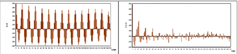
From Fig.2 for the soils and dust series of the Baghdad Station in Iraq, and Fig.5 for the autocorrelation (AC) and the partial autocorrelation (PAC) respectively by using SPSS V.20 program, it is clear that there is no stationary due to the sharp curves in the series data.

In the Dickey-Feller test, it shows stationary in the time series, although the series is found to be non-stationary when looking at the AC and PAC. Indicating the ratio of outliers values in the series so that they do not affect the total size of the sample in terms of stationary. Where the p-value is less than 0.05 for all test models shown in the Table 7, this confirms that the series is stationary.

Table 7. Dickey-Feller test for soils and dust series of Baghdad Station

P-Value Test

Input Output

0.0003 8.735E-006

Constant

0.0008 8.1296E-005

Constant and trend

The most important tests used in seasonal pattern detection are Kruskal-Wallis and Jonckheere-Terpstra tests. The hypothesis of the test is as follows:

H0: There is no seasonal in the data

H1: There is seasonal in the data

The results are as follows:

Table 8. Kruskal-Wallis and Jonckheere-Terpstra test of soils and dust data at Baghdad Station

The results of the Table 8 show that the null hypothesis is rejected at a significant level of 0.05, i.e., the seasonal data containment that occurs every 12 months.

Thus, a number of seasonal B-J models (i.e. seasonal autoregressive integrated moving average SARIMA model) have been applied to the data using MATLAB V.2013a program, through two approaches:

The First Approach: (The Forecasting

Approach)

In this approach, a 7560 seasonal models are tested. The program has been implemented continuously (i.e. is the implementation period of the program and not the period of the building). The best order were selected according to the minimum value of the comparison criteria using the forecasting principle of 12 observations forward, i.e. adopt a sample size of 672 out of 684 observations. This technique can be called a

(Sample Test). The results are shown in Table 9.

Table 9. The significant models of seasonal B-J with the corresponding comparison criteria by testing a sample of 672 observations by (Forecasting Approach) (Sample Test)

n1 P q P Q s D D AIC1 BIC1 FPE1 MDL1

In the Table 9, it is found that the minimum values for the comparison criteria in the SARIMA(0,0,2)(3,0,0)12 model in which

the values of: AIC= 3648.3771, BIC= 3656.6205, FPE= 21.0409, MDL= 19.6781 .

Thus, this seasonal model was selected for (Sample Testing), where the value of MSE= 12.1850

The estimation of the parameters of this seasonal model is shown in the Table 10:

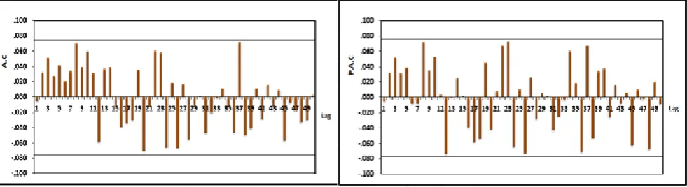
When testing the accuracy of the model, the following Fig.6 illustrates the randomized model and AC and PAC coefficients of the residuals are located within the confidence interval and equal to{±0.075}.

Table 10. Estimating the parameters of the SARIMA(0,0,2)(3,0,0)12 model in

(Forecasting Approach/Sample Test)

Sig. t-statistic S.E

Estimate Parameters

0.000 -7.587

0.039 -0.292

MA(1)

0.000 -4.556

0.039 -0.176

MA(2)

0.000 8.726

0.038 0.328

SAR(1)

0.000 7.055

0.039 0.273

SAR(2)

0.000 6.928

0.038 0.265

SAR(3)

The value of the statistic Q Ljung-Box =

45.444 and compared with the value of 2 _tabular

and degree of freedom (45) and significant level (0.05) is equal to (61.3850), it is clear that the model is appropriate to represent the data.

Figure 6. AC and PAC coefficients for the residuals of the SARIMA(0,0,2)(3,0,0)12 model

The combinations (0 to 5) were taken for each of the four parameters model (p, q, P, Q), and the results are shown in Table 11 and this technique can be called a (Sample Estimation).

The Second Approach: (The Prediction

Approach)

In this method, 7560 seasonal models were tested through test 684 observations as a sample, these observations are predicted within the series and all the criteria are shown to be consistent with a seasonal model (s = 12).

Table 11. The significant models of seasonal B-J with the corresponding comparison criteria by testing a sample of 684 observations in (Prediction Approach) (Sample Estimation)

n P Q P Q S d D AIC BIC FPE MDL

The Table 11 shows that the minimum values of the comparison criteria in the SARIMA(0,0,4)(5,0,0)12 model, where:

AIC= 3603.7173, BIC= 3644.4689, FPE= 22.4349, MDL= 12.0228

Thus, this seasonal model was selected for (Sample Estimation), where the value of MSE=11.0718 The estimation of the parameters of this seasonal model is given in the Table 12:

Table 12. Estimating the parameters of the SARIMA(0,0,4)(5,0,0)12 model for (Prediction

Approach) (Sample Estimation)

Sig. t-statistic S. E

Estimate Parameters

0.000 -7.596

0.038 -0.291

MA(1)

0.000 -5.321

0.039 -0.209

MA(2)

0.000 -4.666

0.039 -0.183

MA(3)

0.000 -4.505

0.038 -0.172

MA(4)

0.000 6.459

0.038 0.248

SAR(1)

0.000 5.171

0.040 0.204

SAR(2)

0.000 4.494

0.040 0.180

SAR(3)

0.009 2.564

0.040 0.103

SAR(4)

.0000 3.593

.0400 .1420

SAR(5)

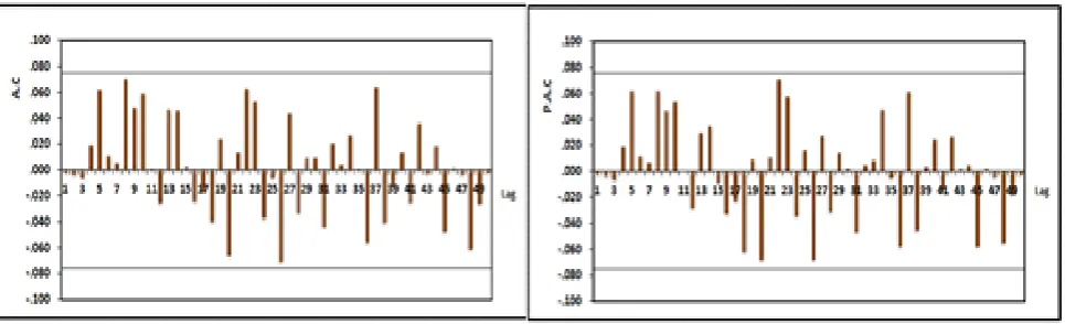
When testing the accuracy of the model, the Fig.7 illustrates the randomized model and AC, PAC coefficients of the residuals are within the confidence interval and its: {±0.075}

Figure 7. AC and PAC coefficients for the residuals of the SARIMA(0,0,4)(5,0,0)12 model

By comparing the value Q Ljung-Box = 21.107

with 2 _{tabular at a d.f = 41 and a significant level}

of 0.05 it’s equal to (56.9350), it is clear that the model is appropriate to represent the data.

Conclusions:

1- All the comparison criteria used in the forecasting method agree on the size of a sample at a certain threshold and agreed on the same number of parameters used to estimate the model at each threshold. Thus, this method can be considered more stable in determining the threshold point and the order of the ARX model. 2- There is a slight variation in the results of the

comparison criteria (AIC and MDL) used in the predictive method within the series in terms of sample size at a certain threshold, as opposed to the results of the loss function in which a large difference in sample size appears at a given threshold. The number of parameters shows the specific values of the orders differed according to the criteria used.

3- The last threshold changes the function when the first approach (Forecasting) is at the threshold

size of the sample 539, then the ARX model is stabilized and unchanged until the last observation.

4- The results show that the best cut-off model is determined by the second approach (Prediction) at the AIC criterion where WMSE = 8.336 followed by the use of the loss function in which WMSE = 8.404, while MLD criterion is the last and WMSE = 8.608.

5- Through the results of the weighted mean square error, it is clear that the second approach is the best in determining the best threshold point for modeling and equal to 8.336 while its value is equal to 10.404 when using the first approach. 6- When using the first approach of sample

determination using seasonal B-J models, the SARIMA(0,0,2)(3,0,0)12 model is the best fit for

time series data depending on a sample of 672 out of 684 observations (according to the principle of forecasting the 12-observation forward).

the best fit for time series data depending on the total sample size.

8- When comparing the results of the two approaches of the seasonal B-J models, it is clear that the second approach in which MSE=11.0718 is better than using the first approach in which MSE= 12.1850.

9- When comparing all the results of the research, it is clear that the first method (i.e., determining the best cut off point for data modeling by partial sizes of samples) is preferable to the second method, which includes sample size determination using seasonal B-J models.

10- The results of the research also indicate that the second approach (Prediction) is the best in determining the best threshold point during which the data can be divided into two models through that point. This indicates that the approach of prediction from within the series of threshold ARX model is the best performed compared to the SARIMA models.

Recommendations

1- From the results, more than one threshold has been maintained for a long time. Therefore, we recommend studying the case of more than a threshold within one group of time series data. 2- By drawing the time series, some values were

observed beyond the limits of control. The Dickey-Fuller test found that the series in its general form was stationary. This indicates that the ratio of the number of outliers to the size of the sample has a direct effect on the decision that the series is stationary or not. Therefore, we recommend studying the effect of the number of outliers' values on the size of the sample and its effect on the stationary decision of the time series.

3- Using nonlinear models for the threshold ARX model.

4- Using a multiple inputs with single output system (MISO) with the threshold problem.

5- Using a multiple inputs with multiple outputs system (MIMO) with the threshold problem. 6- Using the threshold ARX model on the basis of

each section (sample) on both sides of the threshold point is represented by a seasonal model and with determined orders.

7- For a large number of sources of air pollution from the environment, domestic and industrial...., so a particular network must be done to monitor the type of pollution in a particular area.

References:

1. Chatfield C. The analysis of time series an introduction. 6th ed. Chapman & Hall/CRC. By Taylor& Francis Group.2003.

2. Franses PH, Dijk DV. Nonlinear time series models in empirical finance. Cambridge University Press. 2000. 3. Granger CWJ, Terasvirta T. Modelling nonlinear economic relationships. Oxford University Press. 1993.

4. Chen R, Tsay RS. Nonlinear additive ARX models,

Journal of the American Statistical Association. 1993 September; 88(423):955-967.

5. Lucheroni C. TARX models for spikes and antispikes in electricity markets. Conference Paper in SSRN Electronic Journal. Source: IEEE Xplore. 2010 July: 1-7. DOI:10.1109/EEM.2010.5558724.

6. Frimpong JM, Oteng-Abayie EF. When is inflation harmful? Estimating the threshold effect for Ghana.

American Journal of Economics and Business Administration. 2010; 2 (3): 232-239.

7. Filipovic V, Stojanovic V, Nedic N, Prsic D. TARX model of pneumatic cylinder and identification. Conference Paper: Conference: SAUM, At Nis, Serbia, V.: XI International Conference on Systems, Automatic Control and Measurements. 2012 November; 260-263.

8. Tsay RS. Analysis of financial time series. John Wiley & Sons, 2nd edition, New-Jersey.2001.

9. Tong, H. Nonlinear time series: A dynamical system approach. Oxford University Press Inc. New York.1990

10. Li Z. Autoregression models for trust management in wireless Ad Hoc networks. Thesis, School of Electrical Engineering & Computer Science, University of Ottawapp, Canada. 2011:1-84.

11. Ohlsson H , Ljung L, Boyd S. Segmentation of ARX-models using sum-of-norms regularization. Automatica. 2010; 46(6):1107-1111.June.

12. Knotters M, Bierkens MFP. Physical basis of time series models for water table depths. Water Resources. Research 2000 Janury; 36(1):181-188. 13. Al-Talib M S. Employing ridge regression technique

in prediction of the black box models with application. Iraqi Journal of Statistical Science.2012; 22: 121-135.

14. Kapetanios, G. Threshold models for trended time series. Empirical Economics. 2003; 28(4):687-707. Springer. DOI 10.1007/s00181-003-0154-8

15. Cs´aji BC, Weyer E. Recursive estimation of ARX systems using binary sensors with adjustable thresholds. Preprints of the 16th IFAC Symposium on System Identification, Brussels, Belgium. 2012July;45(16):1185-1190.

18. Akaike H . A bayesian extension of the minimum AIC procedure of autoregressive model fitting. Biometrika.1979 August; 66(2):237-242.

19. Makridakis S, Wheelwrighrt SC,Hyndman R. Forecasting methods and application. John Wiley & Sons, Inc. New-York.1998

20. Al-Tahi W KJ. Environmental pollution and green economy. Ministry of finance. Economic circle,

Economic policy department.1-25. http://www.mof.gov.iq/Lists/ResearchesAndStudies/t louth.pdf

21. Kim SE, Kumar A. Accounting seasonal nonstationarity in time series models for short-term ozone level forecast. Stochastic Environmental Research and Risk Assessment. 2005 October; 19(4): 241–248.

ةقيرط

ةروـَّطم

مادختساب

ؤبنتلا

يف

ءانب

لضفا

جذومنا

ةبتع

ــل

ARX

عم

قيبطت

يلمع

ملاحا

دمحا

ةعمج

1

سارف

دمحا

دمحم

انهملا

2

1

مسق ملع عامتجلاا ، ةيلك بادلآا ،دادغب ،دادغب ةعماج ، قارعلا

.

2

مسق ءاصحلاا ، داصتقلااو ةرادلاا ةيلك ،

دادغب ةعماج ،دادغب ،

قارعلا

.

لا

ةصلاخ

:

فلتخمل ؤبنتلا ةيلمع يف ةعساولا اهتيناكماب زيمتت يتلاو ةينمزلا لسلاسلا ليلحت يف ةمهملا قرطلا نم ةيطخلا ريغ جذامنلا ربتعت اصخ ةسارد للاخ نم ،ةيداصتقلااو ةيسدنهلاو ةيئايزيفلا اهنم رهاوظلا ؤبنتلا ىلا لصوتلل اهيف ةيئاوشعلا تابارطضلاا صئ

.قيقد لكشب تا

مت ثحبلا اذه يفو ب

جذومنا ءان يجراخ اريغتم عم يتاذ رادحنا

ةبتعلا مادختساب Threshold

مت نيحرتقم نيبولسا للاخ نم ،ىلوا ةقيرطك

امه )ةبتع( عطق ةطقن لضفا ديدحت ضرغل امهفيظوت ]

( ماملاا ىلا ؤبنتلا Forecasting

( ةينمزلا ةلسلسلا لخاد نم ؤبنتلاو ) Prediction

)

ةبتعلا ةطقن رشؤم للاخ نم [

. جذامن مادختسا ىلا ةفاضلااب B-J

يف نيحرتقملا نيبولسلاا أدبم ىلع ًادامتعا ةيناث ةقيرطك ةيدايتعلاا ةيمسوملا

.يمسوم جذومنا لضفا ديدحت ةنراقملاو

عم جذامنلا ةلصحتسملا اهيلع

نم نيبولسلاا ةروكذملا

هلاعا ،نيتقيرطلل نم

للاخ ةعومجم نم

ريياعملا يهو AIC ، MDL ، Loss Function ،

BIC ، FPE ، MSE ةفاضلااب ىلا ريياعم ةنراقملا نوزوملا Weighted Comparison

Criteria ،ةحرتقملا

ديدحتل لضفا جذومنا ليثمتل تانايب ثحبلا ةلثمتملاو ةعرسب

حايرلا ريغتمك لخدم ةبرتلااو رابغلاو ريغتمك جرخم

ةصاخلاو ةطحمب

دادغب ةرتفلل نم رهش نوناك يناثلا 1956 ةياغلو رهش نوناك لولاا 2012 .

ةيحاتفملا تاملكلا

: ARX ،ؤبنتلا ،يلبقتسملا ؤبنتلا ، يتاذلا رادحنلاا

،لماكتملا كرحتملا طسوتملا ةبتعلا