A New Multivariate Weibull Distribution

(1)

Saman Hanif Shahbaz

Department of Statistics, Faculty of Science King Abdulaziz University, Jeddah, Saudi Arabia [email protected]

Mashail Al–Sobhi

Department of Mathematics

Umm Al–Qura University, Makkah, Saudi Arabia [email protected]

Muhammad Qaiser Shahbaz

Bander Al–Zahrani

Abstract

We h a v e proposed a new multivariate Weibull distribution as a compound distribution of univariate Weibull distributions. We have studied some properties of the proposed distribution. The multivariate distribution of records for proposed distribution has also been studied. Estimation of the parameters has been done alongside application to the real data set.

Keywords: Moments of residual life, Goodness-of-fit, Order Statistics, Maximum Likelihood Estimation.

Introduction

Weibull distribution, introduced by Weibull (1951), has been a popular model for modelling the lifetime data. The density and distribution function of Weibull distribution can be presented in various ways, see for example Johnson et al. (1995). A relatively simple form of the density function is





1





; , exp ; , , 0.

f x  x x x   (1)

The distribution function corresponding to (1) is



; ,



1 exp





; , , 0.

F x    x x   (2)

(2)

Beta-Weibull distribution. Cordeiro et al. (2010) have proposed the Kumaraswamy-Beta-Weibull distribution as an alternative to Weibull distribution with much wider applicability.

Chandler (1952) introduced record statistics as a model for ordered random variables. The records are defined in a sequence of independent and identically distributed random variables as under.

Suppose a sequence of independently and identically distributed random variables

1, 2, , n

X X  X is available with same distribution function F x . Suppose further that

 



1 2



max , , ,

n n

Y  X X  X for n1, then X_j is an Upper Record Value of the sequence



X_n,n1



if Yj Yj1. From this definition it is clear that X is an upper record value.1

We also associate the indices to each record value with which they occur. These indices are called the record time



U n

 

,n0



where

 

min



|



1 ,



j U n 1, 1



U n  j j U n X X _ n .

We can readily see that U

 

1 1. The upper record values are denoted by X n

 

. The density function of nth upper record statistics is given by Chandler (1952) as

 

   

 

1

; .

n X n

f x R x f x x

n



 _ _     

 (3)

The joint density function of mth and nth upper records is given by Chandler (1952) as

   





  

      

 

1

1 2 1 2 1

,

1

2 1 1 2

1 ,

; 4

m X m X n

n m

f x x r x f x R x

m n m

R x R x x x



 

 _ _

  

_  _      

where R x

 

 ln 1



F x

 



and

 

/

 



 



1

r x R x  f x F x .

Record statistics has been studied by several authors for various probability distributions. Ahsanullah (1992) has provided general results for distribution of records for continuous probability distributions. A comprehensive review of record statistics can be found in Ahsanullah (1995) and Nevzorov (2001). Often we have a sample from some bivariate distribution and the sample is arranged with respect to one of the variable. The automatically shuffled other variable is called concomitant of ordered variable. The concomitant of records appear when the bivariate sample is arranged with respect to records. The density function of nth concomitant of record is given by Ahsanullah (1995) as

 



|



X n 

 

Y n

f_ _ y  f y x f x dx

  



 (5)

where f_{X n}_{ }

 

x is defined in (3). The joint distribution of two concomitants of record values is given by Ahsanullah (1995) as

   







 



   





1

1 2 1 1 2 2 , 1 2 2 1

, , | | X m X n , Y m Y n _x

f_ _ y y   f y x f y x f x x dx dx

(3)

where f_{X m X n}_{   }_,



x x₁, ₂



is given in (4). Distribution of concomitants of records for various distributions has been studied by many authors. Shahbaz et al. (2011) have studied concomitants of record statistics for a new bivariate Weibull distribution.

The distribution of concomitants has been extended to bivariate case by Shahbaz et al. (2012). The density function of nth bivariate record statistics is given as

   ,

 

,



, |



X n 

 

Y n Z n

f_ _ y z  f y z x f x dx

  



 , (7)

where f y z x



, |



is the conditional distribution of Y and Z given X = x. Shahbaz et al. (2014) and Shahbaz et al. (2012) have studied bivariate concomitants of records for trivariate Weibull and trivariate Inverse Weibull distribution.

Recently Arnold et al. (2009) have introduced ordering of vectors by using the distribution of concomitants. The distribution of multivariate concomitants is given by Arnold et al. (2009) as

 n

 



|



X n 

 

f_ _  f x f x dx

y  y 



 y (8)

where f



y|x



is the conditional distribution of vector y given X and f_{X n}_{ }

 

x is defined

in (3).

In this paper we have proposed a new multivariate Weibull distribution and have studied its properties. The new multivariate distribution is proposed in section 2 with some graphical study. In section 3 some common properties of the proposed distribution has been studied. Multivariate concomitants of the distribution has been studied in section 4. Application of proposed distribution is given in section 5.

The New Multivariate Weibull Distribution

Shahbaz et al. (2012) has proposed a trivariate Weibull distribution by using compounding of distributions. The density function of proposed trivariate Weibull distribution is





  



 









 





 

3

1 2

3

1 1

1 1 1 1 2 1 2 3 1 2 1 1 2

1 1 2 1 2

1 2 1 1 2 1 2 3

, , ,

exp , ,

0 ; , 0 ; , , , , , 0, 9

f x z z x x z x z z

x x z x z z

  



 

    

 

    

  



 

 _   _

  

where₁

 

x is some function of X and₂



x z, ₁



is some function of X and Z1. Shahbaz et

al. (2012) have used

 

1

1 x x



  and





1 2

2 x z, 1 x z1

 

  to propose following specific

density function





3 1 1 2 2 1 3 1 1



1 2 3



1 2 1 2 3 1 2 1 1 2

, , exp 1 ,

(4)

Suppose X has a Weibull distribution with density function





1

 

; exp ; , 0

f x  x x x   . (11)

We write X has W

 

1, . Now suppose that Y x has₁| W



₁

 

x ,₁



, Y₂|



x y, ₁



has







2 , 1 , 2



W  x y  , Y₃|



x y y, ₁, ₂



has W



₃



x y y, ₁, ₂



,₃



and so on, such that



1 2 1



| , , , ,

p p

Y x y y  y _ has W



p



x y y, 1, 2,yp1



,p



with densities





 



 



































1 1 2 2 3 3 1

1 1 1 1 1 1

1

2 1 2 2 1 2 2 1 2

1

3 1 2 3 3 1 2 3 3 1 2 3

| exp

| , , exp ,

| , , , , exp , ,

f y x x y x y

f y x y x y y x y y

f y x y y x y y y x y y y

                        and









3 1









1 1 1 1 3 1 1

| , , , , , exp , , , p ,

p p p p p p p p

f y x y y    x y  y  y   x y  y  y

where _i 0 and _i

 

x,. 0 ;i1, 2,,p. For simplicity we use



i| , i1



i i



, i 1



exp



i



, i1



i



; 1, 2, , , f y x y_   x y _  x y_ y i  p

where ₁



x,y₀



₁

  

x ,₂ x,y₁



₂



x y, ₁

 

,₃ x,y₂



₃



x y y, ₁, ₂



and so on. Now the density function of



p 1



variate distribution is

 

,

 

₁



| , 1



,

p

i i i

f x y  f x 



_ f y x y_

where y y1 y2  yp. Using above densities, the density function of



p 1



variate Weibull distribution is

 

1

 













1 1

1

, exp p _{i i} , _i exp _i , _i _i ,

i

f x y x x 



_  x y_  x y_ y (12)

where x y, _i 0. The distribution (12) can be studied for various choices of _i



x,y_i_₁



. In this paper we have studied the distribution (12) for following choices of _i



x,y_i_₁



 





1





1 2

1 x x , 2 x y, 1 x y1 , 3 x y y, 1, 2 x y y1 2

  

  

      and





1 1

1 1 1 1

, , , p

p x y yp x y yp

  

 

  

  . Using these in (12), the density function of



p 1



variate Weibull distribution is

 





















1 1

3 3

1 2 1 2 1 2 1 2

3 3

1 2 1 2

1 1

1 1 1

1 1

2 1 2 1 2 3 1 2 3 1 2 3

1

3 1 2 3 1 2 3

, exp exp

exp exp

exp p

p

f x x x x y x y

x y y x y y x y y y x y y y

x y y y x y y y y

                                                  y    or

 





 



 







 

1 1 1 1

1 1

,

exp 1 , 13

i

j

p _p p _p _i

i i i i i p j i j

f x x y

(5)

with x0 and y0. The joint marginal distribution of y is readily obtained as

 





 



 







1 1 1 1

1 1

0 0

1 1

,

exp 1 ,

i

j

p p p p i

i i i i i p j i j

f f x dx x y

x y dx

        _ _ _{ } _            __  __





 

y y

which after simplification becomes

 





 









1 1 1 1 1 1 1

; 0 , 0.

1

i

j

p p _p _i i i i i i p i p j i j p y f y                 



 

y y (14)

The marginal distribution of ith component of y is

 







 







1 1 1

0 0 0 0

1 1

1 1 1

1 0 0 0 0

1 1

1

i

j

i i p p

p p p i i i i i

i i p p

i p

j i j

f y f dy dy dy dy

p y

dy dy dy dy

y                           

   



   

 

y      

which after simplification become

 





1

2 ; , 0.

1

i

i i

i i i

i

y

f y y

y     _    (15)

The joint marginal distribution of any pair



y y_i, _k



is given as

 







 







1 1 1 1 1

0 0 0 0 0 0

1 1

1 0 0 0 0 0 0

1 1

1 1 1 1 1

1

,

i

j

i i i k k p

p p _p _i i i i i p i p j i j i i k k p

f y f dy dy dy dy dy dy

p y

y

dy dy dy dy dy dy

                      _ _            

     



     

 

y            









2 1 1 3

2

, ; , , , 0.

1

i k

i i k

i k i k

i k i k i k

i i k

y y

f y y y y

y y y

 

  

    _{ }

 

  (16)

We now obtain the entries of mean vector and covariance matrix of yas under.

The qth moment of Yiis

 





1 2 0 0 1

1 ; .

i

q q q i i i i i i i i

i i i i i

y

E Y y f y dy y dy

y

q q q

q                   _ _{ }  _     



Using q = 1, the ith entry of mean vector of Yiis

 

1 1 1

1 ; 1.

i i

i i i

E Y 

  

   

 _ _{ }  _ 

(6)

Further, using q = 2, we have

 

2 2 2 2

1 ; 2.

i i

i i i

E Y 

  

   

 _ _{ }  _ 

    (18)

The variance can be easily obtained from (17) and (18). Further













2 1 1 3

0 0 0 0

2

, ,

1

i k

i i k

i k i k

i k i k i k i k i k i k i i k

y y

E Y Y y y f y y dy dy y y dy dy

y y y

                

 





1 1 1 1

1 1 1 ; 1 , 1.

i k i k

i k i k

E Y Y  

   

     

  _ _{ }  _{ }   _  

      (19)

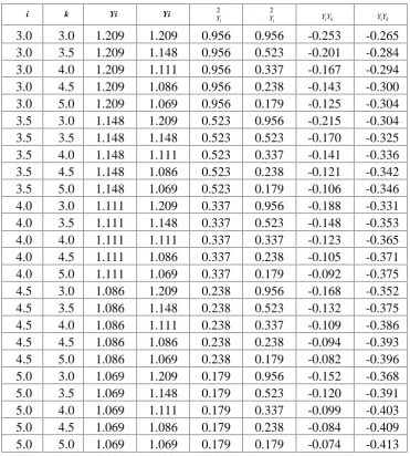
The covariance can be obtained from (17) and (19). Following table contains means, variances, covariances and correlations between Yi and Yk for selected values of i and

k

 . From the table we can see that that the means, variances, covariances and correlations decrease with increase in i and k.

Further, the joint conditional distribution of y given X = x is obtained from (11) and (13) and is given as





 







 







 

1 1 1 1 1 1 , |

exp 1 . 20

i

j

p p p p i

i i i i i p j i j f x

f x x y

f x x y                    _  _  



 

y y

The conditional moments of order q for distribution (20) are given as





1

| qp 1 .

q q

E Y x x 



  

  _ _

  (21)

and



2



1

| 1 ; ; 2,3, , .

q

i i

p q q

E Y x  q i p

  

   

 _ _{ }  _  

 

   (22)

The conditional means and conditional variances can be computed from (21) and (22). Further, the joint conditional moments for distribution (20) are













1 1 1 2

2 1 2 2

1 3

1 3 1 3 2

1 1 1 1

| 1

1 1 1 1

| 1

1 1 1 1

| 1 1 1 ; 1 , 3.

i k

i k i k

E Y Y x x

E Y Y x i k

                         _  _{ } _            _ __ _ _ _               _ _{ }  _{ }   _        

The conditional mean vector and covariance matrix can be computed for specific values of i, k, and x.

(7)

Table 1: Means, Variances and Covariance

αi αk μYi μYi 2

i

Y

σ 2

i

Y

σ σY Y_{i k} ρY Yi k

3.0 3.0 1.209 1.209 0.956 0.956 -0.253 -0.265

3.0 3.5 1.209 1.148 0.956 0.523 -0.201 -0.284

3.0 4.0 1.209 1.111 0.956 0.337 -0.167 -0.294

3.0 4.5 1.209 1.086 0.956 0.238 -0.143 -0.300

3.0 5.0 1.209 1.069 0.956 0.179 -0.125 -0.304

3.5 3.0 1.148 1.209 0.523 0.956 -0.215 -0.304

3.5 3.5 1.148 1.148 0.523 0.523 -0.170 -0.325

3.5 4.0 1.148 1.111 0.523 0.337 -0.141 -0.336

3.5 4.5 1.148 1.086 0.523 0.238 -0.121 -0.342

3.5 5.0 1.148 1.069 0.523 0.179 -0.106 -0.346

4.0 3.0 1.111 1.209 0.337 0.956 -0.188 -0.331

4.0 3.5 1.111 1.148 0.337 0.523 -0.148 -0.353

4.0 4.0 1.111 1.111 0.337 0.337 -0.123 -0.365

4.0 4.5 1.111 1.086 0.337 0.238 -0.105 -0.371

4.0 5.0 1.111 1.069 0.337 0.179 -0.092 -0.375

4.5 3.0 1.086 1.209 0.238 0.956 -0.168 -0.352

4.5 3.5 1.086 1.148 0.238 0.523 -0.132 -0.375

4.5 4.0 1.086 1.111 0.238 0.337 -0.109 -0.386

4.5 4.5 1.086 1.086 0.238 0.238 -0.094 -0.393

4.5 5.0 1.086 1.069 0.238 0.179 -0.082 -0.396

5.0 3.0 1.069 1.209 0.179 0.956 -0.152 -0.368

5.0 3.5 1.069 1.148 0.179 0.523 -0.120 -0.391

5.0 4.0 1.069 1.111 0.179 0.337 -0.099 -0.403

5.0 4.5 1.069 1.086 0.179 0.238 -0.084 -0.409

5.0 5.0 1.069 1.069 0.179 0.179 -0.074 -0.413

Distribution of Multivariate Concomitants

The concomitants of record values have been studied by several authors. Shahbaz et al. (2012) have studied the bivariate concomitants of record values for a trivariate Weibull distribution. Arnold et al. (2009) have provided the distribution of multivariate concomitants of record values which is given in (8) as

 n

 



|



X n 

 

,

f_ _  f x f x dx 

y  y 



y

where

 

   

 

1

; .

n X n

f x R x f x x

n



 _ _     



(8)

the conditional distribution of y given x is given in (20). Now for distribution (11) we have

 

1 exp

 

; 0

F x   x x , so

 

ln 1

 

,

R x    _ F x  _ x and

 

n 1exp

 

. X n

f x x x

n

 

 

 

 (23)

Now using (20) and (23) in (8), the distribution of multivariate concomitant of order statistics for new multivariate Weibull distribution is obtained as under

 





 



 







1 1 1

1 1 0 1 1 exp 1 i j

p p n p p i

i i

n i i

i p

j i j

f x y

n

x y dx

      _ _ _ _{ } _                _  _  





 

y y or

 



1





1  1  1



0   1exp



1 1 1



j i

p p p i p n p i

i i j

n i i i j

f y x x y dx

n



  

 _ _{ } _  _ _

     

y  y _





 







 



 







 













1 1 1 1 1 1 ; 0 1 i j

p p p i i i i i

i

n n p

i p j i j y n p f y n y                     _



 

y y . (24)

The marginal distribution of ith concomitant is readily written from (24) as

 





1 ; 0 1 i i i i i i i

Y n n p i

n y

f y y

y             .

The joint marginal distribution of two concomitants is obtained from (24) as

   













2 1 1

, 2

1

, ; , 0

1

i k

i i k

i k i k

Y n Y n n

i i k

n n y y

f y y y y

y y y

                

  . (25)

The qth moment of ith concomitant is readily obtained from (24) as

 

1

1 ;

q

i i n

i i

q q q

E Y n

n    n

   

  _ _{ }  _  

 _ _{ } _ (26)

The mean and variance can be easily obtained from (26). Further, the product moment between ith and kth concomitant is

   





 

1 1 1 1 1

1 1

i n k n

i k i k

E Y Y n

n    

     

 _  _{ }  _{ }   _

(9)

The covariance con be computed by using (26) and (27). The mean, variance, covariance and correlation coefficient can be computed for various choices of n, i and k.

Estimation

In this section we have discussed maximum likelihood estimation for parameters of new multivariate Weibull distribution. For this consider the density function of new multivariate Weibull distribution given in (13) as

 





 



 







1 1 1 1

1 1

,

exp 1 .

i

j

p p p p i

i i i i i p j i j

f x x y

x y                      __  __



 

y

The log of density function is given as

 























1 1 1



1

ln , ln ln 1 1 ln 1 1 ln

1 j .

p p

i i i

i i

i p

j i j

f x p x p i y

x y

 _   _              



 

y

The log of likelihood function is immediately written as





























1 1

1 1 1 1 1

ln , ln ln 1 1 ln

1 1 ln 1 j .

p n

i _i i _h h

i

p n n p

i ih h jh

i h h i j

L n n p x

p i y x y

                       



 

The derivatives of log of likelihood function wrt the parameter  is

















 

1 1 1 1 ln ,

1 ln ln

1 j . 28

n n

i

h h h

h h i p jh i j L _n

p x x x

y                  



 

and

















1 1 1

ln ,

1 n ln n ln p k j .

i

ih h ih jh

h h k i j

i i

L n

p i y x y y

 

     



    





 

(29)

The maximum likelihood estimators can be obtained by solving (p + 1)–equations in (28) and (29). The solution is obviously done by using some numerical method.

The entries of observed Fisher information matrix for parameter are given as

















2

2 2 1 1 1

ln ,

ln 1 i j

n p

i

h h jh

h i j

L _n

x x y

            



 

, and

















2 2 1 1 ln ,

ln k j .

n p

i

h ih mh jh

h k m j

m

L

x y y y

 

    





(10)

The entries of Fisher information matrix wrt the parameters ' sare

















2

2 2 1 1

ln ,

ln k j

n p

i

h ih jh h k i j

i i

L n

x y y

 

    



  





 

,

and

















2

1 1

ln ,

ln ln k j

n p

i

h ih mh jh

h k m j

i m

L

x y y y

 

    



 

 



 

.

The observed Fisher Information matrix can be computed for a given data.

Simulation Study and Application

In this section we have given simulation study and real data application of the proposed multivariate Weibull distribution. The simulation study has been conducted to see the performance of maximum likelihood estimates and the real data application has been conducted to see suitability of proposed multivariate distribution.

Simulation Study

In this sub-section we have presented the simulation results to see the performance of maximum likelihood estimates of proposed multivariate Weibull distribution. The simulation study has been carried out by using trivariate Weibull distribution. The algorithm for simulation is given below

1. Draw sample of size n, for n = 50; 100; 300 and 500, from Weibull distribution with shape parameter  and scale parameter 1. Denote this sample with variable

X.

2. For each observation of X, draw sample of size 1 from Weibull distribution with shape parameter 1and scale parameter x

_{. Repeat this procedure for all}

observations of X. Denote this sample with variable Y1.

3. For each observation of X and Y1, draw sample of size 1 from Weibull

distribution with shape parameter 2 and scale parameter x y11

 

. Repeat this procedure for all observations of X and Y1. Denote this sample with variable Y2.

4. Using the trivariate sample



x y y, 1, 2



obtain maximum likelihood estimates of 1

,

  and 2.

5. Repeat steps 1–4 for 5000 times to get 5000 estimates of  , 1 and 2.

(11)

The results of simulation study are given in Table–2 below.

Table 2: Results of Simulation Study

True Values

Sample Size

Estimates Standard Errors

ˆ

 ˆ1 ˆ2 SE

 

ˆ SE

 

ˆ1 SE

 

ˆ2

1 2

0.5

2.0

2.5

  

 



50 0.4915 1.9823 2.4960 0.0098 0.3965 0.2995

100 0.5039 2.0042 2.5022 0.0101 0.1804 0.2252

300 0.5020 2.0028 2.5011 0.0033 0.0668 0.0917

500 0.4980 1.9992 2.4984 0.0010 0.0320 0.0550

1 2

1.5

2.0

3.5

  

 



50 1.5092 2.0075 3.5105 0.0204 0.2007 0.4017

100 1.4982 1.9911 3.4971 0.0100 0.1792 0.2497

300 1.4992 1.9972 3.4997 0.0017 0.0399 0.0917

500 1.5020 2.0009 3.5012 0.0020 0.0400 0.0300

1 2

1.5

3.0

3.5

  

 



50 1.5023 3.0067 3.5040 0.0100 0.3612 0.2504

100 1.5038 3.0043 3.5099 0.0050 0.2004 0.1255

300 1.5007 3.0020 3.5003 0.0017 0.0400 0.0917

500 1.5019 3.0016 3.5012 0.0015 0.0240 0.0450

From the results we can see that the performance of maximum likelihood estimators increases with increase in the sample size.

Application

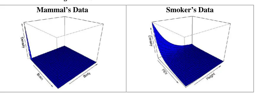
In this subsection we have applied the proposed multivariate Weibull distribution on two real data sets. The data set 1 contains information about body weight and brain weight of 84 mammals as reported by Ramsay and Schafer (1997). The second data set that we have used contains information about height and forced expiratory volume (FEV) of 655 smokers as reported by Rosner (1999). The bivariate Weibull distribution has been _tted on the data. The results are shown in the Table–3 below.

Table 3: Results of Fitted Distributions

Data Set ˆ _ˆ _LL _AIC

1 0.1783 0.1060 -996.338 1996.676

(12)

The bivariate histogram for two datasets given below

Figure 1: Bivariate Histograms of Two Data Sets

Mammal’s Data Smoker’s Data

We have further constructed the bivariate surface plots for two fits and are given in figure 2 below.

Figure 2: Surface Plots of Fitted Distributions

Mammal’s Data Smoker’s Data

We can see that the surface plot is close to bivariate histograms. Hence the bivariate Weibull distribution fits data reasonably well.

Conclusions and Recommendation

In this paper we have proposed a multivariate Weibull distribution and have studied some of its common properties. The distribution of multivariate concomitants of records for the proposed distribution has also been obtained. The distribution can be used to obtain the distribution of concomitants for any number of variables.

Acknowledgements

(13)

Deanship of Scientific Research at Umm Al–Qura University to Dr. Mashail Al–Sobhi (Grant Code: 15-SCI-3-3-0025).

The authors are also thankful to anonymous reviewers for helpful comments which improves quality of the paper.

References

1. Arnold, B. C., Castillo, E. and Sarabia, J. M. (2009). Multivariate Order Statistics via Multivariate Concomitants, Journal of Multivariate Analysis, 100, 946-951.

2. Ahsanullah, M. (1992). Record values of independent and identically distributed continuous random variables, Pak. J. Statist. Vol. 8(2), 9–34. 3. Ahsanullah, M. (1995). Record Statistics, Nova Science Publishers, USA.

4. Candler, K. N. (1952). The distribution and frequency of record values, J.

Roy. Statist. Soc., Series B, Vol. 14, 220–228.

5. Cordeiro, G. M., Ortega, E. M. M. and Nadarajah, S. (2010). The Kumaraswamy Weibull distribution with application to failure data,

Journal of Franklin Institute, 347, 1399-1429.

6. Eugene, N., Lee, C., Famoye, F. (2002). Beta-normal distribution and its applications. Communications in Statistics-Theory and Methods, 31, 497-512.

7. Filus, J.K. and Filus, L.Z. (2001). On some Bivariate Pseudonormal densities.

Pak. J. Statist. 17(1), 1-19.

8. Filus, J.K. and Filus, L.Z. (2006). On some new classes of Multivariate Probability Distribu- tions. Pak. J. Statist. 22(1), 21–42.

9. Famoye, F., Lee, C. and Olumolade, O. (2005). The Beta-Weibull Distribution,

Journal of Statistical Theory and Applications 4(2), 121-136.

10. Johnson, N. L., Kotz, S. and Balakrishnan, N. (1995). Continuous univariate

distributions, Vol. I & II, John Wiley and Sons, New York, USA.

11. Kotz, S., Balakrishnan, N. and Johnson, N.L. (2000). Continuous multivariate distributions, Vol. 1, Models and Applications, 2nd Edition,

John Wiley and Sons, New York, USA.

12. Mudholkar, G.S., Srivastava, D.K., (1993). Exponentiated Weibull family for analyzing bath- tub failure data. IEEE Trans. Reliability, 42, 299–302. 13. Nevzorov, V. B., (2001). Record: Mathematical Theory, Translations of

Mathematical Monographs, Vol. 194, American Mathematical Society.

14. Ramsey F.L. and Schafer D.W. (1997). The Statistical Sleuth, a course in methods of data analysis. Wadsworth.

(14)

16. Shahbaz, S. and Ahmad, M. (2009). Concomitants of order statistics for Bivariate Pseudo– Weibull distribution, World App. Sci. J., Vol. 6(10), 1409–1412.

17. Shahbaz, S. Shahbaz, M. Q., Ahsanullah, M. and Mohsin, M. (2011). On a New Class of Probability Distributions, App. Math. Letters, Vol. 24(5), 545–

552.

18. Shahbaz, S., Shahbaz, M. Q., Butt, N. S. and Ismail, M. (2014). The trivariate Pseudo Inverse Weibull distribution, Caspian J. App. Sci. Res., Vol. 3(9), 24–28.

19. Shahbaz, S., Shahbaz, M. Q., Rafiq, A. and Acu, A. M. (2012). On Trivariate Pseudo Weibull Distribution, Acta Uni. Apul., Vol. 31, 241–247.

20. Weibull, W. (1951). A statistical distribution function of wide applicability,