H.DAOUDI
Department of Mathematics.
Ibn Khladoun University, Tiaret, Algeria. Laboratory of Stochastic Process and Statistics. [email protected]
B.MECHAB
Department of Probability and Statistics. Djillali Liabs University, Algeria.
Laboratory of Stochastic Process and Statistics. [email protected]
Abstract
The main goal of this paper is to study the asymptotic normality of the estimate of the conditional distribution function of a scalar response variable Y given a hilbertian random variable X when the observations are quasi-associated. Our approach is based on the Doob’s technique. It is shown that, under the concentration property on small balls of the probability measure of the functional estimator and some regularity conditions, the kernel estimate of the conditional distribution function is asymptotically normally distributed. We performed out simulation experiments to examine the behavior of this asymptotic property over finite sample data.
Keywords: Conditional distribution function; probabilities of small balls; asymp-totic normality; nonparametric kernel estimation; quasi-associated data.
1. Introduction
In recent years, the functional estimate has attracted a lot of attention in the sta-tistical literature. Functional data arise in a variety of fields including econometrics, epidemiology, environmental science and many others.
The associated random variables play an important role in a wide variety of areas, in-cluding reliability theory, mathematical physics, multivariate statistical analysis, life sciences and in percolation theory. Many works were treated data under positive and negative dependant random variables, one can quote, Newman (1984) and Matula (1992). The concept of quasi-association is a special case of weak dependence intro-duced by Doukhan and Louhichi (1999) for real-valued stochastic processes. To the best of our knowledge, there is few papers dealing with the nonparametric estimation for quasi-associated random variables. We quote, Douge (2010) studied a limit theo-rem for quasi-associated hilbertian random variables, Attaoui and Ling (2016) studied asymptotic results of a nonparametric conditional cumulative distribution estimator in the single functional index modeling of time series data, Tabti and Ait Saidi (2018) studied the estimation and simulation of the conditional hazard function in the quasi-associated framework when the observations are linked via a functional single index structure, the asymptotic normality of this last estimator was studied by Daoudi et al. (2018). Mechab and Laksaci (2016) studied Nonparametric relative regression for associated random variables. Daoudi et al. (2019) studied the asymptotic normality of the nonparametric conditional density function estimate with functional variables for quasi-associated data
The main contribution of this work is the study of the asymptotic normality of the estimator of the conditional distribution function of Ferraty et al. (2006) in case of quasi-associated data. Note that, like all asymptotic statistics nonfunctional para-metric, our result is related to the phenomenon of concentration of the probability measure of the explanatory variable and regularity of the functional space of the model. we recall the definition of quasi-association:
Definition 1.1. A sequence (Xn)n∈N of real random vectors variables is said to be Quasi-Association (QA), if for any disjoint subsets I and J of N and all bounded Lipschitz functions f :R|I|d →
R and g :R|J|d→R satisfying
Cov(f(Xi, i∈I), g(Xj, j ∈J))≤Lip(f)Lip(g)
X
i∈I
X
j∈J d
X
k=1
d
X
l=1
Cov(Xik, Xjl)
where Xik denotes the kth component of Xi, Lip(f) = sup
x6=y
|f(x)−f(y)| ||x−y||1
with ||(x1, ..., xk)||1 =|x1|+· · ·+|xk|.
The paper is organized as follows: in the next section, we present our model. Section 3 is dedicated to fixing notations and hypotheses. We state our main results in Section 4. An application on simulated data is given to validate our theoretical result in Section 5. The auxiliary results and proofs are given in Section 6. We finalize the paper with a conclusion in Section 7.
2. The model
space with the norm k.k generated by an inner product< ., . >.
We consider the semi-metricd defined by∀x, x0 ∈ H, d(x, x0) =|< x−x0, α >|where α∈ H. In the following xwill be a fixed point in H.
We intend to estimate the conditional distribution function Fx(y) using n dependent observations (Xi, Yi)i∈N draw from a random variables with the same distribution with Z := (X, Y). To this aim, we introduce the kernel type estimator Fbx of Fx
defined by:
b
Fx(y) =
Pn
i=1K(h
−1
K d(x, Xi))H(h−H1(y−Yi))
Pn i=1K(h
−1
K d(x, Xi))
, ∀y∈R (1)
where K is the kernel, H is a given distribution function and hK = hK,n (resp. hH =hH,n) is a sequence of positive real numbers.
3. Notations and hypotheses
All along the paper, when no confusion will be possible, we will denote by C or/and C0 some strictly positive generic constants whose values are allowed to change. We assume that the random pair Zi = {(Xi, Yi), i ∈ N} is stationary quasi-associated processes.
Letλk the covariance coefficient defined as: λk =sups≥k
X
|i−j|≥s λi,j
where:
λi,j =
∞
X
k=1
∞
X
l=1
|cov(Xik, Xjl)|+
∞
X
k=1
|cov(Xik, Yj)|+
∞
X
l=1
|cov(Yi, Xjl)|+cov(Yi, Yj)|.
Xk
i denotes thekth component ofXi defined as Xik:=< Xi, ek >.
Forh >0, letB(x, h) :={x0 ∈ H/d(x0, x)< h} be the ball of centerx and radius h. To establish the asymptotic normality of the estimator Fbx, we need to include the
following assumptions:
(H1) P(d(x0, x) < hK) = φx(hK) > 0 and Moreover, there exists a function β(x, .) such that:
∀s∈[0,1], lim hK→0
φ(x, shK) φ(x, hK)
=β(x, s). .
(H2) For l ∈ {0,2}, the functions Φl(s) = E[∂ lFX(y)
∂yl −
∂lFx(y)
∂yl | d(x, X) = s] are differentiable at s= 0.
(H3) H is a cumulative distribution has derivative H0 such that: R
(H4) K is a kernel function and bounded continuous Lipschitz function such that: C1[0,1](.)< K(.)< C
0
1[0,1](.)
where1[0,1] is the indicator function on [0,1], and its derivativeK 0
is such that:
−∞< C < K0(t)< C0 <0 for 0≤t≤1.
(H5) The bandwidths (hK, hH) satisfied: (i) lim
n→∞hK = 0, nlim→∞hH = 0 and (ii) limn→∞(h
b2
H +h b1
K)
q
nφ(x, hK) = 0.
(H6) The sequence of random pairs (Xi, Xj), i∈Nis quasi-associated with covariance coefficient λk,k ∈N satisfying:
∃α >0,∃C > 0,such that λk ≤Ce−αk. (H7)
sup i6=j P
[(Xi, Xj)∈B(x, hK)×B(x, hK)] = Ψi,j >0
Ψi,j =maxi6=j{P(d(x, Xi))< hK,P(d(x, Xj))< hK)}=O(φ2x(hK)).
Comments on the hypotheses
Assumption (H1) is the concentration property of the explanatory variable in small balls. The function β(x, .) plays a fundamental role in all asymptotic, in particular for the variance term. The condition (H2) is used to control the regularity of the functional space of our model and these are needed to evaluate the bias term of the convergence rates. The hypotheses (H3) and (H4) are technical conditions on the cumulative function H and the kernels K, H0 and K0. Assumption (H5) is also classical in the functional estimation in finite or infinite dimension spaces, in particular, is used to eliminate the term bias in the result of asymptotic normality. The hypothesis (H6) is a structural condition used for the quasi-associated data. To establish the asymptotic normality of our model under quasi-association, we need the assumption (H7), which describes the asymptotic behavior of the joint distribution of the couple (Xi, Xj).
4. Main Results: Asymptotic Normality
Theorem 4.1. Under hypotheses (H1)-(H7), as n goes to infinity, we have:
s
nφ(x, hK) σ2(x)
b
Fx(y)−Fx(y)−→ ND (0,1) n → ∞
where
σ2(x) = C2F
x(y)(1−Fx(y)) C2
1
Z
with
Cj =K(1)−
Z 1
0
(Kj)0(s)β(x, s)ds, for j = 1,2.
Proof of Theorem 4.1. The proof of this theorem is based on the following decom-position and the lemmas bellow:
b
Fx(y)−Fx(y) = Fb x
N(y)−Fx(y)FbDx(y) b
Fx D(y)
= 1
b
Fx D(y)
{FbNx(y)−E(FbNx(y))
+ E(FbNx(y))−FNx(y))}
− 1
b
Fx D(y)
n
Fx(y)(FbDx(y)−1) o
where
b
FNx(y) = 1 nE(K1(x))
n
X
i=1
Ki(x)Hi(y) and
b
FDx = 1 nE(K1(x))
n
X
i=1
Ki(x), with
Ki(x) =K h−K1d(x, Xi) and Hi(y) = H h−H1(y−Yi).
Finally, to state the asymptotic normality of Fx(y), we show that the numerator suitably normalized is asymptotically normally distributed (with law N(0, σ2(x))) and that the denominator converges in probability to 1.
Then, the proof of Theorem 4.1 can be deduced from the following lemmas:
Lemma 4.1. Under the hypotheses of Theorem 4.1, as n goes to infinity, we have:
p
nφ(x, hK)
b
FNx(y)−E(FbNx(y))
D
−→ N(0, σ2(x)).
Lemma 4.2. (See, (Laksaci and Mechab, 2014)). Under the hypotheses (H1)-(H5), we have:
E(FbNx(y))−FNx(y) =BHF(x, y)h2H +BKF(x, y)hK+o(h2H) +o(hK)
where
BHF(x, y) = 1 2
∂2Fx(y) ∂y2
Z
t2H0(t)dt and
BKF(x, y) = hKΦ00(0)
C0
C1
Lemma 4.3. Under the hypothesis (H1)-(H7), as n goes to infinity, we have:
p
nφ(x, hK)
Fx(y)(FbDx(y)−1)
→0 in probability. Lemma 4.4. Under hypotheses of Theorem 4.1, we have
X
n∈N
P
b
FDx(y)<1/2<∞.
5. Application on simulated data
We aim to evaluate, on a finite sample, performances of the asymptotic normality of the conditional distribution on simulated data. In particular, our main purpose is to show how we can implement easily and quickly this estimator in practice. Of course, the applicability of our asymptotic normality result requires a practical estimation of the asymptotic bias and variance.
The main purpose of this section is to test the effectiveness of the two asymptotic normality results. For this purpose, we consider the functional nonparametric model as follows:
Y =r(x) + where ∼ N(0,1)
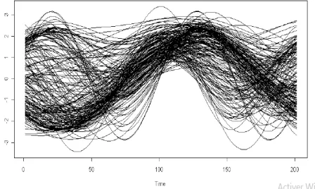
We are interested in functional data derived from a mixture of two Gaussian stochastic processes Z1(t) and Z2(t) over an interval [-1,1] defined by:
Z1(t) = p
−2log(U)cos(2π(1−W)t), Z2(t) = p
−2log(1−U)sin(2πW t) where U and W are random variables distributed uniformly over the interval [0,1]. The explanatory functional variables are quasi-associated are constructed by:
X(t) = Z1(t) +Z2(t)
We generate a sample of size 200 {Xi(t)}i=1,...,200 of X(t), and we observe each
vari-able Xi on (tj)j=1,...,100 ∈[−1,1]).
The curves obtained are plotted in Figure1: On the other hand, fori= 1, ..., n= 200,
the scalar response Yi is computed by considering the following operator: r(x) =
Z 1
0
dt 1+ |x(t)|
Recall that, the conditional distribution of Y given X = x corresponding to this model is explicitly given by the law of i shifted by r(x). Then, the corresponding conditional density fx(y) is:
fx(y) = 1
2π exp(− 1
2(y−r(x))
2
Elsewhere, as it is well-known in FDA, the choice of the metric and the smoothing parameters have crucial roles in the computational issues. To optimize these choices in this illustration, we use firstly the cross-validation procedure method for choosing smoothing parameters, secondly regarding the shape of the curvesXi , it is clear that the PCA-type semi-metric (see Benhenni et al. 2007), is well-adapted to this kind of data. Then, we point out that, we opted for a quadratic kernel which is supported within (0,1) and taken K =H0.
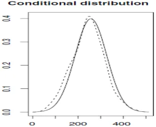
Figure 2: The asymptotic distribution of the conditional distribution function
The obtained results are shown in figure2. It appears clearly that, asymptotic distri-butions have good behaviors with respect to the standard normal distribution. This conclusion is confirmed by the Kolmogorov-Smirnov test which, for n = m = 200 , gives 0.80 as aP value for the first model and 0.69 for the second one.
6. Auxiliary results and proofs
First of all, we state the following lemmas.
Lemma 6.1. (See, Douge (2010)). Let (Xn)n∈N be a quasi-associated sequence of random variables with values in H. Let f ∈BL(H|I|)∩
L∞ and g ∈BL(H|J|)∩L∞, for some finite disjoint subsets I, J ⊂N. Then
Cov(f(Xi, i∈I), g(Xj, j ∈J))≤Lip(f)Lip(g)
X
i∈I
X
j∈J
∞
X
k=1
∞
X
l=1
Cov(Xik, Xjl)
where (BL(Hu;u >0) is the set of bounded Lipschitz functions f :Hu →
is the set of bounded functions.
Lemma 6.2. (See, Kallabis and Nemann (2006)). Let X1, ..., Xn the real random variables such that E(Xj) = 0 and P(| Xj |≤ M) = 1 for allj = 1, ..., n and some M <∞, Let σ2
n =V ar(
Pn
i=1∆i).
Assume, furthermore, that there exist K < ∞ and β > 0 such that, for all u-uplets (s1, ..., su)∈Nu, (t1, ..., tv)∈Nv with 1≤s1 ≤ · · · ≤su ≤t1 ≤ · · · ≤tv ≤n.
The following inequality is fulfilled:
|cov(Xs1...Xsu, Xt1...Xtv)|≤K
2Mu+v−2ve−β(t1−su).
Then,
P(| n
X
j=1
Xj |> t)≤exp{−
t2/2
An+B
1/3
n t5/2
}
for some
An ≤σ2n and
Bn = (
16nK2
9An(1−e−β)∨1)
2(K ∨M) 1−e−β .
6.1 Proof of lemma 4.1
We denote
Zni(x, y) =
p
φ(x, hK)
√
nE(K1)
(Γi(x, y)−EΓi(x, y))
where
Γi(x, y) =K(h−K1d(x, Xi))Hi(y)−E[K1H1],1≤i≤n
and
Sn:= n
X
i=1
Zni(x, y) (2)
Therefore,
Sn =
p
nφ(x, hK)(FbN(x, y)−E(FbN(x, y)). Thus, our claimed result is, now:
Sn → N(0, σ2(x)).
To do that, we use the basic technique of Doob (1959). Indeed, we consider p = pn and q =qn two sequences of natural numbers tending to infinity, such that
p=O(pnφ(x, hK)), q =o(p) and we split Sn into
Sn =Tn+Tn0 +ξk with Tn =Pkj=1ηj and Tn0 =
Pk
where
ηj =
X
i∈IJ
Zni(x, y), ξj =
X
i∈IJ
Zni(x, y), ζk =
X
i=k(p+q)+1
Zni(x, y)
with
Ij = (j−1)(p+q) + 1, ...,(j−1)(p+q) +p, Jj = (j−1)(p+q) +p+ 1, ..., j(p+q).
Observe that, for k = p+nq, (where [.] stands for the integral part), we havekqn → 0 and kpn →1,nq →0 , which imply that np →0 as n → ∞.
Now, our asymptotic result is based on:
E(Tn0)
2+
E(ζn)2 →0 (3) and
Tn → N(0,1). (4)
Proof of (3).
By stationarity, we get
E(Tn0)
2 =kV ar(ζ 1) + 2
X
1≤i<j≤k
|Cov(ζi, ζj)| (5)
and
kV ar(ζ1)≤qkV ar(Zn1(x, y)) + 2k X
1≤i<j≤k
Cov(Zni(x, y), Znj(x, y)) (6)
by the fact that kqn →0. We obtain
qkV ar(Zn1(x, y)) = φ(x, hK)qk 1 n(E(K1))2
V ar(Γ1(x, y))
= O(kq
n )→0, as n→ ∞. On the other hand, we have
k X
1≤i<j≤k
|Cov(Zni(x, y), Znj(x, y))|=
kφ(x, hK) n(E(K1))2
X
1≤i<j≤k
Cov(Zni(x, y), Znj(x, y))
we obtain,
X
1≤i<j≤k
|Cov(Zni(x, y), Znj(x, y))|=o(qφ(x, hK)). Then
k X
1≤i<j≤k
|Cov(Zni(x, y), Znj(x, y))|=O( kq
From (5)-(7), we obtain
kV ar(ξi)→0, asn → ∞. (8) We use the stationarity, to evaluate the second term in the right-hand side of (4)
X
1≤i<j≤k
|Cov(ξni, ξnj)| =
X
1≤i<j≤k
(k−l)|Cov(ξni, ξnj)|
≤ k X
1≤i<j≤k
|Cov(ξni, ξnj)|
≤
k−1 X
l=1
X
(i,j)∈J×Jl+1
Cov(Zni(x, y), Znj(x, y))
It is clear that, for all (i, j)∈Ji×Jj, we have |i−j| ≥p+ 1 > p, then
X
1≤i<j≤k
|Cov(ξni, ξnj)| ≤ kCφ(x, hK)(h
−1
K Lip(K) +h
−1
H Lip(H))
2
n(E[K1)2
p
X
i=1
v
X
j=2p+q+1,|i−j|>p λi,j
≤ Ckpφ(x, hK)(h
−1
K Lip(K) +h
−1
H Lip(H))2 n(E[K1)2
λp
≤ Ckp(h
−1
K Lip(K) +h
−1
H Lip(H))2 nφ(x, hK)
e−αp
≤ Ckp
nh2
Hφ3(x, hK)
e−αp→0.
Finally, by combining this last result and (7). We can write
E(T10)
2 →0 as n→ ∞. (9)
Moreover
E(ζk)2 ≤ (n−k(p+q))V ar(Zn1(x, y)) + 2 X
1≤i<j≤k
|Cov(Zni(x, y), Znj(x, y))|
≤ pV ar(Zn1(x, y)) + 2 X
1≤i<j≤k
|Cov(Zni(x, y), Znj(x, y))|
≤ pφ(x, hK)
nE(K1)2
V ar(Zn1(x, y)) +
Cφ(x, hK) nE(K1)2
X
1≤i<j≤k
|Cov(Zni(x, y), Znj(x, y))|
| {z }
o(1)
≤ Cp
n +o(1). Then,
The proof of convergence in (6) is based in the following two results
|E(eitPkj=1ηj)−
k
Y
j=1
E(eitηj)|→0 (10)
and
kV ar(η1)→σ2(x), kE(η121η1>σ(x))→0. (11)
Proof of (10).
|E(eitPkj=1ηj)−
k
Y
j=1
E(eitηj)| ≤ |E(eit
Pk
j=1ηj)−E(eit
Pk−1
j=1ηj)E(eitηj)|
+ |E(eitPkj=1−1ηj)−
k−1 Y
j=1
E(eitηj)|
= |Cov(eitPjk=1−1ηj, eitηk)|+| E(eit
Pk−1
j=1ηj)
−
k−1 Y
j=1
E(eitηj)| (12)
and successively, we have
|E(eitPkj=1ηj)−
k
Y
j=1
E(eitηj)|≤|Cov(eit
Pk−1
j=1ηj, eitηk)|+|Cov(eit
Pk−2
j=1ηk−1, eitηj)|
+· · ·+|Cov(eitη2, eitη1)|. (13)
Once again we apply Lemma 6.2, to write
|Cov(eitη2, eitη1)|≤C(h−1
K Lip(K) +h
−1
H Lip(H))
2 φ(x, hK) n(E[K1)2
X
i∈I1
X
j∈I2
λi,j.
Applying this inequality to each term on the right-hand side of (13). We obtain
|E(eitPkj=1ηj)−
k
Y
j=1
E(eitηj)|≤C(h−K1Lip(K) +h
−1
H Lip(H))
2φ(x, hK) n(EK1)2
×
X
i∈I1
X
j∈I2
λi,j+
X
i∈I1∪I2
X
j∈I3
λi,j+· · ·+
X
i∈I1∪···∪Ik−1
X
j∈Ik λi,j
.
Observe that for every 2 ≤ l ≤ k−1,(i, j) ∈ Il∗Il+1, we have |i−j| ≥ q+ 1 > q,
then
X
i∈I1∪···∪Ik−1
X
j∈Ik
Therefore, inequality (12) becomes
|E(eitPkj=1ηj)−
k
Y
j=1
E(eitηj)| = Ct2(h−K1Lip(K) +h
−1
H Lip(H))
2 φ(x, hK) n(E[K1])2
kpλq
= Ct2(h−K1Lip(K) +h−H1Lip(H))2φ(x, hK) (E[K1])2
kpe−αq = Ct2(h−K1Lip(K) +h−H1Lip(H))2 1
nφ(x, hK) kpλq
= Ct2 kp
nh2
Hφ3(x, hK)
λq →0. Proof of (11).
By the same arguments used in 5, we have lim
n→∞kV ar(η1) = nlim→∞kpV ar(Zn1(x, y))
= lim n→∞
φ(x, hK) n(EK1)2
V ar(Γ1(x, y))
So, by using the same arguments as those used by (Ferraty and Vieu, 2007), we get 1
φ(x, hK)E
(K12)→K12−
Z 1
0
(K2)0(s)β(x, s)ds+o(1) E(K12H12)
E(K12)
→Fx(y)(1−Fx(y))
Z
H02(t)dt E(K12H12)
E(K12)
→Fx(y)(1−Fx(y)) which imply that
φ(x, hK) n(EK1)2
V ar(Γ1(x, y))→σ2(x).
Hence
kV ar(η1)→σ2(x).
For the second part of (11), we use the fact that:
|η1 |≤Cp|Zn1(x, y)|≤
Cp
p
nφ(x, hK) and by Tchebychev’s inequality we get:
kE(η121η1>σ(x)) ≤
Cp2k
nφ(x, hK)P
(η1 > σ(x))
≤ Cp
2k
nφ(x, hK)
V ar(η1)
2σ2(x)
= O
p2
nφ(x, hK)
6.2 Proof of lemma 4.3
We have
|FbDx(y)−EFbDx(y)|=
1 nE[K1]
n
X
i=1
∆i
where
∆i =K(h−K1d(x, Xi))−E[K1],1≤i≤n
clearly we haveE(∆i) = 0 and Moreover, we can write:
k∆i k∞ 1 ≤2C kK k∞
and
Lip(∆i)≤Ch−K1Lip(K).
Now, to apply lemma 6.2, we have to evaluate the variance term V ar(Pn
i=1∆i) and
the covariance term cov(∆s1...∆su,∆t1...∆tv), for all (s1, ..., su) ∈ N
u,(t
1, ..., tv) ∈ Nv with 1≤s1 ≤ · · · ≤su ≤t1 ≤ · · · ≤tv ≤n.
Firstly, for the covariance term, we consider the following cases: Ift1 =su. By using the fact that E[|K1 |] =O(φ(x, hK)) we have:
|Cov(∆s1...∆su,∆t1...∆tv)| ≤
C nE[K1]
u+v
E|∆i |u+v
≤
C kK k∞
nE[K1] u+v
E[|K1 |]
≤ φ(x, hK)
C nφ(x, hK)
u+v
If t1 > su, we use the quasi-association, under (H7), we get :
|Cov(∆s1...∆su,∆t1...∆tv)| ≤
Lip(K) nhKE[K1]
2
×
C nE[K1]
u+v−2 u X
i=1
v
X
j=1
λsi,tj
≤ h−K1Lip(K)2
C nE[K1]
u+v
vλt1−su
≤ h−K1Lip(K)2
C φ(x, hK)
u+v
ve−α(t1−su).
(14) On the other hand, by (H7) we have:
|Cov(∆s1...∆su,∆t1...∆tv)|≤
CkK k∞
n[K1]
u+v−2
(|E[∆su,∆t1]|+E|∆su |E|∆t1 |
≤
CkK k∞
nE[K1]
u+v−2
C nE[K1]
2
× (supi6=jP (Xi, Xj)∈B(x, hK)×B(x, hK) +P(X1 ∈B(x, hK))
2
≤
C φ(x, hK)
u+v
(φ(x, hK))2.
(15) Furthermore, taking a γ−power of (14), (1−γ)−power of (15), with 1 = 4< γ < 1 = 2, we obtain an upper-bound of the tree terms as follows: for 1 ≤ s1 ≤ · · · ≤
su ≤t1 ≤ · · · ≤tv ≤n
|cov(∆s1...∆su,∆t1...∆tv)|≤φ(x, hK)
C nφ(x, hK)
u+v
. Secondly, for the variance term V ar(Pn
i=1∆i), we put, for all 1≤i≤n,
|V ar(∆s1...∆su,∆t1...∆tv)| =
1 nE[K1]
2 n
X
i=1
n
X
j=1
Cov(Ki, Kj)
=
1 nE[K1]
2
V ar(K1)
+
1 nE[K1]
2 n
X
i=1
n
X
j=1,i6=j
Cov(Ki, Kj)
(16) for the first term,
V ar(K1) =E K12
−(E(K1))2
then,
E[K12] =O(φ(x, hK)). It follows that:
1 nE[K1]
2
For this, we need the following decomposition: n
X
i=1
n
X
j=1,i6=j
Cov(Ki, Kj) = n
X
i=1
n
X
j=1,0<|i−j|≤mn
Cov(Ki, Kj)
| {z }
I
+ n
X
i=1
n
X
j=1,|i−j|>mn
Cov(Ki, Kj)
| {z }
II
where (mn) is a sequence of positive integer which goes to infinity asn → ∞. From Assumptions (H1), (H4) and (H8), we have, fori6=j
I ≤ nmn maxi6=j |E(KiKj)|+(E(K1))2
≤ Cnmn φ2(x, hK) +φ2(x, hK)
≤ Cnmn φ2(x, hK)
.
(18) Since the kernels K is bounded and Lipschitzian, we get
II ≤ (h−K1Lip(K))2 u
X
i=1
v
X
j=1|i−j|>mn λi,j
≤ C(h−K1Lip(K))2 u
X
i=1
v
X
j=1|i−j|>mn λi,j
≤ Cn(h−K1Lip(K))2λmn
≤ Cn(h−K1Lip(K))2e−αmn.
(19) Then, by (18) and (19), we get
n
X
j=1,i6=j
Cov(Ki, Kj)≤C
nmn(φ2(x, hK)) +n h−K1Lip(K)
2
e−αmn
by choosing
mn= log
(h−K1Lip(K))2 αφ2(x, h
K)
we get
1 φ(x, hK)
n
X
j=1,i6=j
Finally, by combining results (16), (17) and (20), we get:
V ar n
X
i=1
∆i
!
=O
1 nφ(x, hK)
.
6.3 Proof of lemma 4.4
We have
P{|FbDx(y)| ≤1/2} ≤ P{|FbDx(y)−1|>1/2}
≤ P{|FbDx(y)−EFbDx(y)|>1/2}
we deduce that
X
n∈N
P
b
FDx(y)<1/2<∞.
7. Conclusion
In this paper, we established the asymptotic normality property of the kernel estimate of the conditional distribution function in quasi-associated data framework. Our the-oretical and practical studies confirm that our kernel estimator has good asymptotic properties.
References
1. Attaoui, S., Laksaci, A. and Ould-Sa¨ıd, E. (2015). Asymptotic Results for an estimator of the Regression Function for Quasi-Associated Pro-cesses. Functional Statistics and Applications, Contributions to Statistics 10.1007/978-3-319-22476-3-1.
2. Daoudi, H. and B. Mechab. (2019). Rate of pointwise consistency for non-parametric of the conditional distribution function estimate with func-tional variables for quasi-associated data, Statistics, optimization and information computing, Accepted:27/07/2019.
3. Daoudi, H., Mechab, B. and Elmezouar, C.Z. (2018). Asymptotic Normality of a Conditional Hazard Func-tion Estimate in the Single Index for Quasi-Associated Data, Communication in Statistics Theory and Methods. https://www.tandfonline.com/doi/full/10.1080/03610926.2018.1549248. 4. Daoudi, H., Mechab, B., Benaissa, S., and Rabhi., A. (2019). Asymp-totic normality of the nonparametric conditional density function esti-mate with functional variables for the quasi-associated data, Interna-tional Journal of Statistics and Economics 20(3), 94-106.
6. Doukhan, P. and Louhichi, S. (1999). A new weak dependence condition and applications to moment inequalities, Stoch. Proc. Appl 84, 313-342. 7. Ezzahrioui, M. and Ould-Sa¨ıd, E. (2008). Asymptotic Results of a Non-parametric Conditional Quantile Estimator for Functional Time Series, Communication in Statistics Theory and Methods 37(17), 2735-2759. 8. Ferraty, F. Mas, A. and Vieu, P., (2007). Advances in nonparametric
re-gression for functional variables. Aust. and New Zeal. J. of Statist 49, 1-20.
9. Kallabis, R. S. and Neumann, M. H. (2006). An exponential inequality under weak dependence, Bernoulli 12, 333-350.
10. Laksaci, A. and B. Mechab. (2014). Conditional hazard estimate for func-tional random fields. Journal of Statistical Theory and Practice 8, 192-200.
11. Mechab, W. and Laksaci, A. ( 2016). Nonparametric relative regression for associated random variables, Metron 74, 75-97.