The Transmuted Geometric-Weibull distribution: Properties, Characterizations and Regression Models

Properties, Characterizations and Regression Models

Zohdy M. Nofal

Department of Statistics, Mathematics and Insurance, Benha University, Egypt [email protected]

Yehia M. El Gebaly

Department of Statistics, Mathematics and Insurance, Benha University, Egypt [email protected]

Emrah Altun

Department of Statistics,Hacettepe University, Turkey [email protected]

Morad Alizadeh

Department of Statistics, Persian Gulf University, Bushehr, Iran [email protected]

Nadeem Shafique Butt

Department of Family and Community Medicine, Faculy of Medicine King Abdulaziz University, Kingdom of Saudi Arabia

[email protected]

Abstract

We propose a new lifetime model called the transmuted geometric-Weibull distribution. Some of its structural properties including ordinary and incomplete moments, quantile and generating functions, probability weighted moments, Rényi and q-entropies and order statistics are derived. The maximum likelihood method is discussed to estimate the model parameters by means of Monte Carlo simulation study. A new location-scale regression model is introduced based on the proposed distribution. The new distribution is applied to two real data sets to illustrate its flexibility. Empirical results indicate that proposed distribution can be alternative model to other lifetime models available in the literature for modeling real data in many areas.

Keywords: Goodness of fit, Lifetime data, Maximum likelihood, Moment, Order statistic, Regression model.

1. Introduction

generalization of the Weibull distribution studied in the literature includes, but are not limited to, exponentiated Weibull (Mudholkar and Srivastava, 1993; Mudholkaret al. 1995; Mudholkar, Srivastava et al. 1996), additive Weibull (Xie and Lai, 1995), Marshall-Olkin extended Weibull (Ghitany et al. 2005), beta Weibull (Famoye et al. 2005), modified Weibull (Sarhan and Zaindin, 2009), beta modified Weibull (Silva et al. 2010), transmuted Weibull (Aryal and Tsokos, 2011), extended Weibull (Xie et al. 2002), modifiedWeibull (Lai et al. 2003), KumaraswamyWeibull (Cordeiro et al. 2010), Kumaraswamy modified Weibull (Cordeiro et al. 2012), Kumaraswamy inverse Weibull (Shahbaz et al. 2012), exponentiated generalized Weibull (Cordeiro et al. 2013), McDonald modified Weibull (Merovci and Elbatal, 2013), beta inverse Weibull (Hanook et al. 2013), transmuted exponentiated generalized Weibull (Yousof et al., 2015), McDonald Weibull (Cordeiro et al. 2014), gamma Weibull (Provost et al, 2011), transmuted modified Weibull (Khan and King, 2013), beta Weibull (Lee et al. 2007), generalized transmuted Weibull (Nofal et al, 2017), transmuted additiveWeibull (Elbatal and Aryal, 2013), exponentiated generalized modified Weibull (Aryal and Elbatl, 2015), transmuted exponentiated additive Weibull (Nofal et al. 2016), Marshall Olkin additive Weibull (Afify et al. 2016), Kumaraswamy transmuted exponentiated additive Weibull (Nofal et al, 2016) distributions and the Topp-Leone Generated Weibull distribution (Aryal et al, 2016)

Let 𝑝(𝑡) be the probability density function (pdf) of a random variable 𝑇 ∈ 𝑎, 𝑏] for −∞ < 𝑎 < 𝑏 <∞ and let 𝑊[𝐺(𝑥)] be a function of the cumulative distribution function (cdf) of a random variable 𝑋 such that 𝑊[𝐺(𝑥)] satisfies the following conditions:

(

(𝑖) 𝑊[𝐺(𝑥)] ∈ 𝑎, 𝑏],

(𝑖𝑖) 𝑊[𝐺(𝑥)]isdifferentiableandmonotonicallynon − decreasing, and (𝑖𝑖𝑖) 𝑊[𝐺(𝑥)] → 𝑎 as 𝑥 → −∞ and 𝑊[𝐺(𝑥)] → 𝑏 as 𝑥 →∞.

(1)

Recently, Alzaatreh et al. (2013) defined the T-X family of distributions by

𝐹(𝑥) = ∫_𝑎𝑊[𝐺(𝑥)] 𝑝(𝑡) 𝑑𝑡, (2)

where 𝑊[𝐺(𝑥)] satisfies conditions (1). The pdf corresponding to (2) is given by 𝑓(𝑥) = {𝑑

𝑑𝑥 𝑊[𝐺(𝑥)]} 𝑝{ 𝑊[𝐺(𝑥)]}. (3)

According to Afify et al. (2016) the cdf of the TG-G family is given by

𝐹_{𝑇𝐺−𝐺}(𝑥) = ∫

𝜃 𝐺(𝑥;ϕ) 1+(𝜃−1)𝐺(𝑥;ϕ)

0

(1 + 𝜆 − 2 𝜆 𝑡) 𝑑𝑡

= 𝜃𝐺(𝑥; ϕ)

1 + (𝜃 − 1)𝐺(𝑥; ϕ){1 +

𝜆𝐺(𝑥; ϕ)

1 + (𝜃 − 1)𝐺(𝑥; ϕ)},

where 𝐺(𝑥; ϕ) and 𝜃 > 0, |𝜆| ≤ 1 are two additional shape parameters. The TG-G is a wider class of continuous distributions. It includes the transmuted-G family of distributions and geometric-G. Concider the cdf of the Weibull (W) distribution,

𝐺(𝑥; 𝛼, 𝛽) = 1 − e−(𝛼𝑥)𝛽 , Then using 𝐹𝑇𝐺−𝐺(𝑥) we get

𝐹(𝑥) =

𝜃(1−e−(𝛼𝑥)𝛽 ₎

1+(𝜃−1)(1−e−(𝛼𝑥)𝛽 ₎{1 +

𝜆e−(𝛼𝑥)𝛽

The pdf corresponding of (4) is given by

𝑓(𝑥) =𝜃𝛽𝛼𝛽𝑥𝛽−1

e(𝛼𝑥)𝛽 [1 + (𝜃 − 1) (1 − e

−(𝛼𝑥)𝛽_)]−2_{[1 + 𝜆 −} 2𝜆𝜃(1−e−(𝛼𝑥)𝛽)

1+(𝜃−1)(1−e−(𝛼𝑥)𝛽₎]. (5)

For 𝜆 = 0 we obtain geometric-W (GW) distribution. We denote by 𝑋~TG-W(𝜆, 𝜃, 𝛼, 𝛽) a random variable having density function (5).

The rest of the paper is organized as follows: In Section 2, some mathematical properties of the TGW are obtained such as mixture representation, quantile function, moments, order statistics and reliability estimation. Section 4 is devoted to characterizations of the proposed distribution and in Section 5 estimation of model parameters by the maximum likelihood method is presented. In Section 5, brief Monte-Carlo simulation study is performed to estimate model parameters with maximum likelihood estimators (MLE). The log-transmuted geometric-Weibull regression model is defined in Section 6. Section 7 is devoted to applications to illustrate the flexibility of the proposed distribution in many fields such as univariate data fitting and survival analysis. Finally, some concluding remarks are given in Section 8.

2. Mathematical Properties

In this section some mathematical properties of the TWG distribution is discussed.

2.1. Survival and Hazard Functions

Central role is played in the reliability theory by the quotient of the pdf and survival function. We obtain the survival function corresponding to (4) as

𝑆(𝑥) = 1 − 𝜃 (1 − e

−(𝛼𝑥)𝛽₎

1 + (𝜃 − 1)(1 − e−(𝛼𝑥)𝛽 ){1 +

𝜆e−(𝛼𝑥)𝛽

1 + (𝜃 − 1)(1 − e−(𝛼𝑥)𝛽 )}

In reliability studies, the hazard rate function (hrf) is an important characteristic and fundamental to the design of safe systems in a wide variety of applications. Therefore, we discuss these properties of the TGW distribution. The hrf of X takes the form

ℎ(𝑥) = 𝜃𝛽𝛼

𝛽_𝑥𝛽−1

e(𝛼𝑥)𝛽 [1 + (𝜃 − 1) (1 − e

−(𝛼𝑥)𝛽

)]−2[1 + 𝜆 − 2𝜆𝜃 (1 − e

−(𝛼𝑥)𝛽₎

1 + (𝜃 − 1)(1 − e−(𝛼𝑥)𝛽

)]

× {1 − 𝜃 (1 − e

−(𝛼𝑥)𝛽₎

1 + (𝜃 − 1)(1 − e−(𝛼𝑥)𝛽

){1 +

𝜆e−(𝛼𝑥)𝛽

1 + (𝜃 − 1)(1 − e−(𝛼𝑥)𝛽

)}}

−1

.

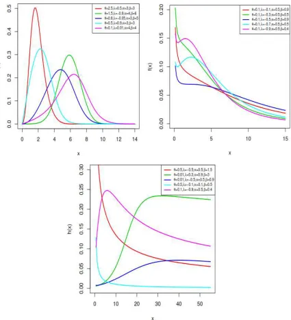
Figure 1. Plots of pdf and hrf of the TGW distribution for the selected parameter values.

2.2. Asymptotics

Proposition 2.1 The asymptotics of TGW distribution from cdf, pdf and hrf as 𝑥 → 0 are given by

𝐹(𝑥): 𝜃(1 + 𝜆)(𝛼 𝑥)𝛽, 𝑓(𝑥): 𝜃 𝛽(1 + 𝜆)𝛼𝛽 _𝑥𝛽−1_,

Proposition 2.2 The asymptotics of TGW distribution from cdf, pdf and hrf as 𝑥 →∞ are given by

1 − 𝐹(𝑥): e−(𝛼 𝑥)𝛽, 𝑓(𝑥): 𝛽 𝛼𝛽 _𝑥𝛽−1 _e−(𝛼 𝑥)𝛽_,

ℎ(𝑥): 𝛽 𝛼𝛽 𝑥𝛽−1.

These equations show the effect of parameters on tails of TGW distribution.

2.3. Mixture Representation

In this section, we provide a very useful representation for the TG-W density. The pdf in (5) can be rewritten as

𝑓(𝑥) =𝜃(1+𝜆) 𝛽𝛼𝛽𝑥𝛽−1 e−(𝛼𝑥)𝛽

[1+(𝜃−1)(1−e−(𝛼𝑥)𝛽_)]2 −

2𝜆𝜃2 𝛽𝛼𝛽𝑥𝛽−1 e−(𝛼𝑥)𝛽 (1−e−(𝛼𝑥)𝛽)

[1+(𝜃−1)(1−e−(𝛼𝑥)𝛽_)]3 (6)

Then, the pdf in (6) can be rewritten as

𝑓(𝑥) = (1 + 𝜆)𝜃 𝛽𝛼𝛽𝑥𝛽−1 e−(𝛼𝑥)𝛽∑∞_𝑘=0 (𝜃 − 1)𝑘 (−2

𝑘 ) (1 − e

−(𝛼𝑥)𝛽₎𝑘

−2 𝜆𝜃2 𝛽𝛼𝛽𝑥𝛽−1 e−(𝛼𝑥)𝛽∑∞_𝑘=0 (𝜃 − 1)𝑘 (−3

𝑘 ) (1 − e

−(𝛼𝑥)𝛽₎𝑘+1_.

(7)

the pdf (7) can be expressed as a mixture of exp-W density

𝑓(𝑥) = ∑∞_𝑘=0[𝑎_𝑘 𝜋_𝑘+1(𝑥) − 𝑏_𝑘 𝜋_𝑘+2(𝑥)]. (8)

But

(−2

𝑘 ) (= (−1)𝑘 (𝑘 + 1) and ( −3

𝑘 ) =

(−1)𝑘 _{(𝑘 + 1)(𝑘 + 2)}

2 ,

where

𝜋_𝛿(𝑥) = 𝛿𝛽𝛼𝛽_𝑥𝛽−1 _e−(𝛼𝑥)𝛽 _{(1 − e}−(𝛼𝑥)𝛽₎𝛿−1

is the exp-G pdf with power parameter 𝛿 > 0,

𝑎𝑘 = 𝜃(1 + 𝜆) (1 − 𝜃)𝑘 and 𝑏𝑘 = 𝜆 𝜃2 (𝑘 + 1) (1 − 𝜃)𝑘

Thus, several mathematical properties of the TG-W density can be obtained simply from those properties of the exp-W density. Equation (8) is the main result of this section.

The cdf of the TG-W distribution can also be expressed as a mixture of exp-W densities. By integrating (8), we obtain the same mixture representation

𝐹(𝑥) = ∑

𝑘=0

∞

[𝑎_𝑘Π_𝑘+1(𝑥) − 𝑏𝑘Π𝑘+2(𝑥)],

2.4. Quantile Function

The quantile function (qf ) of 𝑋, where 𝑋:TG-W(𝜆, 𝜃, 𝛼, 𝛽), is obtained by inverting (3) to obtain 𝑄(𝑢) = 𝐹−1(𝑢) as

𝑄(𝑢) =1 𝛼[ln [

2𝑢(1 − 𝜃)2_{+ 2𝜃(1 + 𝜆) − 2𝜃}2

2𝑢𝜃(1 − 𝜃) + 𝜃(1 + 𝜆) − 2𝜃2_{+ 𝜃√(1 + 𝜆)}2_{− 4𝑢𝜆}]]

1 𝛽

, for 𝜆 ≠ 0, 𝑢 ∈ (0,1).

For 𝜆 = 0 , we have

𝑄(𝑢) = 1 𝛼[ln [

𝑢(1 − 𝜃)2+ 𝜃 − 𝜃2 𝑢𝜃(1 − 𝜃) + 𝜃 − 𝜃2]]

1 𝛽

Simulating the TG-W random variable is straightforward. If 𝑈 is a uniform variate on the unit interval (0,1), then the random variable 𝑋 = 𝑄(𝑈) follows 6.

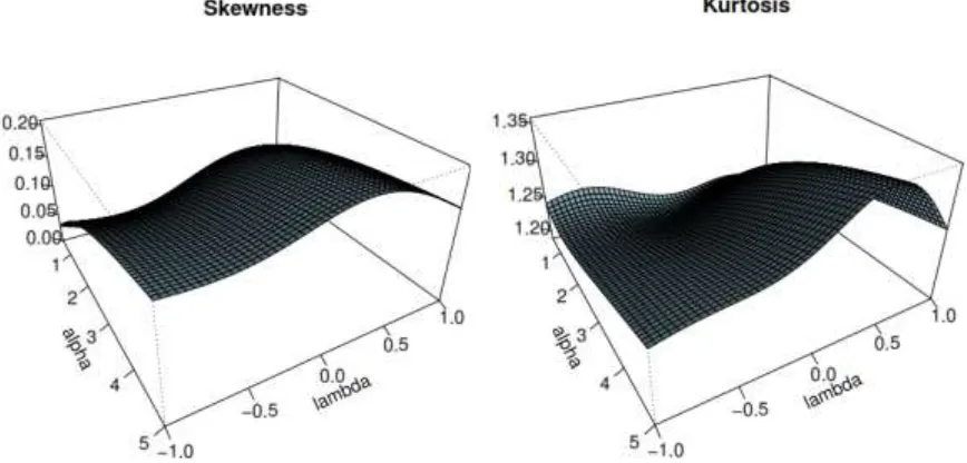
The effects of the shape parameters on the skewness and kurtosis can be based on quantile measures. We obtain skewness and kurtosis measures using the qf. The Bowley's skewness measure is given by

𝑆𝑘𝑒𝑤𝑛𝑒𝑠𝑠 =𝑄(1/4) + 𝑄(3/4) − 2𝑄(1/2) 𝑄(3/4) − 𝑄(1/4) and the Moors's kurtosis measure is

𝐾𝑢𝑟𝑡𝑜𝑠𝑖𝑠 =𝑄(7/8) − 𝑄(5/8) + 𝑄(3/8) − 𝑄(1/8)

𝑄(6/8) − 𝑄(2/8) .

These measures enjoy the advantage of having less sensitivity to outliers. Moreover, they do exist for distribution without moments. Both measures equal zero for the normal distribution. Plots of skewness and kurtosis of the TGW distribution are presented in Figure 2. These plots indicate that both measures depend very much on the shape parameters. Therefore TGW distribution can model various data types in terms of skewness and kurtosis.

2.5. Moments and Generating Function

The 𝑟th moment of 𝑋, say 𝜇𝑟′, follows from (9) as

𝜇𝑟′ = 𝐸(𝑋𝑟) = ∑ 𝑘=0

∞

{𝑎𝑘 𝐸(𝑌𝑘+1𝑟 ) − 𝑏𝑘 𝐸(𝑌𝑘+2𝑟 )} = ∑ 𝑘,𝑗=0

∞

𝛚𝑘,𝑗Γ(1 +

𝑟 𝛽).

Where

𝛚𝑘,𝑗 =

𝛼−𝑟(−1)𝑗

𝑗! (𝑗 + 1)(𝑟+𝛽)/𝛽{

𝑎_𝑘Γ(𝑘 + 2) Γ(𝑘 + 1 − 𝑗) −

𝑏_𝑘Γ(𝑘 + 3) Γ(𝑘 + 2 − 𝑗)}

Henceforth, 𝑌_𝑘 denotes the exp-G distribution with power parameter 𝑘. The 𝑛th central moment of 𝑋, say 𝑀_𝑛, is given by

𝑀_𝑛 = 𝐸(𝑋 − 𝜇₁′)𝑛 = ∑

𝑛

𝑟=0

(𝑛

𝑟) (−𝜇1′) 𝑛−𝑟

𝐸(𝑋𝑟₎

= ∑

𝑛

𝑟=0

∑

𝑘,𝑗=0

∞

(−1)𝑛−𝑟 ₍𝑛

𝑟) 𝜇𝑟

′(𝑛−𝑟)

𝛚_𝑘,𝑗Γ(1 + 𝑟 𝛽) .

The cumulants (𝜅_𝑛) of 𝑋 follow recursively from

𝜅_𝑛 = 𝜇_𝑛′ − ∑

𝑛−1

𝑟=0

(𝑛 − 1

𝑟 − 1) 𝜅𝑟 𝜇𝑛−𝑟

′ _,

where 𝜅₁ = 𝜇₁′, 𝜅₂ = 𝜇₂′ − 𝜇₁′2, 𝜅₃ = 𝜇₃′ − 3𝜇₂′𝜇₁′ + 𝜇₁′3, etc. The skewness 𝛾₁ = 𝜅₃/𝜅₂3/2 and kurtosis 𝛾₂ = 𝜅₄/𝜅₂2 _{are obtained from the third and fourth standardized cumulants.}

The 𝑛th descending factorial moment of 𝑋 (for 𝑛 = 1,2, …) is

𝜇_(𝑛)′ = 𝐸[𝑋(𝑛)] = 𝐸[𝑋(𝑋 − 1) × … × (𝑋 − 𝑛 + 1)] = ∑

𝑛

𝑘=0

𝑠(𝑛, 𝑘)𝜇_𝑘′,

where 𝑠(𝑛, 𝑘) = (𝑘!)−1_[𝑑𝑘_𝑘(𝑛)_/𝑑𝑥𝑘_]

𝑥=0 is the Stirling number of the first kind. The mgf

𝑀_𝑋(𝑡) = 𝐸(𝑒𝑡 𝑋_{) of 𝑋 can be derived from equation (8) as}

𝑀𝑋(𝑡) = ∑ 𝑘=0

∞

[𝑎𝑘 𝑀𝑘+1(𝑡) − 𝑏𝑘 𝑀𝑘+2(𝑡)],

where 𝑀𝑘(𝑡) is the mgf of 𝑌𝑘. Hence, 𝑀𝑋(𝑡) can be determined from the exp-G

generating function. Then

𝑀𝑋(𝑡) = ∑ 𝑘,𝑗,𝑟=0

∞

𝑚𝑘,𝑗,𝑟Γ(1 +

𝑟 𝛽),

where 𝑚_{𝑘,𝑗,𝑟}= 𝛚_𝑘,𝑗𝑡𝑟

𝑟!.

2.6. Incomplete Moments and Mean Deviations

demography, insurance and medicine. The 𝑠th incomplete moment, say 𝜑_𝑟(𝑡), of 𝑋 can be expressed from (8) as

𝜑𝑟(𝑡) = ∫ 𝑡 −∞𝑥 𝑟_{𝑓(𝑥)𝑑𝑥 = ∑} 𝑘=0 ∞ [𝑎𝑘 ∫ 𝑡 −∞𝑥 𝑟 _𝜋

𝑘+1(𝑥)𝑑𝑥 − 𝑏𝑘 ∫ 𝑡 −∞𝑥

𝑟 _𝜋

𝑘+2(𝑥)𝑑𝑥] .

= ∑

𝑘,𝑗=0

∞

𝛚𝑘,𝑗𝛾 (1 + 𝑟 𝛽, ( 𝛼 𝑡) 𝛽 ) . (9)

The mean deviations about the mean [𝜃₁ = 𝐸(|𝑋 − 𝜇₁′|)] and about the median [𝜃₂ = 𝐸(|𝑋 − 𝑀|)] of 𝑋 are given by 𝜃₁ = 2𝜇₁′𝐹(𝜇₁′) − 2𝜑₁(𝜇₁′) and 𝜃₂ = 𝜇₁′ − 2𝜑₁(𝑀), respectively, where 𝜇₁′ = 𝐸(𝑋), 𝑀 = 𝑀𝑒𝑑𝑖𝑎𝑛(𝑋) = 𝑄(0.5) is the median, 𝐹(𝜇₁′) is easily calculated from (4) and 𝜑₁(𝑡) is the first incomplete moment given by (9) with 𝑠 = 1.

The general equation for 𝜑₁(𝑡) can be derived from (9) as

𝜑1(𝑡) = ∑ 𝑘=0

∞

[𝑎𝑘 𝐽𝑘+1(𝑥) − 𝑏𝑘 𝐽𝑘+2(𝑥)] = ∑ 𝑘,𝑗=0

∞

𝛚_𝑘,𝑗∗ 𝛾 (1 +1 𝛽, ( 𝛼 𝑡) 𝛽 ), where 𝛚_𝑘,𝑗∗ = 𝛼

−1₍₋₁₎𝑗

𝑗! (𝑗 + 1)(1+𝛽)/𝛽{

𝑎_𝑘Γ(𝑘 + 2) Γ(𝑘 + 1 − 𝑗) −

𝑏_𝑘Γ(𝑘 + 3) Γ(𝑘 + 2 − 𝑗)}

These equations for 𝜑1(𝑡) can be applied to construct Bonferroni and Lorenz curves

defined for a given probability 𝜋 by 𝐵(𝜋) = 𝜑₁(𝑞)/(𝜋𝜇₁′) and 𝐿(𝜋) = 𝜑₁(𝑞)/𝜇₁′, respectively, where 𝜇₁′ = 𝐸(𝑋) and 𝑞 = 𝑄(𝜋) is the qf of 𝑋 at 𝜋.

2.7. Order Statistics

Order statistics make their appearance in many areas of statistical theory and practice. Let 𝑋1, … , 𝑋𝑛 be a random sample from the TG-W distributions. The pdf of 𝑖th order statistic,

say 𝑋𝑖:𝑛, can be written as

𝑓_𝑖:𝑛(𝑥) = 𝑓(𝑥)

B(𝑖,𝑛−𝑖+1) ∑ 𝑛−𝑖

𝑗=0 (−1)𝑗 (

𝑛 − 𝑖

𝑗 ) 𝐹(𝑥)𝑗+𝑖−1. (10)

Then

𝐹(𝑥)𝑗+𝑖−1 = ∑

𝑤=0

∞

(𝑗 + 𝑖 − 1)_𝑤𝜆

𝑤_𝜃𝑗+𝑖−1_e−𝑤(𝛼𝑥)𝛽_(1−e−(𝛼𝑥)𝛽₎𝑗+𝑖−1

𝑤![1+(𝜃−1)(1−e−(𝛼𝑥)𝛽_)]𝑗+𝑖+𝑤−1 . (11)

Using (5) and (11) we get

𝑓(𝑥)𝐹(𝑥)𝑗+𝑖−1 _{= ∑} 𝑤=0

∞

(1 + 𝜆)𝜆𝑤_𝜃𝑗+𝑖_𝛽𝛼𝛽_{(𝑗 + 𝑖 − 1)}

𝑤𝑥𝛽−1 (1 − e−(𝛼𝑥)

𝛽 )

𝑗+𝑖−1

𝑤! e(𝑤+1)(𝛼𝑥)𝛽

[1 + (𝜃 − 1)(1 − e−(𝛼𝑥)𝛽

)]𝑗+𝑖+𝑤+1

− ∑

𝑤=0

∞

2𝜆𝑤+1𝜃𝑗+𝑖+1𝛽𝛼𝛽(𝑗 + 𝑖 − 1)𝑤𝑥𝛽−1 (1 − e−(𝛼𝑥)

𝛽 )𝑗+𝑖

𝑤! e(𝑤+1)(𝛼𝑥)𝛽

[1 + (𝜃 − 1)(1 − e−(𝛼𝑥)𝛽

Then

𝑓(𝑥)𝐹(𝑥)𝑗+𝑖−1 = ∑

𝑘=0

∞

[Υ_𝑘𝜋_{𝑘+𝑗+𝑖+𝑚}(𝑥) −Ψ_𝑘𝜋_{𝑘+𝑗+𝑖+𝑚+1}(𝑥)]. (12)

Substituting (12) in Equation (10), the pdf of 𝑋_𝑖:𝑛 can be expressed as

𝑓𝑖:𝑛(𝑥) =

∑𝑛−𝑖

𝑗=0 (−1)𝑗 (

𝑛 − 𝑖

𝑗 )

B(𝑖, 𝑛 − 𝑖 + 1) ∑

𝑘=0

∞

[Υ𝑘𝜋𝑘+𝑗+𝑖+𝑚(𝑥) −Ψ𝑘𝜋𝑘+𝑗+𝑖+𝑚+1(𝑥)],

where

Υ_𝑘 = ∑

𝑚,𝑤=0 ∞

(𝑗 + 𝑖 − 1)_𝑤(−1)

𝑘_{(1 + 𝜆)λ}w_𝜃𝑗+𝑖_{(1 − 𝜃)}𝑚_{Γ(𝑤 + 1)Γ(𝑗 + 𝑖 + 𝑤 + 𝑚 + 1)}

𝑤! 𝑚! 𝑘! Γ(𝑤 − 𝑘 + 1)Γ(𝑗 + 𝑖 + 𝑤 + 2)[𝑘 + 𝑗 + 𝑖 + 𝑚 + 1] ,

Ψ_𝑘 = ∑

𝑚,𝑤=0 ∞

(𝑗 + 𝑖 − 1)𝑤

(−1)𝑘_2λw+1_𝜃𝑗+𝑖+1_{(1 − 𝜃)}𝑚_{Γ(𝑤 + 1)Γ(𝑗 + 𝑖 + 𝑤 + 𝑚 + 2)}

𝑤! 𝑚! 𝑘! Γ(𝑤 − 𝑘 + 1)Γ(𝑗 + 𝑖 + 𝑤 + 1)[𝑘 + 𝑗 + 𝑖 + 𝑚]

and 𝜋𝑘(𝑥) is the exp-W density with power parameter 𝑘. Then, the density function of

the TG-G order statistics is a mixture of exp-G densities. Based on the last equation, we note that the properties of 𝑋𝑖:𝑛 follow from those properties of 𝑌𝑎+𝑘. For example, the

moments of 𝑋𝑖:𝑛 can be expressed as

𝐸(𝑋_𝑖:𝑛𝑞 ) = ∑ 𝑛−𝑖

𝑗=0 (−1)𝑗 (𝑛−𝑖_𝑗 )

B(𝑖,𝑛−𝑖+1) _𝑘=0∑ ∞

[Υ𝑘𝐸(𝑌𝑘+𝑗+𝑖+𝑚 𝑞

) − Ψ𝑘𝐸(𝑌𝐾+𝑗+𝑖+𝑚+1 𝑞

)]

= ∑ 𝑛−𝑖 𝑗=0 (−1)𝑗 (

𝑛−𝑖 𝑗 ) B(𝑖,𝑛−𝑖+1) _𝑘,ℎ=0∑

∞

𝑠𝑘,ℎΓ (1 + 𝑞 𝛽) .

(13)

where

𝑠_𝑘,ℎ = 𝛼

−𝑞₍₋₁₎ℎ

ℎ! (ℎ + 1)(𝑞+𝛽)/𝛽[

Γ(𝐾 + 𝑗 + 𝑖 + 𝑚 + 1)Υ𝑘

Γ(𝐾 + 𝑗 + 𝑖 + 𝑚 − ℎ) −

Γ(𝐾 + 𝑗 + 𝑖 + 𝑚 + 2)Ψ𝑘

Γ(𝐾 + 𝑗 + 𝑖 + 𝑚 + 1 − ℎ)].

The L-moments are analogous to the ordinary moments but can be estimated by linear combinations of order statistics. They exist whenever the mean of the distribution exists, even though some higher moments may not exist, and are relatively robust to the effects of outliers. Based upon the moments in equation (13), we can derive explicit expressions for the L-moments of 𝑋 as infinite weighted linear combinations of the means of suitable TG-W order statistics. They are linear functions of expected order statistics defined by

𝜆𝑟 =

1

𝑟∑

𝑟−1

𝑑=0

(−1)𝑑 ₍𝑟 − 1

𝑑 ) 𝐸(𝑋𝑟−𝑑:𝑟), 𝑟 ≥ 1.

2.8. Probability Weighted Moments

compare favorably with estimators obtained by the maximum likelihood method. The (𝑠, 𝑟)th PWM of 𝑋 following the TG-W distribution, say 𝜌_𝑠,𝑟, is formally defined by

𝜌𝑠,𝑟 = 𝐸{𝑋𝑠𝐹(𝑋)𝑟} = ∫ ∞

−∞

𝑥𝑠 𝐹(𝑋)𝑟 𝑓(𝑥)𝑑𝑥.

𝐹(𝑋)𝑟 = 𝜃

𝑟_(1−e−(𝛼𝑥)𝛽₎𝑟

[1+(𝜃−1)(1−e−(𝛼𝑥)𝛽_)]𝑟[1 +

𝜆[1−(1−e−(𝛼𝑥)𝛽)] 1+(𝜃−1)(1−e−(𝛼𝑥)𝛽₎]

𝑟

= ∑

𝑤=0 ∞

(𝑟)_𝑤𝜆

𝑤_𝜃𝑟_[1−(1−e−(𝛼𝑥)𝛽_)]𝑤_(1−e−(𝛼𝑥)𝛽₎𝑟

𝑤![1+(𝜃−1)(1−e−(𝛼𝑥)𝛽_)]𝑟+𝑤 .

(14)

From Equation (5) and the last equation , we can write

𝑓(𝑥)𝐹(𝑥)𝑟 = 𝑓(𝑥)𝐹(𝑥)𝑗+𝑖−1 = ∑

𝑘=0 ∞

[Υ_𝑘∗_𝜋

𝑘+𝑟+𝑚+1(𝑥) − Ψ𝑘∗𝜋𝑘+𝑟+𝑚+2(𝑥)],

where

Υ_𝑘∗ = ∑

𝑚,𝑤=0 ∞

(𝑟)_𝑤(−1)𝑘(1+𝜆)𝜆𝑤𝜃𝑟+1(1−𝜃)𝑚Γ(𝑤+1)Γ(𝑟+𝑤+𝑚+2)

𝑤!𝑚!𝑘!Γ(𝑤−𝑘+1)Γ(𝑟+𝑤+2)[𝑘+𝑟+𝑚+1]

and

Ψ_𝑘∗ = ∑

𝑚,𝑤=0 ∞

(𝑟)𝑤

(−1)𝑘_2𝜆𝑤+1_𝜃𝑟+2_{(1 − 𝜃)}𝑚_{Γ(𝑤 + 1)Γ(𝑟 + 𝑤 + 𝑚 + 3)}

𝑤! 𝑚! 𝑘! Γ(𝑤 − 𝑘 + 1)Γ(𝑟 + 𝑤 + 3)[𝑘 + 𝑟 + 𝑚 + 2]

Finally, the (𝑠, 𝑟)th PWM of 𝑋 can be obtained from an infinite linear combination of exp-W moments given by

𝜌_𝑠,𝑟 = ∑

𝑘,𝑗=0 ∞

𝑝_𝑘,𝑗Γ (1 +𝑠 𝛽).

where

𝑝𝑘,𝑗=

(−1)𝑗_𝛼−𝑠

𝑗! (𝑗 + 1)(𝑠+𝛽)/𝛽[

Γ(𝑘 + 𝑟 + 𝑚 + 2)Υ_𝑘∗ Γ(𝑘 + 𝑟 + 𝑚 + 1 − 𝑗)−

Γ(𝑘 + 𝑟 + 𝑚 + 3)Ψ_𝑘∗ Γ(𝑘 + 𝑟 + 𝑚 + 2 − 𝑗)].

2.9. Reliability estimation

The stress-strength model is the most widely approach used for reliability estimation. This model is used in many applications of physics and engineering such as strength failure and system collapse. In stress-strength modeling, 𝐑 = Pr(𝑋₂ < 𝑋₁) is a measure of reliability of the system when it is subjected to random stress 𝑋₂ and has strength 𝑋₁. The system fails if and only if the applied stress is greater than its strength and the component will function satisfactorily whenever 𝑋₁ > 𝑋₂. 𝐑 can be considered as a measure of system performance and naturally arise in electrical and electronic systems. Other interpretation can be that, the reliability, say 𝐑, of the system is the probability that the system is strong enough to overcome the stress imposed on it. Let 𝑋₁ and 𝑋₂ be two independent random variables with TG-W(𝜆₁, 𝜃₁, 𝛼, 𝛽) and TG-W(𝜆₂, 𝜃₂, 𝛼, 𝛽) distributions. Then, the reliability is defined by

𝐑 = ∫

∞

0

𝑓1(𝑥; 𝜆1, 𝜃1, 𝛼, 𝛽)𝐹2(𝑥; 𝜆2, 𝜃2, 𝛼, 𝛽)𝑑𝑥 = ∑ ∞

𝑘,𝑗=0

where

𝑎𝑘,𝑗 =

(1 + 𝜆₁)(1 + 𝜆₂) (1 − 𝜃₁)𝑘 (1 − 𝜃₂)𝑗 (𝑘 + 1) (𝑘 + 𝑗 + 2)(𝜃1𝜃2)−1

,

𝑏_𝑘,𝑗 =(1 + 𝜆1) (1 − 𝜃1)

𝑘 _{(1 − 𝜃}

2)𝑗(𝑘 + 1) (𝑗 + 1)

(𝑘 + 𝑗 + 3)(𝜆₂𝜃₁𝜃 ₂2)−1 ,

𝑐_𝑘,𝑗 = ∑

∞

𝑘=0

(1 + 𝜆₂)(1 − 𝜃₁)𝑘 _{(1 − 𝜃}

2)𝑗(𝑘 + 2)(𝑘 + 1)

(𝑘 + 𝑗 + 3)(𝜆1 𝜃12 𝜃2)−1

and

𝑑_𝑘,𝑗 = ∑

∞

𝑘,𝑗=0

(1 − 𝜃1)𝑘 (1 − 𝜃2)𝑗(𝑘 + 2)𝜆2 (𝑗 + 1)(𝑘 + 1)

(𝑘 + 𝑗 + 4)(𝜆₁ 𝜆₂𝜃₁2 𝜃 ₂2)−1 .

3. Characterizations

Here, we provide characterizations of the GT-W distribution in terms of two truncated moments. This characterization result is based on a theorem (see Theorem 1 below) due to Glänzel (1987). The proof of Theorem 1 is given in Glänzel (1990). This result holds also when the interval 𝐻 is not closed. Moreover, as mentioned above, it could be also applied when the cdf 𝐹 does not have a closed form. Glänzel (1990) proved that this characterization is stable in the sense of weak convergence.

Theorem 1. Let (Ω, , 𝑝) be a given probability space and let 𝐻 = [𝑎, 𝑏] be an interval for some 𝑎 < 𝑏(𝑎 = −∞ , 𝑏 = ∞ mightaswellbeallowed). Let 𝐻: Ω → 𝐻 be acontinuous random variable with cdf 𝐹 and let 𝑔 and ℎ be two real functions defined on 𝐻 such that

𝐸(𝑔(𝑥)|𝑋 ≥ 𝑥) = 𝐸(ℎ(𝑥)|𝑋 ≥ 𝑥)𝜂(𝑥), 𝑥 ∈ 𝐻,

is defined with a real function ℎ. Assume that 𝑔, ℎ ∈ 𝐶1(𝐻), 𝜂 ∈ 𝐶2(𝐻) and 𝐹 is twice continuously differentiable and strictly monotone function on the set 𝐻. Finally, assume that the equation ℎ𝜂 = 𝑔 has no real solution in the interior of 𝐻. Then 𝐹 is uniquely determined by the functions 𝑔, ℎ and 𝜂, particularly

𝐹(𝑥) = ∫

𝑥

𝑎

𝐶 | 𝜂

′_(𝑢)

𝜂(𝑢)ℎ(𝑢) − 𝑔(𝑢)| exp(−𝑠(𝑢))𝑑𝑢,

where the function 𝑠 is a solution of the differential equation 𝑠′_{= 𝜂}′_{ℎ/(𝜂ℎ − 𝑔) and 𝐶 is}

the normalization constant, such that _𝐻𝑑𝐹 = 1.

Proposition 1.

Let 𝑋: Ω → (0, ∞) be a continuous random variable and let

ℎ(𝑥) = [1 + 𝜆 − 2𝜆𝜃 (1 − 𝑒

−(𝛼𝑥)𝛽₎

1 + (𝜃 − 1)(1 − 𝑒−(𝛼𝑥)𝛽 )]

−1

and

The random variable 𝑋 belongs to GT-W distribution (5) if and only if the function 𝜂 defined in Theorem 1 has the formand

𝜂(𝑥) = 1 2𝜃[

2𝜃 − (𝜃 − 1)𝑒−(𝛼𝑥)𝛽

1 + (𝜃 − 1)(1 − 𝑒−(𝛼𝑥)𝛽 )]. Proof.

Let 𝑋 be a random variable with density (5), then

𝐹(𝑥)𝐸[ℎ(𝑥)|𝑋 ≥ 𝑥] = 𝑒

−(𝛼𝑥)𝛽

[1 + (𝜃 − 1)[1 − 𝑒−(𝛼𝑥)𝛽 ]] and

𝐹(𝑥)𝐸[𝑔(𝑥)|𝑋 ≥ 𝑥] = 𝑒

−(𝛼𝑥)𝛽_{[2𝜃 − (𝜃 − 1)𝑒}−(𝛼𝑥)𝛽_]

2𝜃 [1 + (𝜃 − 1)[1 − 𝑒−(𝛼𝑥)𝛽 ]]2

,

and finally

𝜂(𝑥)ℎ(𝑥) − 𝑔(𝑥) =1

2ℎ(𝑥) [1 − 𝑒

−(𝛼𝑥)𝛽_]𝑎_,

𝑆′(𝑥) = 𝜂

′_{(𝑥)ℎ(𝑥)}

𝜂(𝑥)ℎ(𝑥) − 𝑔(𝑥) =

𝑎𝛽𝛼𝛽_𝑥𝛽−1_𝑒−(𝛼𝑥)𝛽

[1 − 𝑒−(𝛼𝑥)𝛽 ] .

Then, we have

𝑆(𝑥) = 𝑎ln [1 − 𝑒−(𝛼𝑥)𝛽].

Then, 𝑋 has the pdf (5).

Corollary: Let 𝑋: Ω → (𝜃, ∞) be a continuous random variable and let ℎ(𝑥) be as in Proposition (1). Then the random variable 𝑋 has the pdf (5) if and only if the functions 𝑔 and ℎ defined in Theorem 1 satisfy the following differential equation

𝜂′(𝑥)ℎ(𝑥)

𝜂(𝑥)ℎ(𝑥)−𝑔(𝑥)

=

𝑎𝛽𝛼𝛽𝑥𝛽−1𝑒−(𝛼𝑥)𝛽

[1−𝑒−(𝛼𝑥)𝛽]

.

The general solution of the above differential equation is

𝜂(𝑥) = [1 − 𝑒−(𝛼𝑥)𝛽]𝑎{− ∫ 𝑎𝛽𝛼

𝛽_𝑥𝛽−1_𝑒−(𝛼𝑥)𝛽

[1 − 𝑒−(𝛼𝑥)𝛽

] ×

𝑔(𝑥)

ℎ(𝑥)𝑑𝑥 + 𝐾},

where 𝐾 is a constant. There is a set of functions satisfying the differential equation (15) is given in Proposition 1 with 𝐾 = 0. Moreover, there are other triplets (ℎ, 𝑔, 𝜂) satisfying the conditions of Theorem 1.

4. Maximum Likelihood Estimation

we consider the estimation of the unknown parameters for this family from complete samples only by maximum likelihood. Here, we determine the MLEs of the parameters of the new family of distributions from complete samples only. Let 𝑥1, … , 𝑥𝑛 be a random

sample from the TG-W distribution with parameters 𝜆, 𝜃, 𝛼 and 𝛽. Let Θ =(𝜆, 𝜃, 𝛼, 𝛽)T _be

the (4 × 1) parameter vector. Then, the log-likelihood function for Θ, say ℓ = ℓ(Θ), is given by

ℓ = 𝑛log𝜃 + 𝑛log𝛽 + 𝑛𝛽log𝛼 + (𝛽 − 1) ∑𝑛_𝑖=0 log(𝑥_𝑖) + ∑𝑛_𝑖=0 log𝑠_𝑖 − 2 ∑𝑛_𝑖=0log𝑧_𝑖 + ∑𝑛

𝑖=0log𝑝𝑖, (16)

where

𝑠_𝑖 = e−𝛼𝛽𝑥𝑖 𝛽

= e−(𝛼𝑥𝑖)𝛽_{, 𝑧}

𝑖 = [1 + (𝜃 − 1)(1 − 𝑠𝑖)]

and

𝑝_𝑖 = [1 + 𝜆 −2𝜆𝜃(1 − 𝑠𝑖)

𝑧_𝑖 ].

Equation (15) can be maximized either directly by using the R (optim function), SAS (PROC NLMIXED) or Ox program (sub-routine MaxBFGS) or by solving the nonlinear likelihood equations obtained by differentiating (15).The score vector components, say 𝐔(Θ) = ∂ℓ ∂Θ= ( ∂ℓ ∂𝜆, ∂ℓ ∂𝜃, ∂ℓ ∂𝛼, ∂ℓ ∂𝛽)

T _{= (𝑈}

𝜆, 𝑈𝜃, 𝑈𝛼, 𝑈𝛽) T

, are given by

𝑈_𝜆 = ∑ 𝑛 𝑖=0 𝑡𝑖 𝑝_𝑖, 𝑈𝜃 = 𝑛

𝜃+ −2 ∑

𝑛

𝑖=0

1 − 𝑠𝑖

𝑧_𝑖 + ∑ 𝑛 𝑖=0 𝑞𝑖 𝑝_𝑖, 𝑈𝛼 =𝑛𝛽 𝛼 + ∑ 𝑛 𝑖=0 𝑚𝑖

𝑠_𝑖 + 2(𝜃 − 1) ∑

𝑛 𝑖=0 𝑚𝑖 𝑧_𝑖 + ∑ 𝑛 𝑖=0 𝑎𝑖 𝑝_𝑖, and 𝑈𝛃 = 𝑛

𝛽+ 𝑛log𝛼 + ∑

𝑛

𝑖=0

log(𝑥𝑖) + ∑ 𝑛

𝑖=0

𝑤_𝑖

𝑠_𝑖 + 2 ∑

𝑛

𝑖=0

(𝜃 − 1)𝑤_𝑖

𝑧_𝑖 + ∑ 𝑛 𝑖=0 𝑏_𝑖 𝑝_𝑖, where 𝑚_𝑖 =−𝛽𝛼 𝛽−1_𝑥 𝑖 𝛽

e(𝛼𝑥𝑖)𝛽 , 𝑤𝑖 =

−(𝛼𝑥𝑖)𝛽log(𝛼𝑥𝑖)

e(𝛼𝑥𝑖)𝛽 , 𝑏𝑖 =

−2𝜆𝜃[−𝑤𝑖𝑧𝑖+ (𝜃 − 1)(1 − 𝑠𝑖)𝑤𝑖]

𝑧_𝑖2 ,

𝑞𝑖 = −

2𝜆(1 − 𝑠_𝑖)[𝑧_𝑖 − 𝜃(1 − 𝑠_𝑖)]

𝑧_𝑖2 , 𝑎𝑖 =

−2𝜆𝜃[−𝑚_𝑖𝑧_𝑖 + (𝜃 − 1)(1 − 𝑠_𝑖)𝑚_𝑖]

𝑧_𝑖2 and 𝑡𝑖

= 1 −2𝜃(1 − 𝑠𝑖)

𝑧_𝑖 .

Setting the nonlinear system of equations 𝑈_𝜆 = 𝑈_𝜃 = 𝑈_𝛼 = 𝑈_𝛽 = 𝟎 and solving them simultaneously yields the MLE Θ̂ = (𝜆̂, 𝜃̂, 𝛼̂, 𝛽̂)T _{of Θ = (𝜆, 𝜃, 𝛼, 𝛽)}T_{. These equations}

cannot be solved analytically and statistical software can be used to solve them numerically using iterative methods such as the Newton-Raphson type algorithms. For interval estimation of the model parameters, we require the observed information matrix

Under standard regularity conditions when 𝑛 → ∞, the distribution of Θ̂ can be approximated by a multivariate normal 𝑁4(0, 𝐽(Θ̂)−1) distribution to construct

approximate confidence intervals for the parameters. Here, 𝐽(Θ̂) is the total observed information matrix evaluated at Θ̂. The method of the re-sampling bootstrap can be used for correcting the biases of the MLEs of the model parameters. Interval estimates may also be obtained using the bootstrap percentile method. Likelihood ratio tests can be performed for the proposed family of distributions in the usual way.

5. Simulation Study

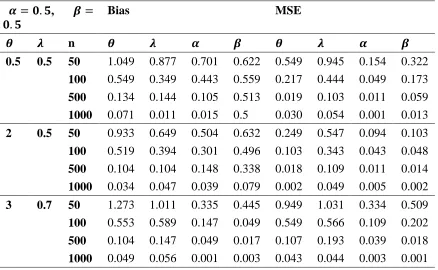
In this section, a brief simulation study is conducted to examine the performance of the MLEs of TGW parameters. Inverse transform method is used to generate random observations from TGW distribution. We generate 1000 samples of size, n =50, 100, 500 and n=1000 of TGW distribution. The evaluation of estimates was based on the bias of the MLEs of the model parameters, the mean squared error (MSE) of the MLEs. The empirical study was conducted with software R and the results are given in Table 1. The values in Table 1 indicate that the estimates are quite stable and, more importantly, are close to nominal values when 𝑛 goes to infinity. It is observed from Table 1 that the biases and MSEs decreases as n increases. The simulation study shows that the maximum likelihood method is appropriate for estimating the parameters of TGW distribution. In fact, the MSEs of the parameters tend to be closer to the zero when n increases. This fact supports that the asymptotic normal distribution provides an adequate approximation to the finite sample distribution of the MLEs. The normal approximation can be improved by using bias adjustments to these estimators.

Table 1: Biases and MSEs for the MLEs of the parameters of the TGW distribution 𝜶 = 𝟎. 𝟓, 𝜷 =

𝟎. 𝟓

Bias MSE

𝜽 𝝀 n 𝜽 𝝀 𝜶 𝜷 𝜽 𝝀 𝜶 𝜷

6. The log-transmuted geometric-Weibull (LTW-W) regression model

The TGW distribution with four parameters 𝛼 > 0, 𝜃 > 0, 𝑎 > 0 and 𝑏 > 0, introduced in Section 1. Let 𝑋 is a random variable following the TGW density function and 𝑌 is defined by 𝑌 = 𝑙𝑜𝑔(𝑋). The density function of 𝑌 obtained by replacing 𝛽 = 1/𝜎 and 𝜇 = −log(𝛼) reduces to

𝑓(𝑦) = 𝜃 𝜎exp[(

𝑦−𝜇 𝜎 )−exp(

𝑦−𝜇 𝜎 )]

[1+(𝜃−1){1−exp[−exp(𝑦−𝜇_𝜎 )]}]2[1 + 𝜆 −

2𝜆{1−exp[−exp(𝑦−𝜇

𝜎 )]}

1+(𝜃−1){1−exp[−exp(𝑦−𝜇_𝜎 )]}] (17)

where 𝑦 ∈ ℜ, 𝜇 ∈ ℜ, 𝜎 > 0, 𝜃 > 0 and 𝜆 > 0. We refer to Equation (17) as the LTGW distribution, say 𝑌: 𝐿𝑇𝐺𝑊(𝜃, 𝜆, 𝜎, 𝜇), where 𝜇 ∈ ℜ is the location parameter, 𝜎 > 0 is the scale parameter and 𝜃 and 𝜆 are shape parameters.

The corresponding survival function is

𝑠(𝑦) = 1 − 𝜃{1−exp[−exp( 𝑦−𝜇

𝜎 )]}

1+(𝜃−1){1−exp[−exp(𝑦−𝜇_𝜎 )]}[1 +

𝜆exp[−exp(𝑦−𝜇_𝜎 )]

1+(𝜃−1){1−exp[−exp(𝑦−𝜇_𝜎 )]}] (18)

and the hrf is simply ℎ(𝑦) = 𝑓(𝑦)/𝑆(𝑦). The standardized random variable 𝑍 = (𝑌 − 𝜇)/𝜎 has density function

𝑓(𝑧) = 𝜃exp[𝑧−exp(𝑧)]

[1+(𝜃−1){1−exp[−exp(𝑧)]}]2[1 + 𝜆 −

2𝜆{1−exp[−exp(𝑧)]}

1+(𝜃−1){1−exp[−exp(𝑧)]}] (19)

Parametric regression models to estimate univariate survival functions for censored data are widely used. A parametric model that provides a good fit to lifetime data tends to yield more precise estimates of the quantities of interest. Based on the LTGW density, we propose a linear location-scale regression model linking the response variable 𝑦_𝑖 and the explanatory variable vector 𝐯_𝑖𝑇 = (𝑣_𝑖1, . . . , 𝑣_𝑖𝑝) given by

𝑦_𝑖 = 𝐯_𝑖𝑇𝛃 + 𝜎𝑧_𝑖, i = 1, . . . , n (20)

where the random error 𝑧_𝑖 has density function (19), 𝛃 = (𝛽₁, … , 𝛽_𝑝)𝑇,𝜎 > 0, 𝜃 > 0 and 𝜆 > 0 are unknown parameters. The parameter 𝜇𝑖 = 𝐯𝑖𝑇𝛃 is the location of 𝑦𝑖. The

location parameter vector 𝜇 = (𝜇₁, … , 𝜇_𝑛)𝑇 _{is represented by a linear model 𝜇 = 𝑉𝛽,}

where 𝑉 = (𝑣1, … , 𝑣𝑛)𝑇 is a known model matrix.

Consider a sample (𝑦₁, 𝑣₁), … , (𝑦_𝑛, 𝑣_𝑛) of 𝑛 independent observations, where each random response is defined by 𝑦_𝑖 = min{log(𝑥_𝑖), log(𝑐_𝑖)}. We assume non-informative censoring such that the observed lifetimes and censoring times are independent. Let 𝐹 and 𝐶 be the sets of individuals for which 𝑦𝑖 is the log-lifetime or log-censoring,

respectively. The log-likelihood function for the vector of parameters 𝜏 = (𝛼, 𝜆, 𝜎, 𝛽𝑇)𝑇 from model (20) has the form 𝑙(𝜏) = ∑_𝑖∈𝐹 𝑙_𝑖(𝜏) + ∑_𝑖∈𝐶 𝑙_𝑖(𝑐)(𝜏), where 𝑙_𝑖(𝜏) = log[𝑓(𝑦_𝑖)], 𝑙_𝑖(𝑐)(𝜏) = log[𝑆(𝑦_𝑖)], 𝑓(𝑦_𝑖) is the density (17) and 𝑆(𝑦_𝑖) is the survival function (18) of 𝑌_𝑖. Then, the total log-likelihood function for 𝜏 reduces to

ℓ(𝜏) = 𝑟log (𝜃

𝜎) + ∑𝑖∈𝐹 (𝑧𝑖 − 𝑢𝑖) − ∑∈𝐹 log[1 + (𝜃 − 1){1 − exp[−𝑢𝑖]}] −2

+ ∑∈𝐹log[1 + 𝜆 −

2𝜆{1−exp[−𝑢𝑖]}

1+(𝜃−1){1−exp[−𝑢𝑖]}] + ∑_𝑖∈𝐶 log {1 − 𝜃{1−exp[−𝑢𝑖]}

[1 + 𝜆exp[−𝑢𝑖]

]}

where 𝑢_𝑖 = exp(𝑧_𝑖), 𝑧_𝑖 = (𝑦_𝑖 − 𝑣_𝑖𝑇𝛽)/𝜎 and 𝑟 is the number of uncensored observations (failures) and 𝑐 is the number of the censored observations. The MLE 𝜏̂ of the vector of unknown parameters can be evaluated by maximizing the log-likelihood (21). We use the statistical software R to determine the estimate 𝜏̂.

Under standard regularity conditions, the asymptotic distribution of (𝜏̂ − 𝜏) is multivariate normal 𝑁_𝑝+3(0, 𝐾(𝜏)−1_{), where 𝐾(𝜏) is the expected information matrix.}

The asymptotic covariance matrix 𝐾(𝜏)−1 of 𝜏̂ can be approximated by the inverse of the (𝑝 + 3) × (𝑝 + 3) observed information matrix −(𝜏). The elements of the observed

information matrix −Ł̈(𝜏), namely −Ł𝜃𝜃, −Ł𝜃𝜆,

−Ł_𝜃𝜎, −Ł_𝜃𝛽𝑗, −Ł_𝜆𝜆, −Ł_𝜆𝜎, −Ł_𝜆𝛽𝑗, −Ł_𝜎𝜎, −Ł_𝜎𝛽𝑗 and −Ł_{𝛽𝑗𝛽𝑠} for 𝑗, 𝑠 = 1, … , 𝑝, are evaluated numerically. The approximate multivariate normal distribution 𝑁_𝑝+3(0, −Ł̈(𝜏)−1) for 𝜏̂ can be used in the classical way to construct approximate confidence regions for some parameters in 𝜏.

7. Applications

In this section, we provide an application to real data set to illustrate the flexibility of the TGW distribution. The parameters are estimated by maximum likelihood method and R statistical software is used for computations. First, we describe the data sets and then determine the MLEs (and the corresponding standard errors) of the parameters. In order to compare models with the proposed distribution, we apply goodness-of-fit tests to verify which distribution fits better the real data set. The statistics Cramer von Mises (W*) and Anderson Darling (A*) are described in details in Chen and Balakrishnan (1995). The log-likelihood values and Akaike Information Criterion (AIC) are also obtained for all models and used to decide best model. In general, the smaller the values of these statistics, the better the fit to the data.

We compare the performance of the TGW distribution with other well-known families given in Table 2.

Table 2: Fitted families and their abbreviations

Families References

Weibull

Odd Log-Logistic-Weibull (OLL-W) da Cruz et al. (2014)

Kumaraswamy-Weibull (Kum-W) Cordeiro and de Castro (2011)

Exponentiated Generalized-Weibull (EG-W) Cordeiro et al. (2013)

Weibull-Weibull (W-W) Bourguignon et al. (2014)

Beta-Weibull (B-W) Eugene et al. (2002)

7.1. Strength of glass fibres

The data set represents the strength of 1.5 cm glass fibres, measured at National physical laboratory, England (see, Smith and Naylor [46]). The data are: 0.55, 0.93, 1.25, 1.36, 1.49, 1.52, 1.58, 1.61, 1.64, 1.68, 1.73, 1.81, 2.00, 0.74, 1.04, 1.27, 1.39, 1.49, 1.53, 1.59, 1.61, 1.66, 1.68, 1.76, 1.82, 2.01, 0.77, 1.11, 1.28, 1.42, 1.50, 1.54, 1.60, 1.62, 1.66, 1.69, 1.76, 1.84, 2.24, 0.81, 1.13, 1.29, 1.48, 1.50, 1.55, 1.61, 1.62, 1.66, 1.70, 1.77, 1.84, 0.84, 1.24, 1.30, 1.48, 1.51, 1.55, 1.61, 1.63, 1.67, 1.70, 1.78, 1.89.

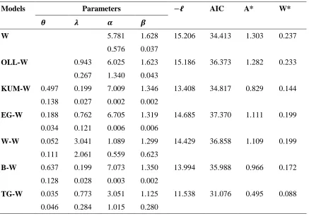
Table 3 gives W* and A* statistics, AIC and log-likelihood values. Based on Tables 2, it is clear that TGW distribution provides the overall best fit and therefore could be chosen as the more adequate model from other models for explaining the used data set.

Table3: Parameter estimations of fitted distributions

Models Parameters −𝓵 AIC A* W*

𝜽 𝝀 𝜶 𝜷

W 5.781 1.628 15.206 34.413 1.303 0.237

0.576 0.037

OLL-W 0.943 6.025 1.623 15.186 36.373 1.282 0.233

0.267 1.340 0.043

KUM-W 0.497 0.199 7.009 1.346 13.408 34.817 0.829 0.144

0.138 0.027 0.002 0.002

EG-W 0.188 0.762 6.705 1.319 14.685 37.370 1.111 0.199

0.034 0.121 0.006 0.006

W-W 0.052 3.041 1.089 1.299 14.429 36.858 1.109 0.199

0.111 2.061 0.559 0.623

B-W 0.637 0.199 7.073 1.350 13.994 35.988 0.966 0.172

0.128 0.028 0.003 0.002

TG-W 0.035 0.773 3.051 1.125 11.538 31.076 0.495 0.088

0.046 0.284 1.015 0.280

Figure 3: Fitted pdfs on histogram of first data set

7.2. Multiply censored relay data

The used data set represents the production relay and on a proposed design change (𝑛 = 35). Engineering experience suggested that lifetime has a Weibull distribution. Engineering sought to compare the production and proposed designs over the range of test currents. These data are also reported and analyzed in Cordeiro et al. (2017). LTGW regression model is adopted to analyze these data set. The variables involved in the study are: 𝑦_𝑖 - observed thounsands of cycles; 𝑐𝑒𝑛𝑠_𝑖 - censoring indicator (0=censoring, 1=lifetime observed) and 𝑥_𝑖1 - production (16 amps, 26 amps, 28 amps). We consider the following regression model

𝑦_𝑖 = 𝛽₁+ 𝛽₂𝑣_𝑖 + 𝜎𝑧_𝑖,

where 𝑦_𝑖 has the LTGW density (17), for 𝑖 = 1, … ,35. Table 4 lists the MLEs of the model parameters of the LTGW regression model fitted to the current data and the log-likelihood, AIC and BIC statistics. Based on the Table 4, it is clear that 𝛽₁ is statistically significant at the 5% level and then there is a significant difference among the levels of the production for the thousands of cycles.

Table 4: MLEs of the parameters (standard errors in parentheses and 𝒑-values in

[ ⋅ ]) and the log-likelihood, AIC and BIC measures.

Model 𝜽 𝝀 𝝈 𝜷𝟎 𝜷𝟏 −𝓵 AIC BIC LTGW 4.834 0.001 0.3257 7.504 -0.065 22.146 54.293 62.071

(0.625) (0.522) (3.104) (0.757) (0.014)

[< 0.001] [< 0.001]

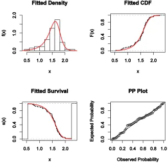
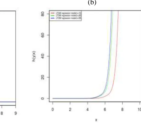
The plots in Figure 5(a) provide the Kaplan-Meier (KM) estimate and the estimated survival functions of the LTGW regression model. In view of Figure 5(a), there is no significant differences between the 26 and 28 amps levels survival functions. The plots of the hrf in Figure 5(b) corresponding to the thousands of cycles variable under the LTGW regression model indicate that the hrf is larger for 16 amps level than for 26 and 28 amps levels. Based on these plots, we conclude that the LTGW regression model provides a good fit to this data.

Figure 5: (a) Estimated survival functions and the empirical survival: LTGW regression model versus KM. (b) Fitted hrf using the LTGW regression model for the level production (16, 26 and 28 amps.).

8. Conclusions

We introduce the new lifetime distribution named the Transmuted Geometric-Weibull (TGW) distribution. Some of its mathematical properties are obtained. The maximum likelihood method is used to estimate the model parameters and the performance of the maximum likelihood estimators are discussed in terms of biases and mean squared errors. Two applications of the proposed family prove empirically its flexibility to model the real data sets. The log location-scale regression model based on a new generated distribution is introduced and discussed by means of real data application. Finally, it is clear that the proposed distribution provides better fits than other competitive models for used data sets.

References

1. Afify A. Z., Alizadeh, M., Yousof, H. M., Aryal, G. and Ahmad, M. (2016a). The transmuted geometric-G family of distributions: theory and applications. Pak. J. Statist., 32(2),139-160.

2. Afify, A. Z., Cordeiro, G. M., Yousof, H. M., Saboor, A., & Ortega, E. M. M. (2016). The Marshall-Olkin additive Weibull distribution with variable shapes for the hazard rate. Hacettepe Journal of Mathematics and Statistics, Forthcoming. 3. Alzaatreh, A., Lee, C., & Famoye, F. A. (2013). A new method for generating

families of continuous distributions, Metron 71, 63-79.

4. Aryal, G. R., & Tsokos, C. P. (2011). Transmuted Weibull distribution: a generalization of the Weibull probability distribution. European Journal of Pure and Applied Mathematics, 4, 89-102.

5. Aryal, G. R., & Elbatal, I. (2015). On the Exponentiated Generalized Modified Weibull Distribution. Communications for Statistical Applications and Methods, 22, 333-348.

6. Aryal, G. R., Ortega, E. M., Hamedani, G. G. & Yousof, H. M. The Topp-Leone Generated Weibull distribution: regression model, characterizations and applications, International Journal of Statistics and Probability, Forthcoming. 7. Balakrishanan, N., Leiva, V., Sanhuzea, A., & Cabrera, E. (2009). Mixture

inverse Gaussian distributions and its transformations, moments and applications. Statistics, 43, 91-104.

8. Chhikara, R. S., & Folks, J. L. (1989). The inverse Gaussian distribution, Marcel Dekker, New York.

10. Cordeiro, G. M., Hashimoto, E. M., & Ortega, E. M. M. (2014). The McDonald Weibull model. Statistics: A Journal of Theoretical and Applied Statistics, 48, 256-278.

11. Cordeiro, G. M., Ortega, E. M., & da Cunha, D. C. C. (2013). The exponentiated generalized class of distributions.

12. Cordeiro, G. M., Ortega, E. M., & Nadarajah, S. (2010). The Kumaraswamy Weibull distribution with application to failure data. Journal of the Franklin Institute, 347, 1399-1429.

13. Cordeiro, G. M., Ortega, E. M., & Silva, G. O. (2012). The Kumaraswamy modified Weibull distribution: theory and applications. Journal of Statistical Computation and Simulation, 84,1387-1411.

14. da Silva, R., Thiago, A., Maciel, D., Campos, R., & Cordeiro, G. (2013). A new lifetime model: the gamma extended Frechet distribution. Journal of Statistical Theory and Applications, 12, 39-54.

15. Efron, B. (1988). Logistic regression, survival analysis and the Kaplan-Meier curve. Journal of the American Statistical Association, 83, 414-425.

16. Elbatal, I., & Aryal, G. (2013). On the transmuted additive Weibull distribution. Austrian Journal of Statistics, 42, 117--132.

17. Famoye, F., Lee, C., & Olumolade, O. (2005). The Beta-Weibull Distribution, Journal of Statistical Theory and Applications, 4, 121-136.

18. Ghitany, M. E., Al-Hussaini, E. K., & Al-Jarallah, R. A. (2005). Marshall-Olkin extended Weibull distribution and its application to censored data. Journal of Applied Statistics, 32, 1025-1034.

19. Hanook, S., Shahbaz, M. Q., Mohsin, M., & Kibria, G. (2013). A Note on Beta Inverse Weibull Distribution, Communications in Statistics - Theory and Methods, 42, 320-335.

20. Khan, M. S., & King, R. (2013). Transmuted modified Weibull distribution: a generalization of the modified Weibull probability distribution. European Journal of Pure and Applied Mathematics, 6, 66-88.

21. Lai, C. D., Xie, M., & Murthy, D. N. P. (2001). Bathtub-shaped failure rate life distributions, Chapter 3, in Advances in Reliability, vol. 20 of Handbook of Statistics, pp. 69104.

22. Lai, C. D., Xie, M., & Murthy, D. N. P. (2003). A modified Weibull distribution. IEEE Transactions on Reliability, 52, 33-37.

23. Lee, C., Famoye, F., & Olumolade, O. (2007). Beta-Weibull distribution: some properties and applications to censored data. Journal of modern applied statistical methods, 6, 17.

24. Merovci, F. and Elbatal, I. (2013). The McDonald modified Weibull distribution: properties and applications. arXiv preprint arXiv:1309.2961.

26. Mudholkar, G. S., Srivastava, D. K., & Freimer, M. (1995). The exponentiated Weibull family: a reanalysis of the busmotor-failure data. Technometrics, 37, 436-445.

27. Mudholkar, G. S., Srivastava, D. K., & Kollia, G. D. (1996). A generalization of the Weibull distribution with application to the analysis of survival data. Journal of the American Statistical Association, 91, 1575-1583.

28. Nofal, Z. M., Afify, A. Z., Yousof, H. M., & Cordeiro, G. M. (2017). The generalized transmuted-G family of distributions. Communications in Statistics-Theory and Methods, 46:8,4119-4136.

29. Nofal, Z. M., Afify, A. Z., Yousof, H. M., & Louzada, F.(2016). Transmuted exponentiated additive Weibull distribution: properties and applications, Forthcoming.

30. Nofal, Z. M., Afify, A. Z., Yousof, H. M., Granzotto, D. C. T., & Louzada, F. (2016). Kumaraswamy transmuted exponentiated additive Weibull distribution. International Journal of Statistics and Probability, 5, 78-99.

31. Ortega, E. M. M., Cordeiro, G. M., & Hashimoto, E. M. (2011). A log-linear regression model for the Beta-Weibull distribution. Communications in Statistics- Simulation and Computations, 40, 1206-1235.

32. Pinho, L. G., Cordeiro, G. M., & Nobre, J. S. (2015). The Harris extended exponential distribution. Communications in Statistics- Theory and methods, 44, 3486-3502.

33. Provost, S. B., Saboor, A., & Ahmad, M. (2011). The gamma-Weibull distribution, Pak. Journal Stat., 27, 111--131.

34. Rezaei, S., Sadr, B. B., Alizadeh, M., & Nadarajah, S. (2016). Topp-Leone generated family of distributions: Properties and applications. Communications in Statistics- Theory and Methods, Forthcoming.

35. Sarhan, A. M., & Zaindin, M. (2009). Modified Weibull distribution, Applied Sciences,11, 123-136.

36. Shahbaz, M. G., Shahbaz, S., & Butt, N. M. (2102). The Kumaraswamy-inverse Weibull distribution. Pak. Journal Stat. Oper. Res., 8, 479-489.

37. Silva, G. O., Ortega, E. M. M., & Cordeiro, G. M. (2010). The beta modified Weibull distribution. Lifetime Data Analysis, 16, 409-430.

38. Xie, M., Tang, Y., & Goh, T. N. (2002). A modified Weibull extension with bathtub failure rate function. Reliability Engineering and System Safety, 76, 279-285.

39. Xie, M. & Lai, C. D. (1995). Reliability analysis using an additive Weibull model with bathtub-shaped failure rate function. Reliability Engineering and System Safety, 52, 87-93.