www.the-cryosphere.net/8/257/2014/ doi:10.5194/tc-8-257-2014
© Author(s) 2014. CC Attribution 3.0 License.
The Cryosphere
Solving Richards Equation for snow improves snowpack meltwater
runoff estimations in detailed multi-layer snowpack model
N. Wever1, C. Fierz1, C. Mitterer1, H. Hirashima2, and M. Lehning1,3
1WSL Institute for Snow and Avalanche Research SLF, Flüelastrasse 11, 7260 Davos Dorf, Switzerland 2Snow and Ice Research Center, NIED, Japan
3CRYOS, School of Architecture, Civil and Environmental Engineering, EPFL, Lausanne, Switzerland
Correspondence to: N. Wever ([email protected])
Received: 25 April 2013 – Published in The Cryosphere Discuss.: 5 June 2013
Revised: 16 December 2013 – Accepted: 19 December 2013 – Published: 20 February 2014
Abstract. The runoff from a snow cover during spring snowmelt or rain-on-snow events is an important factor in the hydrological cycle. In this study, three water balance schemes for the 1 dimensional physically-based snowpack model SNOWPACK are compared to lysimeter measure-ments at two alpine sites with a seasonal snow cover, but with different climatological conditions: Weissfluhjoch (WFJ) and Col de Porte (CDP). The studied period consists of 14 and 17 yr, respectively. The schemes include a simple bucket-type approach, an approximation of Richards Equation (RE), and the full RE. The results show that daily sums of snow-pack runoff are strongly related to a positive energy balance of the snow cover and therefore, all water balance schemes show very similar performance in terms of Nash-Sutcliffe ef-ficiency (NSE) coefficients (around 0.63 and 0.72 for WFJ and CDP, respectively) andr2values (around 0.83 and 0.72 for WFJ and CDP, respectively). An analysis of the runoff dynamics over the season showed that the bucket-type and approximated RE scheme release meltwater slower than in the measurements, whereas RE provides a better agreement. Overall, solving RE for the snow cover yields the best agree-ment between modelled and measured snowpack runoff, but differences between the schemes are small. On sub-daily time scales, the water balance schemes behave very differ-ently. In that case, solving RE provides the highest agreement between modelled and measured snowpack runoff in terms of NSE coefficient (around 0.48 at both sites). At WFJ, the other water balance schemes loose most predictive power, whereas at CDP, the bucket-type scheme has an NSE coeffi-cient of 0.39. The shallower and less stratified snowpack at CDP likely reduces the differences between the water
bal-ance schemes. Accordingly, it can be concluded that solving RE for the snow cover improves several aspects of modelling snow cover runoff, especially for deep, sub-freezing snow covers and in particular on the sub-daily time scales. The ad-ditional computational cost was found to be in the order of a factor of 1.5–2.
1 Introduction
An important coupling between the snow cover and sur-face or sub-sursur-face flow is provided by meltwater runoff at the base of the snowpack. For an accurate assessment of the snowpack runoff, it is important to have a good understand-ing of water movement through a snowpack. Water transport in snow is a complex process, because in general, the snow cover consists of many layers that may vary in temperature, density as well as in grain size and type. Experimental studies have shown that microstructural properties of the snowpack strongly influence the hydraulic properties of snow (Shimizu, 1970; Colbeck, 1974; Marsh, 1991; Yamaguchi et al., 2010). Where a snow layer with small grains is on top of a layer with coarse grains, these differences in hydraulic properties will lead to the formation of capillary barriers at the interface (Jordan, 1996; Waldner et al., 2004; Peitzsch et al., 2008; Mitterer et al., 2011). Also lateral flow along these capillary barriers, ice lenses or other dense parts of the snow cover has been identified (Peitzsch et al., 2008). Field experiments also have repeatedly observed the existence of preferential flow paths, which can provide a more efficient water trans-port mechanisms than matrix flow alone (e.g. Kattelmann, 1985; Schneebeli, 1995; Katsushima et al., 2013).
For modelling the water flow through the snowpack, cap-illary effects are often neglected and many models follow a bucket-type approach (e.g. Flerchinger and Saxton, 1989; Jin et al., 1999; Marks et al., 1999; Boone and Etchevers, 2001; Vionnet et al., 2012). These water balance schemes are easy to implement and computationally very efficient, mak-ing them very suitable for distributed modellmak-ing. Richards Equation (Richards, 1931), hereafter denoted as RE, is often applied to soils to describe variably saturated matrix flow. However, its application potential for snowpacks has already been identified in literature (Colbeck, 1972, 1974; Jordan, 1983; Illangasekare et al., 1990; Hirashima et al., 2010b). Jordan (1996) and Hirashima et al. (2010b) found that RE was able to reproduce the formation of capillary barriers as observed in laboratory experiments and snow profiles.
Compared to the knowledge of hydraulic properties in var-ious types of soil, measurements to derive hydraulic proper-ties in natural snow are restricted to a few studies (Shimizu, 1970; Colbeck, 1974; Marsh, 1991; Yamaguchi et al., 2010). Except for the study by Colbeck (1974), these studies were focussed on wet snow. Other snow types are more difficult to investigate, because in the presence of liquid water, snow metamorphism is rapid and the transition to wet snow types almost immediate.
Several snowpack models that describe liquid water trans-port on the basis of RE have been developed. Some model studies were restricted to idealised snowpacks to quantify the effects of water percolation in snow (Illangasekare et al., 1990; Jordan, 1996; Daanen and Nieber, 2009). When ne-glecting capillary forces, the resulting gravity flow in RE, as proposed by Colbeck (1972) in the kinematic wave model, has been used in earlier versions of CROCUS (Brun et al., 1989) and the current version of SNTHERM (Jordan, 1991;
Davis et al., 2001). Hirashima et al. (2010b) developed a wa-ter balance scheme where downward wawa-ter flow by Darcy’s law is approximated assuming stationary and equilibrium flow properties. To our knowledge, the full RE has not been used in a physically-based snow cover model to model water flow in snow in simulations of full snow seasons, forced by meteorological field measurements. In this study, the imple-mentation of a solver for RE in the physically-based snow-pack model SNOWPACK (Bartelt and Lehning, 2002; Lehn-ing et al., 2002a, b) is described, where the snowpack and soil are treated as a continuous column. The model is applied on two alpine measurement sites with a seasonal snow cover and contrasting climatological conditions: Weissfluhjoch (WFJ) near Davos, Switzerland and Col de Porte (CDP) near Greno-ble in France. In simulations of 14 and 17 snow seasons respectively, the bucket scheme, Hirashima et al. (2010b) scheme and the full RE are compared with lysimeter mea-surements of snowpack runoff. The focus will be primarily on the timing and magnitude of snowpack runoff.
2 Theory and numerical formulations
Several methods to model water flow in snow have been de-veloped. The three that are compared here, will be discussed below.
2.1 Bucket scheme
In the so-called bucket scheme, a threshold water content (water holding capacity,θh) is defined, above which all the liquid water exceeding this threshold in a layer is transported downward in the snowpack or soil, regardless of the storage capacity of lower layers (Bartelt and Lehning, 2002). The downward moving water is either stored at one of the lower layers (if possible), or is drained from the model domain. In SNOWPACK, the water holding capacity varies per layer ac-cording to (Coléou and Lesaffre, 1998):
θh=
0.0264+0.0099(1−θiθi), θi≤0.23
0.08−0.1023(θi−0.03) , 0.23< θi≤0.812
0, θi>0.812
(1)
whereθiis the volumetric ice content of the snow (m3m−3). 2.2 Richards equation
RE describes water movement in variably saturated porous media (Richards, 1931). For a 1-dimensional column, RE can be written in a mixed-form, which can be discretized in a fi-nite difference approximation that ensures perfect mass bal-ance (Celia et al., 1990):
∂θ
∂t −
∂ ∂z
K(θ )
∂h
∂z+cosγ
where θ is the volumetric liquid water content (LWC, m3m−3),K is the hydraulic conductivity (m s−1),h is the pressure head (m),zis the vertical coordinate (m, positive upwards and perpendicular to the slope),γ is the slope angle andsis a source/sink term (m3m−3s−1).
For applying Eq. (2), a water retention curve has to be specified that relatesθtoh. For snow, it is common to take the van Genuchten (1980) model:
θ=θr+(θs−θr)
1+(α|h|)n−m
Sc , (3)
whereθris the residual water content (m3m−3),θsis the sat-urated water content (m3m−3) andαis a fit coefficient that is related to the maximum pore size in the medium.mandnare additional fit parameters that are related to the pore size dis-tribution. Sc is a correction factor proposed by Ippisch et al. (2006), who have shown the necessity of using an air entry pressure whenn≤2. Here, the correction is applied for all values ofn, with an air entry pressure of 0.0058 m, corre-sponding to a largest pore size of 5 mm.
Two parameterizations for the van Genuchten (1980) model have been published recently: Daanen and Nieber (2009) fitted the water retention curve based on several pub-lished experiments that were collected by Marsh (1991) and Yamaguchi et al. (2010) retrieved water retention curves from several snow samples in laboratory experiments. Daa-nen and Nieber (2009) determined the parametersαandn
for the van Genuchten model to be:
α=30(2rg)+12, (4)
and
n=0.800(2rg)+3, (5)
whererg is the mean grain radius (mm), corresponding to the classical grain size definition (Fierz et al., 2009). In this study we (primarily) refer to this classical grain size of a snow layer as the average size of its grains, where the size of a single grain or particle is its greatest extension measured in millimetres (Fierz et al., 2009; Baunach et al., 2001). This has to be distinguished from the optical equivalent grain size that is related to the specific surface area of snow (see, for example, Carmagnola et al., 2013; Fierz et al., 2009).
The parameterization forαproposed by Yamaguchi et al. (2010) is:
α=7.3(2rg)+1.9. (6)
For n, the original parameterization by Yamaguchi et al. (2010) was modified by Hirashima et al. (2010b) to be able to extend the parameterization beyond grain radii of 2 mm:
n=15.68e(−0.46(2rg))+1, (7)
where, for numerical stability, the upper grain radius limit is set to be 5 mm in this study.
In both parameterizations, the van Genuchten parameterm
is chosen as:
m=1−(1/n). (8)
Note that both parameterizations for the van Genuchten model for snow differ significantly. Therefore, both are taken into consideration in this study, where the Hirashima et al. (2010b) modifications of the Yamaguchi et al. (2010) param-eter set will be referred to as Yamaguchi and the Daanen and Nieber (2009) parameter set as Daanen.
To apply the van Genuchten model, alsoθsandθrneed to be defined. Forθs, it is common to take it equal to the pore space:
θs=(1−θi)
ρi
ρw
. (9)
Note that the correction factor at the right hand side en-sures that there is enough space when liquid water freezes and thereby expands. Forθr, Colbeck (1974) experimentally found a value of 0.07. Gravity drainage experiments by Ya-maguchi et al. (2010) showed values around 0.02, suggesting that additional suction could reduceθeven more. Cold fresh snow is initially completely dry and also phase changes can reduceθbelowθr, causing singularities in the van Genuchten model (Eq. 3).
To circumvent these problems, a pragmatic strategy was implemented for determiningθr: first, new snow layers were initialized with a very small value forθ ofθ/10, whereθ is the convergence criterion (see Appendix A). This means that new snow layers are initialized in a dry state from the perspective of the convergence criterion. Then, the residual water content for the current time step (θrt)is scaled between 0 and 0.02 according to:
θrt=minD0.02,maxDθrt−1, f·θw
EE
, (10)
wheref is a tuning factor, taken as 0.75 andθrt−1is the resid-ual water content from the previous time step.
For determining the hydraulic conductivity, the van Genuchten-Mualem model is used (Mualem, 1976; van Genuchten, 1980):
K(θ )=Ksat21/2
h
1−1−21/mmi
2
, (11)
whereKsat is the saturated hydraulic conductivity (m s−1) and2is the effective saturation:
2= θ−θr
θs−θr
. (12)
ForKsat, the proposed equation by Shimizu (1970) has been widely used for a long time:
Ksat=
ρ
wg
µ 0.077
rg
1000
2
exp(−0.0078θiρi)
whereρwandρiare the density of water (1000 kg m−3) and ice (917 kg m−3),g is the gravitational acceleration (taken as 9.8 m s−2) and µ is the dynamic viscosity (taken as 0.001792 kg (m s)−1).
Recently, Calonne et al. (2012) proposed a slightly differ-ent equation, based on calculations from tomography images:
Ksat=
ρ
wg
µ 0.75
res
1000
2
exp(−0.013θiρi)
, (14)
whereresis the equivalent sphere radius (m).
The largest difference between the parameterization of Shimizu (1970) and Calonne et al. (2012) is in the range of snow with low density and new snow or decomposing and fragmenting snow particles (Calonne et al., 2012). In the presence of liquid water, wet snow metamorphism is rapid and also densification occurs, which quickly reduces the differences between both parameterizations. We found that results marginally improve when using the equation from Calonne et al. (2012), so results presented here exclusively use Eq. (14). For this, we determine the optical grain radius from the simulated grain size following Vionnet et al. (2012) and use this as an approximation ofres.
In SNOWPACK simulations, the typical microstructural evolution of the snowpack results in an increase in snow grain radius when snow ages or experiences melt-freeze cy-cles. This will increase the saturated hydraulic conductivity. However, settling of the snow cover and subsequent melt cy-cles will increase the density, which will decrease the hy-draulic conductivity. In the simulations, the first effect is dominating, as grain size will generally increase by a fac-tor 3–8, thus influencingKsatby a factor 9 to 64 over a snow season. Snow density will increase by a factor 2–5, influenc-ingKsatby a factor 5 to 25 over a snow season for typical snow densities. Field experiments have shown that different temperature regimes may result in a different microstructural evolution of the snowpack and hence ofKsat(Domine et al., 2013).
2.3 NIED scheme
Hirashima et al. (2010b) developed a water balance scheme for the SNOWPACK model based on approximating the wa-ter transport by fluxes derived from Darcy’s law by assuming stationary flow properties for a time step and equilibrium in water flow between two layers. RE is not explicitly solved and only downward water movement is possible. Hirashima et al. (2010b) also used the earlier discussed modified water retention curve for the van Genuchten model by Yamaguchi et al. (2010). The study focussed primarily on the internal snowpack processes and achieved the reproduction of cap-illary barriers on the interface between layers with different grain sizes. In this study, we will refer to this water balance scheme as NIED.
3 Data and methods
3.1 Data Weissfluhjoch
The experimental site at the Weissfluhjoch (WFJ, 46.83◦N, 9.81◦E) is located at an altitude of 2540 m in the Swiss Alps near Davos. During the winter months, almost all precipita-tion falls as snow at this altitude. As a consequence, a con-tinuous seasonal snow cover builds up every winter, with a maximum snow height ranging from 153–366 cm over the period 1934–2012. The measurement site is located in an al-most flat part of a southeast oriented slope (γ is taken equal to 0).
The dataset contains air temperature, relative humidity, wind speed and direction, incoming and outgoing longwave and shortwave radiation, surface temperature, soil tempera-ture at a few cm below the surface, snow height and precip-itation from a heated rain gauge. The dataset has been qual-ity checked, by replacing missing values with values from backup sensors or by applying various interpolation methods (Schmucki et al., 2013). The precipitation was corrected for undercatch during snowfall and windy conditions by using a correction proposed by Førland et al. (1996). The relation-ship for a Finnish H&H-90 gauge was taken, as it was em-pirically found to estimate precipitation at WFJ best, when comparing seasonal maximum measured snow water equiv-alent (SWE) in biweekly manual snow profiles to modelled SWE at the same date.
The experimental site is equipped with a lysimeter, which measures the liquid water runoff from the snowpack. The surface area of the squared lysimeter is 5 m2 and since 2001, it is measuring at a resolution of 0.16 kg m−2 (be-fore 0.20 kg m−2). Data is collected at 10 min intervals. The lysimeter is enclosed by a 60 cm high wall to reduce lateral flow effects near the soil-snow interface. However, lateral flow along capillary barriers within the snow cover or other, more impermeable layers (e.g. melt-freeze crusts) higher in the snowpack may still affect the measurements. The lysime-ter is expected to collect additional meltwalysime-ter advected by lateral flow mechanisms, as the device is located close to the lowest part of the site.
The studied period for WFJ is from 1 September 1996 to 30 September 2010. This period, consisting of 14 full winter seasons, is chosen based on data-availability and quality of the lysimeter measurements.
3.2 Data Col de Porte
snowpack runoff more often during the snow season and ROS events are more frequent than at WFJ. Due to these frequent wetting cycles, we expect the snowpack to be less stratified at CDP than at WFJ. A snow cover builds up for at least several weeks every winter season at this site, but is in-terrupted by complete melt in some years. With typical max-imum snow heights ranging from 68–207 cm over the period 1993–2011, snow covers at CDP are generally less deep than at WFJ.
The dataset contains a set of very similar measurements as at WFJ: air temperature, specific humidity, wind speed and direction, incoming and outgoing longwave and short-wave radiation, surface temperature, several soil tempera-tures, snow height and precipitation from a heated rain gauge. The precipitation data in the CDP dataset is already corrected for undercatch and the precipitation amounts are separated in rain and snow, as described in Morin et al. (2012). The SNOWPACK model accepts only a single value as precip-itation input and decides based on a temperature threshold of 1.2◦C whether the precipitation should be considered rain or snow. Therefore, we adjusted the CDP dataset to an air temperature above 1.2◦C in case only rainfall was reported, and an air temperature below 1.2◦C in case snow fall was re-ported. Mixed precipitation was provided as a sum to SNOW-PACK and depending on the air temperature considered as rain or snowfall.
CDP is equipped with both a 5 m2and a 1 m2 lysimeter. Kattelmann (2000) shows that smaller lysimeters exhibit sig-nificantly larger inaccuracies. Also in this study we found that the larger lysimeter provided highest agreement for all water balance schemes, and we will only use the data from the 5 m2 lysimeter. The dataset from CDP is used here for the period from 1 September 1994 to 31 July 2011 (17 win-ter seasons), dewin-termined by the data availability of the 5 m2 lysimeter.
3.3 Methods
3.3.1 Model description
The 1-dimensional mixed form of RE (Eq. 2) is solved by a Picard iteration scheme (Celia et al., 1990), adapted for a variable grid spacing based on Rathfelder and Abriola (1994). The scheme has the property of an easy numerical implementation that is globally convergent. In Appendix A, several aspects of the numerical implementation are dis-cussed.
When using RE, the snowpack and the soil are considered as a single continuous column. There are no special boundary conditions for the lowest snow layer or upper-most soil layer. The snowpack runoff, defined as all liquid water leaving the snowpack at the bottom, is calculated in a model postprocess-ing step by evaluatpostprocess-ing Darcy’s law at the interface between
the snowpack and the soil:
q=K
∂h
∂z +cosγ
≈Ki+1/2
hi+1−hi
1z +cosγ
, (15)
whereq is the snowpack runoff (m s−1), positive values noting downward water movement. The right hand side de-scribes the numerical implementation, wherei denotes the upper-most soil element andi+1 the lowest snow element,
Ki+1/2is the hydraulic conductivity at the interface between elementiandi+1, andhi andhi+1are the pressure heads in the top soil and bottom snow element, respectively.1zis the vertical grid spacing. In the rest of the paper, snowpack runoff will be treated from a mass balance perspective, de-noting downward water movement (snowpack outflow) with a negative value.
For the snowpack, the layer thickness varies per layer and with time. When there is solid precipitation, new snow lay-ers are added on top of the domain with an initial thickness of 2 cm. Over time, settling of the snow reduces the layer thickness. When a snow layer gets smaller than a specified minimum height or the ice content decreases below a speci-fied minimum value, it is joined with the layer above (in case it is the lowest snow layer) or below (all other cases). When two adjacent snow layers get similar properties, they are also merged (Bartelt and Lehning, 2002).
may be formed on the snow cover (Stössel et al., 2010). In case of evaporation or sublimation, the implementation of the boundary condition require different treatments, depending on water balance scheme. In the bucket and NIED simulations, the latent heat flux is first used to evaporate liquid water from the snowpack. Remaining energy is then used to sublimate the ice matrix, respecting the fact that evaporation is more favoured by the lower energy required for evaporation. When RE is used for the snowpack, the specified flux at the upper boundary is actively limited. A maximum evaporative flux is allowed, based on an imaginary limiting pressure head outside the model domain (see Appendix A). If the evaporative flux exceeds this value, the flux is limited to this value. The excess energy is used to sublimate the ice matrix. Note that the actual mass exchange differs whether evaporation/condensation or sublimation/deposition occurs, because of the difference in latent heat involved. This may cause a slightly different mass balance of the snowpack in the different simulations. 3.4 Simulation setup
The SNOWPACK model is driven by the measured precipi-tation amounts. Measured precipiprecipi-tation is assumed to be rain when the air temperature was higher than 1.2◦C and snow otherwise. The net radiation is determined from the incoming and outgoing longwave and shortwave radiation and, conse-quently, albedo is derived from the measured shortwave ation components. Absorption of penetrating shortwave radi-ation is treated as a source term for the temperature equradi-ation in the top snow layers. The surface energy balance is eval-uated using the net longwave radiation and calculated latent and sensible heat fluxes using a common form of Monin– Obukhov bulk formulation (Lehning et al., 2002a). Atmo-spheric stability is estimated from the difference in measured air and surface temperature. The net heat flux is used as a Neumann boundary condition for the temperature equation. In the simulations, a roughness length (z0) of 0.002 m was used for WFJ (Stössel et al., 2010) and 0.015 m for CDP (Es-sery et al., 2013).
In all simulations, the water flow in the soil is solved using RE. Soil freezing was not considered and the soil temperature was bounded by 0◦C. This assumption is supported by snow profiles of seasonal snow covers, where ground heat creates close to melting conditions at the snow-soil interface.
For WFJ simulations, a soil of 1.5 m depth is used, divided into 30 layers of varying thickness. This setup ensures that choices for lower boundary conditions in the soil are only marginally impacting the snow cover. Typical soil proper-ties for gravel/coarse sand were taken (θr=0.01,θs=0.35,
α=3.5 m−1,n=4.5 andKsat=3.171·10−6m s−1). At the lower boundary, a water table is prescribed as a Dirichlet boundary condition for RE and a constant upward soil heat flux of 0.06 W m−2is prescribed as Neumann boundary con-dition for the temperature equation. Although in reality, the
water table is expected to be deeper at WFJ, the gravel/coarse sand material will make the influence of the water table on snowpack runoff negligible small.
At CDP, the ground heat flux is an important factor in the energy balance of the snowpack, due to the low elevation and consequently warmer soil of the site. To take this into account in the simulations, a soil of 10 cm depth was used, divided into 10 layers, and measured soil temperatures at 10 cm depth were applied as a Dirichlet boundary condition for the lower boundary. Although Morin et al. (2012) reports a substantial loam content for the soil at CDP, we used the same soil as for WFJ to prevent ponding conditions in the shallow soil. At the lower boundary, a free drainage Neumann boundary condition was applied for solving RE.
3.4.1 Analysis
For both sites, the model simulations and lysimeter measure-ments are analysed for the 24, 12, 6, 3 and 1 h time scales and, only for WFJ, also for the 0.5 h time scale. Runoff values were constructed by summing the 15 min model output reso-lution or the 10 min (WFJ)/1 h (CDP) lysimeter measurement resolution to the respective time scales, starting at 00:00 h (midnight) local time. We restrict the analysis in this study only to periods with a snow cover on the ground during the winter season. We will refer to these periods as snow seasons, where the snow seasons are denoted by the year in which they end (e.g. 1997 denotes winter season 1996–1997). Summer snowfalls are ignored in the analysis.
To determine the beginning and end of a snow season at WFJ, it is assumed that on 1 March a snow cover is al-ways present. Then, it is searched both forward and back-ward in time in the measurements and simulations until all have snow-free conditions. These mark the start and end of the snow season. The melt season at WFJ is defined here as the period from 1 March to the melt out date. In the measure-ments from the lysimeter, one cannot distinguish snowpack runoff with a snowpack present and rain without a snowpack. Using measured snow height to determine the end of the snow season appeared to be somewhat cumbersome as mea-surement inaccuracies make it difficult to determine when the surface is snow free. Moreover, the rain gauge used to derive precipitation amounts, the snow height sensor and the lysimeter are located several metres apart. Given the spatial variability of the snow cover thickness, the snow height sen-sor cannot be regarded as fully representative for the snow height at the lysimeter. Therefore, the snowpack runoff mea-sured by the lysimeter was assumed to come from the snow-pack as long as a snow cover was present in the simulations and consequently, the lysimeter runoff may include rainfall in snow-free conditions, if the duration of the simulated snow cover exceeds the real snow cover presence.
the snow cover present at 31 December. If at May 1, no snow cover is present, it is looked backward in time to find the last day where a snow cover is present in either the measurements or one of the simulations. Else, we look forward in time, to find the last day a snowcover is present. The lysimeter data from CDP is cleaned by the providers such that it only re-ports values when a snow cover is present. However, if the snow cover still exists in the simulations and the lysimeter is already snow-free, rainfall will be added to snowpack runoff in the simulations, but is not reported by the lysimeter. There-fore, rainfall was added to the lysimeter series when there was no measured snow cover, but still a snow cover in one of the simulations.
To assess the added value of the water balance schemes, the performance of modelled snowpack runoff is compared to a constructed runoff series that consists of the modelled LWC production (snowmelt, refreezing and rain input). This LWC production is calculated for each time step as the av-erage of the four simulation variants. It represents the case where the sum of snowmelt and rain input is routed to runoff immediately and it will be referred to as average LWC pro-duction (avg. LWC prod.).
To quantify the accuracy of the modelled snowpack runoff, Nash-Sutcliffe model efficiency coefficients (NSE, Nash and Sutcliffe, 1970) are calculated for all time scales. These are only determined over the winter snow season. To calculate an NSE coefficient over all snow seasons, the snow seasons are analyzed sequentially by removing the intermediate summer periods.
All simulations were run on the same desktop computer as a single-core process. The increase in computational time by using RE for the snow cover is significant but not excessive: the additional effort for water transport is of the same order as the total seasonal snow cover simulation without RE. For WFJ, the simulations with the bucket scheme for snow took on average about 1.5 min per year and the NIED scheme took about 1.7 min per year. Solving RE for snow increased the average simulation time to 3.1 min per year for RE (Yam-aguchi) and 2.7 min per year for RE (Daanen). CPU times for CDP are about half as those for WFJ, as a result of the shallower snowpack.
4 Results and discussion
The discussion of the results will first focus on the seasonal and daily time scale and afterwards on sub-daily time scales. Table 1 shows the snow season period and the maximum measured snow height for each year. In the studied period, the snow season at WFJ is mostly starting in October, and the melt out date is mostly between mid-June and mid-July. The maximum measured snow height ranges from 182 cm in 2005 to 356 cm in 1999. At CDP, the snow season is shorter than at WFJ and is roughly between November and April/May. Also the maximum snow height reached is lower
than at WFJ, and ranges from 68 cm in the years 2001 and 2007 to 207 cm in 1999.
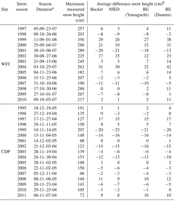
Table 1 also shows the seasonal average difference be-tween measured and modelled snow height. The year-to-year variability indicates that using measured precipitation to drive snowpack simulations has some inherent inaccuracies and the main problem is that the over- or underestimation of a single precipitation event will persist throughout the rest of the snow season. It is noteworthy that snow height also varies between the different schemes, although these variations are smaller than the year-to-year ones. The snow height varia-tions between simulavaria-tions can be explained by differences in mass loss due to runoff and by differences in settling, as a result of varying vertical LWC and density distributions due to the different water balance schemes. Although the differ-ences between simulations are rather small, RE with Yam-aguchi’s parameterization shows the smallest deviation from measured snow height, whereas Daanen’s parameterization seems to cause slower settling and higher snow heights. This is especially visible in the simulations for WFJ.
Figure 1 shows that the cumulative runoff sum from the snowpack exhibits much smaller variations between simulations than the snow height, indicating that there is only a small difference in modelled snow water equiva-lent. As the precipitation input is the same for all simula-tions, the slightly varying cumulative runoff sums are mainly caused by differences in evaporation/condensation or sub-limation/deposition. The reasons for these differences are, first, that the LWC in the surface layer will influence the sur-face temperature, especially due to variations in time needed to refreeze at night. These differences in surface temperature in the evening hours may influence sensible and latent heat exchange and may cause differences in energy input into the snow cover between simulations. Second, the partitioning of latent heat between sublimation and evaporation is different between the water balance schemes. Because of the differ-ence in latent heat associated with sublimation or evapora-tion, mass gain or loss will be smaller in case of sublima-tion/deposition than in evaporation/condensation. Note that in practise, the albedo of the snow cover, and thus the energy balance, is also influenced by the LWC in the surface layer. This influence is not present here, because measured albedo is used to drive simulations at both sites.
Table 1. Durationa, maximum measured snow height and seasonal average difference in measured and modelled snow heightbfor all snow seasons.
Snow Season Maximum Average difference snow height (cm)b
Site season Durationa measured Bucket NIED RE RE
snow height (Yamaguchi) (Daanen) (cm)
WFJ
1997 05-09–23-07 257 6 3 4 11
1998 09-10–26-06 203 −8 −9 −8 −2
1999 11-09–01-08 356 29 26 27 38
2000 25-09–04-07 288 21 19 15 31
2001 30-10–08-07 289 −20 −21 −18 −13
2002 30-08–27-06 225 17 15 12 23
2003 21-09–15-06 245 3 3 7 14
2004 03-10–25-07 262 31 30 32 42
2005 04-11–23-06 182 7 6 6 14
2006 15-11–25-06 207 −2 −3 −2 5
2007 31-10–10-06 190 −11 −11 −10 −5
2008 17-10–30-06 288 0 0 2 11
2009 27-10–01-07 267 −7 −8 −8 1
2010 09-10–03-07 217 2 1 5 11
CDP
1995 18-12–18-05 191 3 1 2 4
1996 27-12–19-04 135 0 −3 −2 0
1997 17-11–27-04 127 17 15 15 17
1998 29-11–11-05 158 8 5 5 7
1999 10-11–14-05 207 −20 −23 −21 −20
2000 15-11–04-05 148 −14 −16 −16 −14
2001 14-12–02-05 68 0 0 0 1
2002 21-12–03-04 123 −14 −15 −16 −15
2003 28-11–19-04 139 −4 −6 −6 −4
2004 26-11–30-04 153 −12 −13 −13 −10
2005 28-11–02-05 168 1 0 0 2
2006 22-11–02-05 158 −5 −6 −4 −3
2007 05-12–11-04 68 −2 −3 −4 −3
2008 08-11–08-05 140 11 9 10 12
2009 20-11–23-04 143 −6 −7 −6 −5
2010 29-11–25-04 105 −1 −2 −1 0
2011 06-11–07-04 72 9 8 10 10
aThe snow season duration is formatted in DD-MM and denotes the period for which a snow cover existed in either the measurements or one of the model variants.
bA positive value denotes an overestimation of snow height in the model compared to measured snow height (and vice versa).
The discrepancies between modelled and measured runoff may also be caused by an unrepresentative snowpack state at the lysimeter or inhomogeneous flow features like flow fingering and flow over ice lenses. The accuracy of the un-dercatch correction for solid precipitation (Goodison et al., 1998) may also vary from year-to-year. Furthermore, the de-viations are likely a general expression of the fact that snow height can vary over short distances, mainly caused by het-erogeneity in wind fields (e.g. Winstral et al., 2002; Mott et al., 2010). However, the deviation between measured and modelled snowpack runoff is suspiciously large at WFJ in the years 1997 and 2000. These differences seem to be too large to be explained by lateral flow effects or inhomoge-neous snow redistribution, and the agreement between
mea-sured and modelled snow height for these years (see Table 1) suggest that precipitation input is also not the cause of the differences. In both cases, the consistency between maxi-mum measured snow height and modelled snowpack runoff indicates that the most probable source of error is in the mea-sured snowpack runoff. This likely is either a malfunction-ing of the lysimeter or a strongly unrepresentative snowpack state at the lysimeter.
4.1 Daily time scale
−3500 −3000 −2500 −2000 −1500 −1000 −500 0
1998 2000 2002 2004 2006 2008 2010
Runoff sum (mm)
Year
Measured Bucket NIED RE (Yamaguchi) RE (Daanen) Avg. LWC prod. (a)
−1600 −1400 −1200 −1000 −800 −600 −400 −200 0
1996 1998 2000 2002 2004 2006 2008 2010
Runoff sum (mm)
Year
Measured Bucket NIED RE (Yamaguchi) RE (Daanen) Avg. LWC prod. (b)
Fig. 1. Measured and modelled snowpack runoff sums (mm) over
the snow seasons for WFJ (a) and CDP (b).
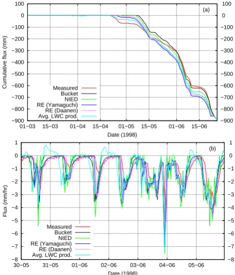
the modelled runoff sum. Therefore, this year is used as an example. Figure 2a shows the cumulative snowpack runoff in the melt season. As can be seen, the lysimeter registers the first melt water at the base of the snowpack earlier than any of the model schemes. The simulations with RE pro-duce runoff soon after the first measured runoff, whereas the bucket and NIED simulations show some delay. For the rest of the melt season, there are no important differences. Be-cause the bucket and NIED simulations withhold the water too much in the snowpack compared to the lysimeter and the simulations with RE, the daily outflow near the end of the season becomes higher than in simulations with RE. Gen-eral runoff dynamics and alternating phases with high and low runoff are represented well in all simulations, although in some periods, discrepancies in runoff amounts between measurements and model exist.
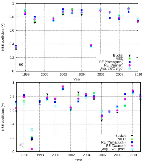
Figure 3 shows the NSE coefficients for daily sums of snowpack runoff for both WFJ and CDP for the respec-tively 14 and 17 yr individually. It shows that for the daily time scale, differences between the various models are much smaller than year-to-year differences in NSE coefficients. Furthermore, the spread between simulations is larger at CDP than WFJ. For both sites, it can be seen that when the agreement between modelled and measured snowpack runoff is lower, all water balance schemes have a lower agreement with measured snowpack runoff (and vice versa). The fact that NSE coefficients for the average LWC production
fol-−900 −800 −700 −600 −500 −400 −300 −200 −100 0 100
01−03 15−03 01−04 15−04 01−05 15−05 01−06 15−06 −900 −800 −700 −600 −500 −400 −300 −200 −100 0 100
Cumulative flux (mm)
Date (1998) Measured
Bucket NIED RE (Yamaguchi) RE (Daanen) Avg. LWC prod.
(a)
−8 −7 −6 −5 −4 −3 −2 −1 0 1
30−05 31−05 01−06 02−06 03−06 04−06 05−06 −8 −7 −6 −5 −4 −3 −2 −1 0 1
Flux (mm/hr)
Date (1998) Measured
Bucket NIED RE (Yamaguchi) RE (Daanen) Avg. LWC prod.
(b)
Fig. 2. Cumulative snowpack runoff at WFJ for the lysimeter
mea-surements and the various water balance schemes for the 1998 melt season (a) and hourly snowpack runoff for the lysimeter measure-ments and the various water balance schemes for one week during the 1998 melt season (b).
low the same pattern is an indication that for these years, sources of error causing variation of NSE coefficients may be related to the estimation of meltwater production as deter-mined by a positive energy balance and a possibly sometimes inaccurate partitioning of precipitation in rain and snow. The representation of internal snowpack structure and accompa-nying hydraulic properties in the model seem to play a less pronounced role, which may also imply that the model does not reproduce adequately enough year-to-year variations in internal snowpack structure that influence water flow.
0 0.2 0.4 0.6 0.8 1
1998 2000 2002 2004 2006 2008 2010
NSE coefficient (−)
Year
Bucket NIED RE (Yamaguchi) RE (Daanen) Avg. LWC prod. (a)
0 0.2 0.4 0.6 0.8 1
1996 1998 2000 2002 2004 2006 2008 2010
NSE coefficient (−)
Year
Bucket NIED RE (Yamaguchi) RE (Daanen) Avg. LWC prod. (b)
Fig. 3. NSE coefficients (model vs. measured) for the snow seasons
for the 24 h time scale for WFJ (a) and CDP (b). The NSE coeffi-cients for snow season 2000 for WFJ are negative and not shown.
the shadowing effect of the wall. This may lead to a non-representative snow cover inside the lysimeter.
The three years with a very low NSE coefficient for WFJ are also likely related to measurement problems. Typical causes for low NSE values are a consistent over- or under-estimation (bias) and poor timing of meltwater peaks (Mc-Cuen et al., 2006). For the years 1997 and 2000, the low NSE coefficients are for an important part caused by the bias between modelled and measured seasonal snowpack runoff (see Fig. 1). For the year 2005, it appears as if the lysimeter was obstructed for quite some time, after which half the sea-sonal sum of snowpack runoff passed through the device in few days time (not shown).
In terms of NSE coefficient, RE does reproduce measured snowpack runoff best at both sites, although differences are marginal. At WFJ, RE achieves an NSE coefficient of 0.63 and 0.62 for Yamaguchi’s and Daanen’s parameterization, respectively, over all 14 snow seasons. Bucket and NIED schemes also exhibit very similar performance with NSE co-efficients of 0.61 and 0.62, respectively. For CDP, NSE coef-ficients for the daily time scale are higher than for WFJ. RE achieves an NSE of 0.72 and 0.71 for Yamaguchi’s and Daa-nen’s parameterization, respectively. NSE coefficients for the bucket and NIED scheme are 0.70 and 0.72, respectively. The fact that the different water balance schemes have very sim-ilar performance on the daily time scale and have an NSE coefficient very similar to the one for the average LWC
pro-duction is an indication that once the snowpack is isothermal, meltwater production near the surface is transported down-ward within the day in all models and that this is in good agreement with the measurements. This is noted already in literature (e.g. Colbeck, 1972; Brun et al., 1989; Davis et al., 2001).
4.2 Timing of seasonal runoff
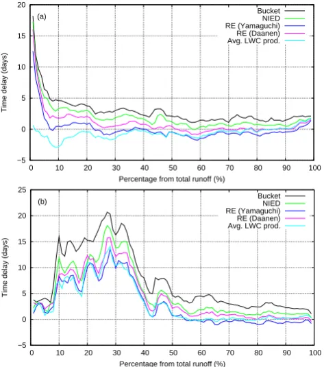
To assess the performance of the water balance schemes in simulating the dynamics of the snowpack runoff over the sea-son, it was determined at which date a certain percentage of the total cumulative snowpack runoff was reached. This was also done for the measurements. Then the difference be-tween measured and modelled date was determined. Figure 4 shows the time delay in days between modelled and mea-sured snowpack runoff. A positive delay means that modelled cumulative snowpack runoff arrives later in time than the measured one. For example: 20 % of total snowpack runoff is delayed by 1 day in the RE (Yamaguchi) simulations and 4 days in the bucket simulations. For CDP, the comparison is made over the complete snow season, as important melt and snowpack runoff events occur throughout the season. At WFJ, melt and subsequent snowpack runoff occurs either at the early start of the snow season (October or November), or after the beginning of March. So for WFJ, the comparison is made for the spring melt season only.
As can be seen, all models are strongly underestimating the arrival date of the first few percent of the total snowpack runoff in the melt season at WFJ, up to about 18 days for the bucket and NIED scheme. Average LWC production in the models is in fairly good agreement with measured snowpack runoff, suggesting that the first surface melt is almost directly accompanied by snowpack runoff. This fast arrival of melt-water at the base of the snowpack in the measurements likely results from the more efficient transport mechanism of pref-erential flow paths compared to matrix flow. Several experi-ments have shown that water flow in snow is not horizontally homogeneous (e.g. Conway and Benedict, 1994; Waldner et al., 2004; Katsushima et al., 2013). The 1-D approach in this study cannot resolve preferential flow paths by flow fin-gering, as observed in several experiments. Preferential flow paths will be able to transport water downward faster than horizontally uniform matrix flow, as simulated here. How-ever, Fig. 4 suggest that this may involve only about 5 % of cumulative seasonal snowpack runoff. Note that this does certainly not imply that preferential flow cannot have a more pronounced effect on the internal snowpack microstructure or wet snow avalanche formation.
−5 0 5 10 15 20
0 10 20 30 40 50 60 70 80 90 100
Time delay (days)
Percentage from total runoff (%)
Bucket NIED RE (Yamaguchi) RE (Daanen) Avg. LWC prod. (a)
−5 0 5 10 15 20 25
0 10 20 30 40 50 60 70 80 90 100
Time delay (days)
Percentage from total runoff (%)
Bucket NIED RE (Yamaguchi) RE (Daanen) Avg. LWC prod. (b)
Fig. 4. Average delay over all simulated years between modelled
and observed snowpack runoff as a function of percentage of total melt season snowpack runoff (for WFJ (a), starting 1 March) or total snow season snowpack runoff (for CDP, b).
leaving the snowpack is in quite good agreement with mea-sured values. The delayed snowpack runoff in the bucket and NIED scheme persist for almost the entire season. Appar-ently, bucket and NIED are retaining meltwater in the snow-pack too long, releasing it later in the melt season.
At CDP, the first modelled snowpack runoff in the snow season is in rather good agreement with the measurements. This is likely a result of the fact that the snowpack is still very shallow when these snowpack runoff events occur. Af-terwards, there arises a marked delay, visible in all water bal-ance schemes, but most pronounced in the bucket scheme. In this period, extending from about 8–40 % of the snowpack runoff, more snowpack runoff is measured than modelled. This may be an expression of efficient preferential flow paths. After about 40 %, all water schemes are fairly constant com-pared to the beginning of the snow season. It may be con-cluded that the variations in the RE and NIED schemes are smaller than in the bucket scheme, showing that they provide better representation of the runoff dynamics throughout the snow season.
4.3 Sub-daily time scales
Figure 2b shows the hourly flux of snowpack runoff for one week during the melt season of the example snow season 1998. A daily returning peak in melt water outflow,
associ-ated with the daily cycle in melt, is visible. During 3 June a ROS event occurred with 14 mm of rain. The daily onset of runoff and timing of the peak flux is better reproduced by simulations with RE. The figure also shows that RE is able to reproduce the recession curve in the evening hours and the night. Although the NIED scheme does not reproduce this for WFJ in this case, Hirashima et al. (2010a) found that the recession curve is reproduced in the NIED scheme for warm snow regions such as the central part of Japan.
In Fig. 5, NSE coefficients for the various water balance schemes are shown for sub-daily time scales. It is clear that for smaller time scales, the NSE coefficients decrease for all water balance schemes. On the 12 and 24 h time scales, all schemes produce more or less similar results at both sites. For the 1 h time scale, RE (Yamaguchi) achieves a still rea-sonable NSE coefficient of 0.49 for WFJ, where the bucket and NIED scheme have NSE coefficients of 0.17 and 0.07, respectively. The decrease in NSE coefficient for the bucket and NIED schemes must be mainly caused by poor timing of the meltwater release, as the daily sums of modelled snow-pack runoff do not show large differences (see Fig. 3). At CDP, the RE scheme achieves a similar NSE coefficient for the 1 h time scale as at WFJ (respectively 0.47 and 0.44 for the Yamaguchi and Daanen parameterization). On the other hand, the bucket scheme achieves a much better NSE coef-ficient than at WFJ (0.39). Although an exact reason for the contrasting results was not found, we think it is a confirma-tion of the fact that once the snowpack is isothermal, dif-ferences in water balance schemes are rather small. These snowpack conditions are more frequent at CDP than at WFJ. Moreover, the shallower and less stratified snowpack at CDP likely reduces the differences between the water transport as calculated by the different schemes.
The constructed runoff series from the average LWC pro-duction shows a strong decrease in NSE coefficient on the smaller time scales, indicating the importance of taking into account travel time and intermediate storage in the snow cover for sub-daily time scales.
−0.3 −0.2 −0.1 0 0.1 0.2 0.3 0.4 0.5 0.6 0.7
24 12 6 3 1 0.5
Nash−Sutcliffe Model Efficiency (−)
Time scale (hours) Bucket
NIED RE (Yamaguchi) RE (Daanen) Avg. LWC prod.
(a)
0 0.1 0.2 0.3 0.4 0.5 0.6 0.7 0.8
24 12 6 3 1
Nash−Sutcliffe Model Efficiency (−)
Time scale (hours) Bucket
NIED RE (Yamaguchi) RE (Daanen) Avg. LWC prod.
(b)
Fig. 5. NSE coefficients (model vs. measured) over all snow seasons
for the studied water balance schemes for different sub-daily time scales for WFJ (a) and CDP (b).
4.4 Timing of hourly runoff
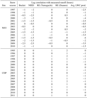
The NSE coefficients for WFJ simulations on the hourly time scale were close to 0 or even negative for the bucket and NIED schemes, which was ascribed to poor timing of the meltwater release in the bucket and NIED simulations. To quantify the timing of snowpack runoff, lag correlations were calculated between each of the simulations and the measured snowpack runoff. The time span was limited to −12 and
+12 h, to prevent correlations with the daily cycle. Table 2 shows the time lag belonging to the highest lag correlation, with negative values indicating the snowpack runoff is too early in the day in the simulations. For WFJ, the bucket and NIED schemes have about 1–2 h too early snowpack runoff compared to measured snowpack runoff, while both simula-tions with RE show fairly good agreement in timing. Yam-aguchi’s parameterization seems to provide the best agree-ment with the measureagree-ments. The time lag between the aver-age LWC production and measured snowpack runoff is about 1–3.5 h, showing the importance of the travel time through the snow cover for the sub-daily time scale. At CDP, the bucket and NIED schemes provides the best timing of the peak in meltwater release, whereas the Daanen’s parameter-ization is worst. As can be seen by the low time lag value for the average LWC production, the snowpack at CDP is re-acting much quicker to melt than at WFJ, probably due to a shallower and less stratified snowpack. Furthermore, when
−3 −2.5 −2 −1.5 −1 −0.5 0 0.5 1
1998 2000 2002 2004 2006 2008 2010
NSE coefficient (−)
Year
Bucket NIED RE (Yamaguchi) RE (Daanen) Avg. LWC prod. (a)
−3 −2.5 −2 −1.5 −1 −0.5 0 0.5 1
1996 1998 2000 2002 2004 2006 2008 2010
NSE coefficient (−)
Year
Bucket NIED RE (Yamaguchi) RE (Daanen) Avg. LWC prod. (b)
Fig. 6. NSE coefficients (model vs. measured) for the snow seasons
for the 1 h time scale for WFJ (a) and CDP (b).
the modelled density of the snowpack is too high, as sug-gested by the underestimation of snow height at CDP (see Ta-ble 1), hydraulic conductivity is estimated too low (Eq. 14). This will result in an overestimation of travel time through the snowpack in simulations with RE.
Table 2. Lag correlation coefficients (hours) for modelled snowpack runoff compared to measured snowpack runoff. Negative values mean
the measured snowpack runoff should be shifted back in time to match modelled snowpack runoff.
Snow Lag correlation with measured runoff (hours)
Site season Bucket NIED RE (Yamaguchi) RE (Daanen) Avg. LWC prod.
WFJ
1997 −1 −2 0 0 −2.5
1998 −1 −1 0 0 −1
1999 −0.5 −2.5 0 0.5 −3
2000 −3 −3 0 0 −4
2001 −1.5 −1.5 −0.5 0 −2.5
2002 0 −0.5 0 0 −0.5
2003 −0.5 0 0 0 −0.5
2004 −2 −2 0 0.5 −2
2005 −1.5 -1.5 −1 −1 −1.5
2006 −1 −1 −1 0 −3.5
2007 −1.5 -1.5 −0.5 0 -4
2008 −2 −1.5 −1 −0.5 −2
2009 −2.5 -2.5 −0.5 0 −3.5
2010 −1 −1 0 0 −1.5
CDP
1995 0 0 1 2 0
1996 0 0 0 1 −1
1997 0 0 1 2 −1
1998 0 0 1 1 −1
1999 0 0 0 1 −1
2000 0 0 0 0 0
2001 0 0 0 0 0
2002 0 0 0 1 −1
2003 0 0 0 0 −1
2004 0 0 0 1 −1
2005 0 0 0 1 −1
2006 0 0 1 2 −1
2007 0 0 0 1 0
2008 0 0 1 1 0
2009 0 0 0 1 −1
2010 0 0 0 0 0
2011 0 0 1 1 0
4.5 Relation modelled and measured runoff
Figures 7 and 8 show scatter density plots for both the bucket scheme and RE (Yamaguchi) model for both the 24 h and 1 h time scale. In the figures for WFJ, the years 1997, 2000 and 2005 are left out, as the earlier discussed high discrep-ancy between modelled and measured snowpack runoff for these years appeared to be identifiable as outliers. The fig-ures show the relative distribution of combinations of mea-sured and modelled snowpack runoff for the 11 remaining snow seasons and for the 17 snow seasons at CDP.
For the 24 h time scale, the scatter density plots for both water balance schemes look very similar, in contrast to the 1 h time scale. Combined with an almost equalr2value, this confirms the conclusion that all water balance schemes have almost equal performance on the daily time scale. This con-clusion can be drawn for both sites.
Fig. 7. Density scatter plots for modelled versus measured
snow-pack runoff (mm) for the 24 h time scale for the bucket scheme (a,
c) and RE (Yamaguchi) scheme (b, d) for both WFJ (a, b) and CDP (c, d). In colour are shown the percentages in the specific region,
cut off at 1 %. Data is divided in 15×15 bins. For an improved dis-tinction between WFJ and CDP results, the colour scale for CDP is inverted.
is also visible at CDP, where no time lag was found. This ap-parent contradiction originates from the difference between both statistical methods. Second, another small effect is that especially in the RE (Yamaguchi) scheme, there is snowpack runoff observed on the order of−2 to−4 mm h−1, where at the same time the modelled snowpack runoff is close to zero. Interestingly, these two features are visible in simulations for both sites, although it does not result in the same difference inr2value between both water balance schemes.
5 Conclusions
A comparison of measured snowpack runoff by a lysimeter and 3 water balance schemes for the physically-based snow-pack model SNOWPACK has shown that simulating water flow through a snow cover using RE achieves the best agree-ment with an acceptable increase in computation effort. The water balance schemes were tested for two alpine sites with a seasonal snow cover in a different climatological regime. For WFJ, NSE coefficients for simulations with RE were higher on both the daily and sub-daily time scales when compared to bucket and NIED simulations. The strongest improvement is on the sub-daily time scales. This is also supported byr2
values between measured and modelled runoff. At CDP, the improvement in NSE coefficient when using RE compared to the bucket scheme is modest, and absent in ther2value. At both sites, NSE coefficients vary from year-to-year, quite synchronously: years with lower NSE coefficients have low
Fig. 8. Density scatter plots for modelled versus measured
snow-pack runoff (mm) for the 1 h time scale for the bucket scheme (a,
c) and RE (Yamaguchi) model (b, d) for both WFJ (a, b) and CDP (c, d). In colour are shown the percentages in the specific region,
cut off at 1 %. Data is divided in 15×15 bins. For an improved dis-tinction between WFJ and CDP results, the colour scale for CDP is inverted.
NSE coefficients in all water balance schemes and vice versa. This indicates that measurements of either snowpack runoff or meteorological forcing have systematic errors that also vary from year to year. On the other hand, the specific imple-mentation of modelled processes will also introduce errors that may have varying effects from year-to-year, depending on the snowpack structure.
For the sub-daily time scale, lag correlation coefficients showed that bucket and NIED simulations release meltwater too early in the day compared to measured snowpack runoff at WFJ. This is mainly because the water balance schemes in these two simulations either do not incorporate or else un-derestimate travel time of liquid water through the snowpack. This result is in contrast with the observations on the seasonal time scale, where it was found that these schemes retain melt-water too long. Apparently, the bucket and NIED scheme re-quire too much time to bring the snowpack to isothermal con-ditions, by propagating melt water downward too slowly. But once the snowpack is isothermal and wet in these schemes, additional meltwater produced during daytime is propagated downwards too quickly.
For RE, the timing of both seasonal and daily snow-pack runoff is in better agreement with measured snowsnow-pack runoff. At CDP, the bucket and NIED schemes showed a bet-ter agreement of the estimation of the peak wabet-ter outflow. Of the two parameterizations of the water retention curve in the van Genuchten model, Yamaguchi’s parameterization has on average the best representation of travel time, whereas Daa-nen’s parameterization causes a little too slow travel time.
It was generally found that using RE improved modelled snowpack runoff estimations more for the high alpine site WFJ than for the lower site CDP. We propose that the shal-lower snowpack at CDP reduces the differences arising from using different water balance schemes. Furthermore, the fre-quent melt cycles occurring at CDP are homogenizing the snowpack, reducing the stratification. The absence of strong inhomogeneities in the snowpack reduces the advantage the RE would have of explicitly taking differences in capillary suction between layers into account.
This study has shown that solving RE for snow is improv-ing several aspects of modelled snowpack runoff consider-ably, especially for deep, sub-freezing snow covers, which mainly form at high altitude. Yamaguchi’s parameterization shows the best overall performance, especially in terms of NSE coefficients. In the simulations for WFJ, the LWC dis-tribution in the snowpack seems to cause slower settling in SNOWPACK, overestimating snow heights when using Daa-nen’s parameterization. This will be a drawback in some ap-plications, especially if snow depth is used to calculate winter precipitation (Lehning et al., 2002a). Note that this study did neither consider the internal snowpack microstructure nor the LWC or density distribution, but focussed only on snowpack runoff. The use of RE may have a considerable effect on these internal snowpack properties.
6 Outlook
As was pointed out by Marsh (1999), there is a strong need for a better understanding and improved models to describe the complex water flow in natural snow covers. This study has shown that when solely looking at snowpack runoff,
improving water balance schemes has an important conse-quence for the accuracy of snowpack runoff modelling. We also found that the available van Genuchten parameteriza-tions have different effects on modelled snowpack runoff, although they are both based on experiments. Because the number of experimental studies analysing liquid water flow in snow is limited, the results in this study suggest that more experiments for different snow types are welcome as there is potential for the improvement of the model performance of water flow in snow. New measurement techniques are avail-able (Walter et al., 2013), which allow the detailed investiga-tion of water flows including preferential flows in snow. This will help to solve the open question on the importance of preferential versus matrix flow, which has been raised in this study. Moreover, the improvement in performance regarding snowpack runoff suggests that a deeper analysis on the ef-fects on the internal microstructure of the snow, such as the formation of melt-freeze crusts is needed.
Appendix A
Solving RE for snow involves some numerical challenges. Generally, many layers form in deep seasonal snowpacks such as at Weissfluhjoch, which can cause strong inhomo-geneities in grain size and density. For numerical models, these inhomogeneities may impact numerical performance. Here, the specific numerical implementation will be dis-cussed with some best practice methodology.
A1 Time step control
To be able to simulate a complete snow season with opti-mal numerical performance, it is unavoidable to use variable time steps, as the dry snowpack in the winter months can be treated with much larger time steps than the spring snowmelt or ROS events. Infiltration fronts of meltwater in dry snow or soil require small time steps, because Picard iteration is known to have slow convergence for these situations (Pani-coni and Putti, 1994). Therefore, we divide the SNOWPACK time step of 15 min in smaller time steps with variable length for solving RE, by applying the time stepping approach pro-posed by Paniconi and Putti (1994). Based on the number of iterations needed to achieve convergence in the Picard it-eration scheme (Niter), the new time step1tnewis based on the previous time step1toldaccording to (determined by trial and error):
1tnew=
1.251told, Niter≤5
1told, 5< Niter≤10
0.51told, 10< Niter≤15
back−step, Niter>15
(A1)
andnsb being the number of sequential back-steps (for 1st backstep:nsb=1). Back steps are not only performed when
Niter>15, but also when (i) change in pressure head between iterations exceeds a prescribed value (103m) or (ii) the mass balance is violated (mass balance error>0.1 kg m−12). Both are early signs of growing numerical instabilities due to a too large time step. Doing a backstep immediately saves compu-tation time by not executing all 15 iterations.
A2 Convergence criterion
To determine convergence of the solution, the absolute change in solution between two iterations is required to be below a certain threshold. In the proposed Picard iteration by Celia et al. (1990), convergence is checked by a threshold value for the change in pressure head (1h < h). However, Huang et al. (1996) have found that for non near-saturated conditions, determining convergence based on a threshold for
θ(1θ < θ) will also work and will generally improve
con-vergence considerably, especially in dry conditions as often found in the snowpack. However, close to saturation and in ponding conditions, determining convergence based onθ is not possible and the pressure head condition should be used. Therefore, it is set that where2 >0.99, the pressure head criterion is used and theθ criterion elsewhere. Theθ crite-rion at low saturation can cause very inaccurate pressure head estimations and consequently large errors in the flux deter-mined by Eq. (15). To achieve an accurate estimation of the snow-soil interface flux, convergence in the upper-most soil layer and lowest snow layer is always judged by the pressure head criterion. Values forhandθ are set to 1·10−3m and 1·10−5m3m−3respectively, based on Huang et al. (1996). A3 Treatment of dry and refreezing snow layers
Fresh snow is dry below freezing and refreezing can cause the formation of dry layers. This gives a singularity in the Van Genuchten model for θ≤θr, associated with an in-finitely low pressure head. This problem is circumvented by initialising these new dry snow layers with a very low pres-sure head. First, in caseθ < θr+10θ,θrwas determined by setting it equal to:
θr=
(
0, θ≤ θ
10
θ−θ
10, θ >
θ
10
(A2)
Then, the following algorithm was used to determine the ini-tial pressure head for dry snow layers: for each layer, the pressure head associated withθ=θr+10θ was determined, so not detectable by the convergence criterion. The smallest value found for pressure head was chosen to initialise dry snow layers with. The associated tiny amount of LWC was created by melting the ice matrix. To prevent a continuously refreezing and subsequent melting of these tiny amounts of water in the snow cover, refreezing of meltwater in snow was only allowed for LWC exceeding 0.01 %. This value is
small enough not to influence other snowpack calculations (e.g. wet snow metamorphism). The initialisation value of the pressure head was also used to determine the maximum allowed evaporative flux at the top of the domain, by pre-scribing it for an imaginary grid point outside the model do-main.
A4 Hydraulic conductivity at the interface between nodes
The finite difference approach to solve RE uses the center point of snowpack layers as nodes. The scheme therefore requires an estimation of the hydraulic conductivity at the interface between two layers. In literature, several methods to approximate hydraulic conductivity at the interface nodes between layers have been proposed (e.g. harmonic averag-ing, geometric averagaverag-ing, see for example Szymkiewicz and Helmig, 2011). Several approaches were tested, but many yield very bad numerical performance and many tests would not complete within reasonable time. Main problems arise at interfaces where the hydraulic conductivity varies over sev-eral orders of magnitude (dry fresh snow layers on top of old snowpack). Most proposed averaging methods tend to put more weight on the lowest value forK. Arithmetic mean was found to work best, as it will effectively smooth large gradi-ents in hydraulic conductivity. We suggest that the limited knowledge of hydraulic properties of snow is likely to influ-ence calculation results stronger than errors arising from in-accurate approximations of the hydraulic conductivity at the interface nodes.
Acknowledgements. This research has been conducted in the
framework of the IRKIS project supported by the Office for Forests and Natural Hazards of the Swiss Canton of Grisons (C. Wilhelm), the region of South Tyrol (Italy) and the community of Davos. General infrastructure support from N. Dawes and M. Ruesch is acknowledged. We thank S. Morin from MeteoFrance for helping with the simulations for Col de Porte.
Edited by: F. Dominé
References
Bartelt, P. and Lehning, M.: A physical SNOWPACK model for the Swiss avalanche warning Part I: Numerical model, Cold Reg. Sci. Technol., 35, 123–145, doi:10.1016/S0165-232X(02)00074-5, 2002.
Baunach, T., Fierz, C., Satyawali, P. K., and Schneebeli, M.: A model for kinetic grain growth, Ann. Glaciol., 32, 1–6, doi:10.3189/172756401781819427, 2001.
Brun, E., Martin, E., Simon, V., Gendre, C., and Coléou, C.: An energy and mass model of snow cover suitable for operational avalanche forecasting, J. Glaciol., 35, 333–342, 1989.
Calonne, N., Geindreau, C., Flin, F., Morin, S., Lesaffre, B., Rol-land du Roscoat, S., and Charrier, P.: 3-D image-based numeri-cal computations of snow permeability: links to specific surface area, density, and microstructural anisotropy, The Cryosphere, 6, 939–951, doi:10.5194/tc-6-939-2012, 2012.
Carmagnola, C. M., Morin, S., Lafaysse, M., Domine, F., Lesaffre, B., Lejeune, Y., Picard, G., and Arnaud, L.: Implementation and evaluation of prognostic representations of the optical diameter of snow in the detailed snowpack model SURFEX/ISBA-Crocus, The Cryosphere Discuss., 7, 4443–4500, doi:10.5194/tcd-7-4443-2013, 2013.
Celia, M. A., Bouloutas, E. T., and Zarba, R. L.: A gen-eral mass-conservative numerical solution for the unsatu-rated flow equation, Water Resour. Res., 26, 1483–1496, doi:10.1029/WR026i007p01483, 1990.
Colbeck, S. C.: A theory of water percolation in snow, J. Glaciol., 11, 369–385, 1972.
Colbeck, S. C.: The capillary effects on water percolation in homo-geneous snow, J. Glaciol., 13, 85–97, 1974.
Coléou, C. and Lesaffre, B.: Irreducible water saturation in snow: experimental results in a cold laboratory, Ann. Glaciol., 26, 64– 68, 1998.
Conway, H. and Benedict, R.: Infiltration of water into snow, Water Resour. Res., 30, 641–649, doi:10.1029/93WR03247, 1994. Conway, H. and Raymond, C. F.: Snow stability during rain, J.
Glaciol., 39, 635–642, 1993.
Daanen, R. and Nieber, J.: Model for Coupled Liquid Water Flow and Heat Transport with Phase Change in a Snow-pack, J. Cold Reg. Eng., 23, 43–68, doi:10.1061/(ASCE)0887-381X(2009)23:2(43), 2009.
Davis, R. E., Jordan, R., Daly, S., and Koenig, G. G.: Model Valida-tion: Perspectives in Hydrological Science, John Wiley & Sons Ltd, 2001.
Domine, F., Morin, S., Brun, E., Lafaysse, M., and Carmag-nola, C. M.: Seasonal evolution of snow permeability un-der equi-temperature and temperature-gradient conditions, The Cryosphere, 7, 1915–1929, doi:10.5194/tc-7-1915-2013, 2013. Essery, R., Morin, S., Lejeune, Y., and Ménard, C. B.:
A comparison of 1701 snow models using observations from an alpine site, Adv. Water Resour., 55, 131–148, doi:10.1016/j.advwatres.2012.07.013, 2013.
Fierz, C., Armstrong, R., Durand, Y., Etchevers, P., Greene, E., Mc-Clung, D., Nishimura, K., Satyawali, P., and Sokratov, S.: The In-ternational Classification for Seasonal Snow on the Ground (IC-SSG), Tech. Rep., IHP-VII Technical Documents in Hydrology No. 83, IACS Contribution No. 1, UNESCO-IHP, 2009. Flerchinger, G. N. and Saxton, K. E.: Simultaneous heat and
wa-ter model of a freezing snow-residue-soil system: I. Theory and development., Trans. Am. Soc. Agric. Eng., 32, 565–571, 1989. Førland, E., Allerup, P., Dahlström, B., Elomaa, E., Jónsson, T.,
Madsen, H., Perälä, Rissanen, P., Vedin, H., and Vejen, F.: Man-ual for operational correction of Nordic precipitation data, Tech. Rep. 24/96, Norske Meteorologiske Institutt, 1996.
Goodison, B., Louie, P., and Yang, D.: WMO Solid precipitation measurement intercomparison, Final Report, Tech. Rep., World Meteorological Organization (WMO), 1998.
Hirashima, H., Kamiishi, I., Yamaguchi, S., Sato, A., and Lehning, M.: Application of a numerical snowpack model to estimate full-depth avalanche danger, in: Proceedings of the 2010 International Snow Science Workshop, 2010a.
Hirashima, H., Yamaguchi, S., Sato, A., and Lehning, M.: Numerical modeling of liquid water movement through layered snow based on new measurements of the wa-ter retention curve, Cold Reg. Sci. Technol., 64, 94–103, doi:10.1016/j.coldregions.2010.09.003, 2010b.
Huang, K., Mohanty, B., and van Genuchten, M.: A new conver-gence criterion for the modified Picard iteration method to solve the variably saturated flow equation, J. Hydrol., 178, 69–91, doi:10.1016/0022-1694(95)02799-8, 1996.
Illangasekare, T. H., Walter Jr., R. J., Meier, M. F., and Pfeffer, W. T.: Modeling of meltwater infiltration in subfreezing snow, Water Resour. Res., 26, 1001–1012, doi:10.1029/WR026i005p01001, 1990.
Ippisch, O., Vogel, H.-J., and Bastian, P.: Validity limits for the van Genuchten-Mualem model and implications for parameter esti-mation and numerical simulation, Adv. Water Resour., 29, 1780– 1789, doi:10.1016/j.advwatres.2005.12.011, 2006.
Jin, J., Gao, X., Yang, Z.-L., Bales, R. C., Sorooshian, S., Dickinson, R. E., Sun, S. F., and Wu, G. X.: Compara-tive Analyses of Physically Based Snowmelt Models for Cli-mate Simulations, J. CliCli-mate, 12, 2643–2657, doi:10.1175/1520-0442(1999)012<2643:CAOPBS>2.0.CO;2, 1999.
Jordan, P.: Meltwater movement in a deep snowpack: 2. Simulation model, Water Resour. Res., 19, 979–985, doi:10.1029/WR019i004p00979, 1983.
Jordan, R.: A one-dimensional temperature model for a snow cover: Technical documentation SNTHERM.89, Tech. Rep. Spec. Rep. 657, U.S. Army Cold Reg. Res. Eng. Lab., Hanover, NH, 1991. Jordan, R.: Effects of capillary discontinuities on water flow
and water retention in layered snowcovers., in: Proceedings of the International Symposium on Snow and Related Manifesta-tions, edited by: Agrawal, K. C., Vol. 94, 157–170, Snow and Avalanche Study Establishment, Manali, India, 1996.
Katsushima, T., Yamaguchi, S., Kumakura, T., and Sato, A.: Experimental analysis of preferential flow in dry snowpack, Cold Reg. Sci. Technol., 85, 206–216, doi:10.1016/j.coldregions.2012.09.012, 2013.
Kattelmann, R.: Macropores in snowpacks of Sierra Nevada, Ann. Glaciol., 6, 272–273, 1985.
Kattelmann, R.: Snowmelt lysimeters in the evaluation of snowmelt models, Ann. Glaciol., 31, 406–410, doi:10.3189/172756400781820048, 2000.
Koster, R. D., Mahanama, S. P. P., Livneh, B., Lettenmaier, D. P., and Reichle, R. H.: Skill in streamflow forecasts derived from large-scale estimates of soil moisture and snow, Nat. Geosci., 3, 613–616, doi:10.1038/ngeo944, 2010.
Lehning, M., Bartelt, P., Brown, B., and Fierz, C.: A physi-cal SNOWPACK model for the Swiss avalanche warning Part III: Meteorological forcing, thin layer formation and evalua-tion, Cold Reg. Sci. Technol., 35, 169–184, doi:10.1016/S0165-232X(02)00072-1, 2002a.