www.the-cryosphere.net/8/815/2014/ doi:10.5194/tc-8-815-2014
© Author(s) 2014. CC Attribution 3.0 License.
The Cryosphere
Seasonal thaw settlement at drained thermokarst lake basins, Arctic
Alaska
L. Liu1,*, K. Schaefer2, A. Gusmeroli3, G. Grosse4,**, B. M. Jones5, T. Zhang2,6, A. D. Parsekian1,***, and H. A. Zebker1
1Department of Geophysics, Stanford University, California, USA
2National Snow and Ice Data Center, Cooperative Institute for Research in Environmental Sciences,
University of Colorado at Boulder, Colorado, USA
3International Arctic Research Center, University of Alaska Fairbanks, Alaska, USA 4Geophysical Institute, University of Alaska Fairbanks, Alaska, USA
5Alaska Science Center, US Geological Survey, Anchorage, Alaska, USA
6Ministry of Education Key Laboratory of West China’s Environmental System, Lanzhou University, China
*now at: Earth System Science Programme, Faculty of Science, The Chinese University of Hong Kong, Hong Kong, China **now at: Alfred Wegener Institute Helmholtz Centre for Polar and Marine Research, Potsdam, Germany
***now at: Department of Geology and Geophysics, University of Wyoming, Laramie, Wyoming, USA
Correspondence to: L. Liu (liulin@cuhk.edu.hk)
Received: 19 November 2013 – Published in The Cryosphere Discuss.: 6 December 2013 Revised: 13 March 2014 – Accepted: 14 March 2014 – Published: 5 May 2014
Abstract. Drained thermokarst lake basins (DTLBs) are ubiquitous landforms on Arctic tundra lowland. Their dy-namic states are seldom investigated, despite their impor-tance for landscape stability, hydrology, nutrient fluxes, and carbon cycling. Here we report results based on high-resolution Interferometric Synthetic Aperture Radar (InSAR) measurements using space-borne data for a study area lo-cated on the North Slope of Alaska near Prudhoe Bay, where we focus on the seasonal thaw settlement within DTLBs, averaged between 2006 and 2010. The majority (14) of the 18 DTLBs in the study area exhibited seasonal thaw settle-ment of 3–4 cm. However, four of the DTLBs examined ex-ceeded 4 cm of thaw settlement, with one basin experienc-ing up to 12 cm. Combinexperienc-ing the InSAR observations with the in situ active layer thickness measured using ground pen-etrating radar and mechanical probing, we calculated thaw strain, an index of thaw settlement strength along a transect across the basin that underwent large thaw settlement. We found thaw strains of 10–35 % at the basin center, suggest-ing the seasonal meltsuggest-ing of ground ice as a possible mecha-nism for the large settlement. These findings emphasize the dynamic nature of permafrost landforms, demonstrate the ca-pability of the InSAR technique to remotely monitor surface
deformation of individual DTLBs, and illustrate the combi-nation of ground-based and remote sensing observations to estimate thaw strain. Our study highlights the need for bet-ter description of the spatial hebet-terogeneity of landscape-scale processes for regional assessment of surface dynamics on Arctic coastal lowlands.
1 Introduction
Most previous DTLB studies focus on either long-term evolution (e.g., Hinkel et al., 2003; Jorgenson and Shur, 2007; Regmi et al., 2012) or abrupt drainage events (e.g., Mackay, 1988). One exception is a series of field-based studies on Lake Illisarvik in Canada, which was artificially drained in 1978 (Mackay, 1997; Mackay and Burn et al., 2002). Mackay and Burn (2002) reported their 20 yr-long leveling survey results: during the first decade following the lake drainage, the basin surface underwent∼10 cm of sea-sonal uplift (frost heave) and subsidence (thaw settlement); the magnitude of seasonal deformation dropped to ∼3 cm during the second decade.
In areas underlain by permafrost, seasonal frost heave and thaw settlement occur because of the seasonal phase change between ice and water as the active layer freezes and thaws. Specifically, active layer ice forms by three major mecha-nisms: (1) freezing and 9 % volume expansion of soil water in pore space; (2) segregational heave due to upward water migration through the frozen fringe to form discrete layers or lenses, defined as segregated ice; and (3) water intrusion under pressure. Seasonal freezing and melting of pore ice re-sults in a typical surface deformation of 1–4 cm on Arctic lowlands (Little et al., 2003; Liu et al., 2010; Burn, 1990; Nixon et al., 2003). Seasonal formation and melting of seg-regated and intrusive ice could induce larger surface defor-mation. For instance, maximum seasonal deformation of 10– 30 cm has been observed in field studies (Burn, 1990; Nixon et al., 2003).
Recent advances in remote sensing techniques offer a vi-able alternative to field-based measurements to monitor thaw settlement in remote locations and across larger regions. In-terferometric Synthetic Aperture Radar (InSAR) is widely used to map surface deformation in various settings and has been recently applied to detect freeze/thaw-related vertical motion in permafrost lowlands (e.g., Liu et al., 2010; Short et al., 2011). These studies took advantage of the spatial cov-erage of space-borne data for regional surveys over areas of about 100 km by 100 km.
Our primary objective in this study is to use high-resolution InSAR data (∼10 m) to map and quantify sea-sonal thaw settlement at individual DTLBs in Arctic Alaska. In previous regional mapping efforts (e.g., Liu et al., 2010), these small landscape components have been ignored. Here we investigate the dynamic states of DTLBs, which are important for their impacts in geomorphology, surface hy-drologic conditions, ground thermal, and soil biogeochemi-cal conditions (Billings and Peterson, 1980; Yoshikawa and Hinzman, 2003; Schuur et al., 2007; Jones et al., 2012). Moreover, surface deformation in DTLBs can potentially af-fect carbon exchange and stability of the permafrost carbon pool (Hinkel et al., 2003).
Because the absolute magnitude of thaw settlement de-pends on the total water volume in the active layer and thus increases with active layer thickness (ALT) in a first-order approximation, we use thaw strain, defined as the
ra-tio between the thaw settlement and the difference between ALT and thaw settlement, as an index to quantify the rela-tive strength of settlement. We conducted ground-based ALT measurements using probing and ground penetrating radar (GPR) at one DTLB that experienced strong seasonal settle-ment. Our secondary objective is to demonstrate the com-bination of satellite remote sensing and ground-based mea-surements to better quantify surface dynamics and to infer near-surface ground ice content.
2 Study area and methods
2.1 Site description
We studied a 20 km by 20 km area near Prudhoe Bay, on the Arctic coastal plain in northern Alaska. This region is under-lain by 300–600 m thick permafrost with the upper 2–10 m containing large amounts of excess ground ice (Brown and Sellmann, 1973). ALT in the area varies from 30 to 80 cm (Nelson et al., 1997; Hinkel and Nelson, 2003; Walker et al., 2004; Streletskiy et al., 2008; Liu et al., 2012). The sea-sonal thaw settlement in this region varies between 1 and 4 cm based on survey-grade differential Global Positioning System (GPS) (Little et al., 2003) and 100 m-resolution In-SAR measurements (Liu et al., 2010). DTLBs are a dominant component of the surface landforms in this region and the formation and drainage of lakes is an important landscape change mechanism (Updike and Howland, 1979; Walker et al., 1985).
We chose this study area following the discovery of very strong seasonal settlements (12 cm, four times what was ob-served in the surrounding tundra) in one basin centered at 70◦802000N, 148◦3805800W. We informally named this DTLB as SAC basin after the institutions that the authors are affil-iated with: Stanford, Alaska, and Colorado. We visited SAC basin in late summer of 2012 to examine the site and mea-sured ALT.
Fig. 1. (a) Google Earth©image of SAC basin with the inset show-ing its location on the Alaskan North Slope near Prudhoe Bay. The red line (“A” to “F”) shows the ground penetrating radar (GPR) tran-sect across the basin and “RP” refers to the residual pond. (b) Ele-vation map with standing water bodies masked out in gray (source: Paine et al., 2013). (c) A photo of the basin center taken from point “A” looking east. (d) A photo of the residual pond.
2.2 InSAR analysis
By differencing radar phases of two SAR images acquired at different times, the InSAR technique produces an interfero-gram that maps ground surface deformation occurring dur-ing the two acquisitions in the line-of-sight (LOS) direction. We applied InSAR processing using a motion-compensation strategy (Zebker et al., 2010) to the Phased Array type L-band Synthetic Aperture Radar (PALSAR) data acquired by the Advanced Land Observing Satellite (ALOS). Using accu-rate satellite orbit information, this new processing staccu-rategy simplifies image co-registration and improves accuracy of InSAR measurements from conventional methods. We used two ascending PALSAR paths (250 and 251) and produced 33 interferograms between 2006 and 2010, which are shown in Fig. 2. These two interferogram networks of redundant measurements were used to reduce errors and to estimate the seasonal vertical deformation (Sect. 2.3). They axes of the Fig. 2 plots represent the perpendicular baseline of each interferogram, which is defined as the geometric separation of satellite positions at two acquisitions perpendicular to the LOS direction. Most of the interferograms we selected have perpendicular baselines shorter than 2000 m so that the In-SAR geometric decorrelation problem is reduced (Zebker and Villasenor, 1992).
We also used a LiDAR DEM to remove the topographic contribution to the interferograms. This DEM has a fine spa-tial posting of 1 m and a vertical accuracy of 0.1 m (Paine et al., 2013). We downsampled the DEM to 10 m to match the interferogram posting. Following Liu et al. (2010), we used
−6000 −4000 −2000 0 2000 4000 6000
Perpendicular Baseline (m)
2006 2007 2008 2009 2010
Path 251
(b) −6000
−4000 −2000 0 2000 4000 6000
Perpendicular Baseline (m)
2006 2007 2008 2009 2010
Path 250
(a)
Fig. 2. Interferogram networks produced in this study using ALOS
PALSAR data from two paths. Circles represent PALSAR acquisi-tions. Lines represent interferograms with sufficiently high coher-ence over SAC basin and vertical gray bars represent the thaw sea-son (June to September). Perpendicular baseline values are refer-enced to 13 June 2007 and 12 August 2006 for Paths 250 and 251, respectively.
a river floodplain point (70◦404000N, 148◦3201500W) as a
ref-erence because the presence of coarse gravel results in a sta-ble surface with little thaw settlement (Pullman et al., 2007). We also assumed the surface deformation in the study area is purely vertical and converted the InSAR-measured LOS de-formation to the vertical direction. This is a valid assumption within the low lying, flat and homogeneous basin. In theory, lateral motions may occur on polygonal terrains due to ther-mal contraction and expansion; however, the reported lateral motions are small (less than 1 cm yr−1) and confined in local scales across individual ice wedges (Mackay, 2000; Mackay and Burn, 2002).
strong SAR image amplitude and InSAR coherence, neither of which was observed in the interferograms over SAC basin. 2.3 Estimation of thaw settlement
Because individual interferograms are contaminated by er-rors due to atmospheric artifacts and decorrelation, we used all 33 interferograms and a time series model to invert for the multi-year average seasonal thaw settlement over 2006– 2010. Here we briefly summarize the inversion method that has been described in detail by Liu et al. (2012). We modeled the InSAR-measured ground vertical deformation as a sum-mation of a linear trend during 2006–2010 and the seasonal subsidence during thaw months as a linear function of the square root of the accumulated degree days of thaw (ADDT). We included the linear trend component for completeness, although we expected the trend was small. One difference from Liu et al. (2012) is that we excluded the topographic error term in our model because the LiDAR DEM has a high accuracy. Mathematically, InSAR-observed subsidence (D) between two thaw-season dates (t1andt2), can be expressed
as
D=R (t2−t1)+E
p
A2−
p
A1
+εInSAR, (1)
whereRis the long-term subsidence rate,Eis the seasonal coefficient,Ais the ADDT with the subscripts correspond-ing to the two dates, andεInSARis InSAR measurement
er-rors that we assume are random. We used the air tempera-ture records at the Deadhorse Airport weather station (http: //www.ncdc.noaa.gov) to calculate ADDTs. We then fitted for bothR and E from all interferograms using the least-squares method and estimated their uncertainties. This inver-sion approach minimizes the contributions in the estimated seasonal subsidence due to temporal variations of soil mois-ture and tropospheric water vapor, because these two factors are not correlated with the ADDTs.
Despite excluding winter interferograms, we assumed that the ground vertical deformation is a full seasonal cycle in each year: that is, thaw-season subsidence and freeze-season uplift with the same magnitude. This is supported by the fact that our fitted linear trends during 2006–2010 have a magni-tude<0.5 cm yr−1that is smaller than the accuracy of PAL-SAR interferometry (Sandwell et al., 2008). In the remain-der of this paper, we refer to the fitted maximum seasonal subsidence averaged between 2006 and 2010 as the InSAR-estimated thaw settlement and denote it as1Z.
2.4 GPR data analysis and ALT estimation
GPR is a non-invasive geophysical method that uses electro-magnetic signals to image the subsurface. GPR measures the travel time of radar waves transmitted into the ground and reflected at boundaries with different dielectric permittivity back to a receiver on the surface. Multiplying the one-way travel time to a reflecting interface by GPR wave speed gives
the estimated depth of the reflections. Frozen and unfrozen sediments have a prominent dielectric contrast and result in clear, measurable radar reflections. For this reason, GPR is commonly used to map the spatial variability of thaw depth (e.g., Doolittle et al., 1990; Bradford et al., 2005; Brosten et al., 2006; Wollschläger et al., 2010; Hubbard et al., 2013). We conducted a GPR survey to measure the thaw depth in SAC basin on 18 August 2012 along the red transect in Fig. 1a using a 500 MHz PulseEkkoPro 1000 system. We also measured the thaw depth at ten locations along the profile using a metal probe to validate the GPR estimates and cali-brate the radar wave speed. The GPR transect was acquired in common-offset mode, that is, the distance between trans-mitting and receiving antenna was constant during the entire survey. The GPR unit was set to collect a radar trace every 0.2 s.
We processed the GPR data using standard routines (Neal, 2004) including removing the instrumental, low-frequency noise (dewow), 250–750 MHz bandpass filtering, and an ap-proximate spherical spreading correction by scaling the am-plitude by the travel time. Additional data analysis details can be found in Gusmeroli and Grosse (2012). We esti-mated GPR wave speed within the subsurface by comparing radar travel times and probed thaw depth. GPR wave prop-agation speed within the active layer soils is 0.042 m ns−1, 0.052 m ns−1, and 0.042 m ns−1 outside the basin, in the sandy margin areas and inside the basin, respectively. Be-cause we conducted GPR measurements near the end of the 2012 thaw season, the derived thaw depth is equivalent to the active layer thickness which we refer to as GPR ALT. Uncer-tainties in the GPR ALT are±6 cm based on calibration and validation with the probing measurements.
2.5 Thaw strain
Because the magnitude of thaw settlement typically increases with the thaw depth, we adopted thaw strain (ε) as an index to quantify the relative strength of thaw settlement subsidence, which is defined as
ε= 1Z
H−1Z, (2)
where1Zis the thaw settlement andHis the depth of thaw penetration (Pullman et al., 2007). In the context of examin-ing the maximum seasonal deformation at SAC basin,1Z
is the InSAR-measured thaw settlement andH is the GPR-estimated ALT. A similar and more commonly used index is frost strain, which is defined as the ratio of the frost heave over the depth of frost penetration minus the frost heave (Burn, 1990; French, 2007). The thaw and frost strains are equivalent if the thaw settlement and frost heave processes are reversible.
affecting thaw settlement (such as contraction of clay soils, consolidation of soil on thawing, surface erosion, changes in soil density, and unfrozen water content in the frozen soils), the thaw settlement is simply determined by the total volume of water in the active layer (Liu et al., 2012):
1Z=H θρw−ρi
ρi
, (3)
whereθis the volumetric water content (VWC) of the active layer,ρwis the density of water, andρiis the density of ice.
Substituting Eq. (3) into Eq. (2) gives
ε= θ (ρw−ρi)
ρi−θ (ρw−ρi)
, (4)
which is determined byθand independent ofH. According to Eq. (4), thaw strain in a closed system increases monotoni-cally withθand has an upper bound of 10 % whenθ=100 % (i.e., pure water body).
2.6 Estimation of volumetric water content from GPR wave speed
Water content also largely determines the dielectric constant and thus the wave speed estimated from GPR measurements. In this subsection, we describe four methods of estimat-ing ranges of θ (i.e., VWC) from the wave speeds, which we had determined using GPR and probing measurements (Sect. 2.4). We then used theθ values in Eq. (4) to predict thaw strains and compare with the observations.
Engstrom et al. (2005) developed the following site-specific empirical model for the active layer over Barrow on the Arctic coast of Alaska:
θ= −2.5+2.508κ−3.634×10⁻²κ2+2.394×10⁻⁴κ3, (5)
whereκ is the dielectric constant of the soil, which can be directly calculated from the GPR wave speedνas
κ=
c0 ν
2
, (6)
wherec0is the speed of light in free space. We note that the
study area of Engstrom et al. (2005) includes both DTLBs and upland terrains. Therefore, this empirical model is repre-sentative of the overall landscape in Barrow and may intro-duce some bias when applied to SAC basin.
We also considered a few other empirical relations for specific soil types. For instance, Parsekian et al. (2012) re-ported a linear regression relation for peat soils under near-saturation conditions (θ >85 %):
θpeat=4.4×10⁻¹+7.3×10⁻³κ. (7)
For mineral soils, the following empirical equation devel-oped by Topp et al. (1980) is widely used:
θmineral= −5.3×10⁻²+2.92×10⁻²κ
−5.5×10⁻⁴κ2+4.3×10⁻⁶κ3. (8)
For saturated soils, the semi-empirical two-phase mixing equation based on the Complex Refractive Index Model (CRIM) is widely used to relate the dielectric constant toθ
(e.g., Greaves et al., 1996):
√
κ=θ√κw+(1−θ )
√
κg, (9)
whereκwandκgare the dielectric constants for pure water
and solid matrix grains, respectively. Solving forθgives
θ=
√
κ−√κg
√
κw−
√
κg
. (10)
Equation (10) can be equivalently expressed as a function of GPR wave speeds in the mixed soil (ν), pure water (νw), and
solid matrix grains (νg) as
θ=νw νg−ν
ν νg−νw
. (11)
We used νg=0.09 m ns−1 for dry organic matters and
0.15 m ns−1for mineral grains, that is, quartz (Davis and An-nan, 1989).
3 Results
3.1 Seasonal thaw settlement
All interferograms we produced show the same general pat-tern in SAC basin and its surroundings. In this subsection, we first show one interferogram as an example to illustrate strong settlement within SAC basin in a regional context in-cluding other DTLBs. We then present a detailed map of the 2006–2010 averaged thaw settlement at SAC basin.
The interferogram in Fig. 3 was formed using SAR im-ages taken on 13 June 2007 and 13 September 2007, approx-imately at the start and end of the 2007 thaw season, respec-tively. Therefore, it represents the seasonal subsidence for a single year. Of the 18 DTLBs that show sufficient high In-SAR coherence on this interferogram and have a size larger than 4 ha, 14 underwent similar subsidence as the surround-ing tundra while four showed larger subsidence than the sur-rounding tundra. In particular, SAC basin experienced 12 cm of subsidence, or as much as 8–10 cm more than the sur-rounding area. SAC basin is clearly exceptional in terms of the magnitude of seasonal subsidence, but it is not unique.
Fig. 3. An example interferogram showing seasonal thaw settlement
of DTLBs and surroundings. Color indicates the surface thaw set-tlement between 13 June 2007 and 13 September 2007, projected in the satellite line-of-sight (LOS) direction, with the reference point located on the river floodplain (white cross). The white box marks SAC basin that underwent a strong settlement compared with the surrounding area. Solid circles outline DTLBs with stronger sea-sonal settlement than the surrounding tundra, and dashed circles outline DTLB with similar seasonal settlement as the surroundings. DTLBs smaller than 4 ha or having low interferometric coherence are not marked. The satellite flight and LOS directions are shown in the lower left.
Figure 4a shows the 2006–2010 average seasonal subsi-dence over SAC basin and its surrounding area, estimated using all 33 interferograms. Areas of low coherence, mostly over water bodies, are masked in gray. The tundra area out-side SAC basin underwent an average seasonal thaw settle-ment of 3–4 cm. Consistent with the 2007 snapshot (Fig. 3), SAC Basin shows a large thaw settlement of up to 12 cm occurred over the western half of the basin bounded by the dry margins. Subsidence uncertainties range from 1 to 3 cm with a small spatial variability. Figure 4b shows the relative uncertainties, defined as the ratios between the uncertainties and the absolute settlement. Over the area with large seasonal subsidence, the relative uncertainties are less than 20 %. 3.2 Active layer water content and theoretical thaw
strain
We used GPR wave speeds of 0.042 m ns−1, representative for the entire active layer, to estimate VWC using the meth-ods described in Sect. 2.6. We conducted similar calcula-tions for the sandy basin margins, where GPR wave speed is
0 2 4 6 8 10 12 Seasonal Sett. (cm)
0 0.2 0.4km
(a)
0 20 40 60 80 100 Relative Uncert. (%)
(b)
Fig. 4. (a) Average seasonal thaw settlement for 2006–2010 and (b) relative uncertainties in SAC basin and the surrounding tundra
area. The black line shows the basin boundary, defined by the shore-line prior to drainage. Low coherence areas are masked out in gray.
0.052 m ns−1. Table 1 lists the results. Given the uncertainty
of the active layer soil composition and the spread results us-ing different methods, we rounded off these estimates to rep-resent the range of VWC as 60–80 % for the basin center and outer basin, 45–55 % for the sandy margins. The active layer at the basin center is fully saturated and consists of peat and silt, although the exact proportions are unknown. The VWC for saturated peat is about 90 % (Price et al., 2005), so the VWC we estimated for the basin center is typical for soils with a large amount of organic material. The VWC of sat-urated pure mineral soil is about 45 %, depending on clay content (Clapp and Hornberger, 1978; Cosby et al., 1984), so the VWC we estimated for the sandy margins is typical of sandy soil with a small amount of organic material.
Based on these VWC estimates, we predicted thaw strains for saturated soils in a closed system using Eq. (4). The solid line in Fig. 5 denotes the full range of thaw strain with an up-per limit of 10 %. The GPR-estimated VWCs of 60–80 % at the basin center and the outer basin correspond to “theoreti-cal” thaw strains ranging from 6 % to 8 %, whereas VWCs of 45–55 % along the basin margins correspond to thaw strains of 4–5 %, both for saturated soils in a closed system. 3.3 Active layer thickness and estimated thaw strain
In this subsection, we present the ALT, the seasonal subsi-dence, and the thaw strains along the GPR transect (Fig. 6). We divided the transect into areas outside the basin (“AB” and “EF”), the sandy margins (“BC” and “DE”), and the basin center (“CD”).
Table 1. Volumetric water content (VWC,θ) estimated based on the GPR wave speed (0.042 m ns−1) at the basin center and outer basin, and the GPR wave speed (0.052 m ns−1) at the sandy margins.
Location VWC (%) Method
Basin
center
and
outer
basin
63 Empirical active layer, Eq. (5) 81 Empirical peat model, Eq. (7)
68 Two-phase mixing model for peat, Eq. (11),vg=0.09 m ns−1 73 Two-phase mixing model for silt, Eq. (11),vg=0.15 m ns−1
Sandy mar
gins
50 Empirical active layer, Eq. (5) 47 Empirical mineral model, Eq. (8)
54 Two-phase mixing model for sand, Eq. (11),vg=0.15 m ns−1
0 2 4 6 8 10 12
Thaw Strain (%)
0 20 40 60 80 100
Volumeric Water Content (%)
Upper Bound for a Closed System
Sandy Basin Margin Basin Center
Fig. 5. Theoretical relation between the thaw strain and the
volu-metric water content when freezing and thawing of the soil occurs in a closed system. Thaw strain has an upper bound of 10 %. The two boxes outline the ranges of thaw strains and volumetric water contents for the sandy margins and the center of SAC basin, respec-tively.
signal intensity for reflection occurring in greater depths of the profile.
We calibrated the GPR ALT with the probing data, thus constraining a good match between these two measurements at all probing locations (Fig. 6a). ALT was about 0.4 m out-side the basin, increasing to 0.7–1.3 m at the basin margins. At the basin center, ALT was relatively uniform with an av-erage of 0.54 m.
GPR combined with in situ probing provides a continu-ous profile of the ALT across multiple geological units at SAC basin. The ALT probe we used in the field has a max-imum length of 1 m, which did not reach the bottom of the active layer at the sandy margins. We overcame this thickness constraint and estimated the>1 m ALT by using
0.2
0.4
0.6
0.8
1.0
1.2
1.4
Active Layer Thickness (m)
0 200 400 600 800 1000
Probing
GPR (a)
0
2
4
6
8
10
12
Seasoanl Subsidence (cm)
0 200 400 600 800 1000
(b)
0 5 10 15 20 25 30 35
Thaw Strain (%)
0 200 400 600 800 1000
Distance (m)
(c) 10% Upper Bound
Outer
Basin Margin Basin Center SandyMargin OuterBasin
A B C D E F
Sandy
Fig 7 radargram
Fig. 6. (a) Active layer thickness along the Fig. 1a transect,
GPR. Admittedly, in situ measurements using a long probe will be helpful to improve the interpretation of the observed reflections in the sandy margin area. The increased ALTs at the sandy margins from the surrounding typical tundra ter-rain are due to the high thermal conductivity and low latent heat (Osterkamp and Burn, 2002). Such characteristic pattern has been observed by in situ ALT measurements on the Arc-tic coastal plain of Alaska (e.g., Hinkel and Nelson, 2003; Shiklomanov et al., 2010).
The InSAR-measured seasonal thaw settlement along the transect was 2–4 cm outside the basin (“AB”), abruptly in-creasing to up to 12 cm at the basin center (subsidence bowl, “BD”), then decreasing to about 4 cm on the other side of the basin (“DF”). ALTs were similarly large at both margin sec-tions (“BC” and “DE”), whereas subsidence was much larger along “BC” than “DE”.
The thaw strains along the same profile show a similar but inverse spatial pattern as the thaw settlement (Fig. 6c). Out-side the basin, thaw strains were 5–10 % with a mean of 7 %. Along the sandy margin “DE”, thaw strains were roughly constant at 3 %. At the entire basin center and part of the sandy margin “BC”, thaw strains were systematically larger than 10 %.
4 Discussion
Comparisons between the calculated thaw strains and theo-retical predictions based on VWC suggest the seasonal for-mation of excess ground ice. Outside the basin, the averaged thaw strain was 7 %, consistent with the theoretical range (6– 8 %, given in Sect. 3.2). The averaged thaw strain along the margin “DE” was 3 %, slightly lower than the predicted 4– 5 % for saturated sandy soils in a closed system. Thaw strains at the basin center exceeded the 10 % upper bound, suggest-ing the presence of ground ice whose equivalent VWC ex-ceeds the soil pore volume in the active layer.
In wet conditions, development of segregated ice and in-trusive ice can produce heave that exceeds what would be predicted from the volume expansion during the freezing of pore water, equivalently resulting in thaw or frost strains larger than 10 %. For instance, based on soil core analysis, Pullman et al. (2007) reported thaw strains that range from 20 to 35 % for the top 1 m of ice-rich DTLB soils on the Beaufort coastal plain of Alaska, where SAC basin is lo-cated. Similarly, Burn (1990) reported frost strains of 20– 60 % for saturated, fine-grained lake-bottom sediments in the Mackenzie River delta.
Ground ice is abundant on the Arctic coastal plain (e.g., Kokelj and Burn, 2005; Kanevskiy et al., 2013). Specifi-cally for SAC basin, ground ice in the active layer possi-bly bears the form of segregated ice and intrusive ice, result-ing from two distinct processes. Followresult-ing the lake drainage and refreezing of surface soils, ice enrichment occurs in the water-saturated, fine-grained active layer in the form of
seg-Trace number
Two way travel time (ns)
0 500 1000 1500 2000 2500
0
20
40
60
80 Basin Center Sandy Margin Outer Basin
D E
Active Layer
Permafrost Active Layer
Permafrost
Active Layer
Permafrost
Fig. 7. A 500 MHz dewowed radargram that crosses the three
ge-ological units of our study. The horizontal extent of this profile is marked in Fig 6, which is approximately 200 m and crosses mark-ers “D” and “E”.
regated ice as permafrost aggrades from below (Bockheim and Hinkel, 2012). On the other hand, SAC basin has a resid-ual pond on its east side. During the winter when the pond freezes, pressure is built within the remaining liquid water. Extra pressure may inject the floodwater laterally along the base of the active layer and form ground ice, which could be a secondary ice-forming mechanism. We note that ground ice is also present in the surrounding tundra including the polyg-onal outer basin. Our thaw strain calculations suggest that its water equivalent is confined within the soil pore space, in contrast with the basin center where extensive ground ice exceeds the pore space.
Our estimated thaw strains are much larger in “BC” than in “DE”, although both sections are at sandy margins. We spec-ulate that this contrast may reflect the heterogeneous distri-bution of ground ice, which is more likely to accumulate in “BC” than in “DE”. However, the exact mechanisms of such difference are related to soil composition and texture, which are unknown and will be investigated in future studies.
We did not identify massive ground ice in our GPR data. We conducted GPR survey at the end of the thaw season, aiming to measure ALT. The reflection at the freeze–thaw interface is so strong that we cannot image any structures be-neath the permafrost table (Fig. 7). GPR surveys in frozen season, however, have great potential for detection of excess ice bodies as their distinct geometry results in specific reflec-tion patterns. Moorman et al. (2003) gave examples of these reflection patterns, which vary according to the size of the ice bodies.
Mapping and quantifying vertical motion at individual landscape components such as DTLBs described in this study is important for better describing regional patterns in surface deformation on Arctic coastal lowlands. These landscapes are characterized by a mosaic of extent lakes, DTLBs, and remnant topography (Frohn et al., 2005; Hinkel et al., 2005; Grosse et al., 2013) that vary by ground-ice content and soil sediment grain size (Kanevskiy et al., 2013). These differ-ences result in highly variable seasonal deformation that be-comes averaged across the landscape when using coarser res-olution imagery employed in previous studies (e.g., Liu et al., 2010). The maximum observed motion of 8–12 cm that was observed in SAC basin and the other DTLBs that experi-enced greater than 4 cm of seasonal deformation highlight the importance of conducting high spatial resolution InSAR studies in these settings. It is likely that landscape compo-nents of various ages and hence ground ice content will re-spond differently to climate change. Therefore, the ability to detect this with InSAR at the level of individual land-scape components is important for documenting dynamics due to thermokarst and landscape evolution on Arctic coastal lowlands. Given the large amount and extensive coverage of DTLBs on Arctic lowlands and the availability of SAR data acquired by multiple satellites, it would be valuable to con-duct a regional-scale InSAR analysis to identify basins that are experiencing similar seasonal deformation as SAC basin. We expect other DTLBs on the Arctic coastal lowlands will show spatial variations in surface deformation similar to SAC basin, reflecting differences in active layer water content. Investigating the mechanism(s) that drive these spa-tial variations requires detailed ground-based measurements of active layer thickness, saturation fraction, soil porosity, ground ice content, and other physical characteristics. Re-mote sensing InSAR maps are a useful tool to help plan and conduct such field measurements.
5 Conclusions
We have applied the InSAR technique to ALOS PALSAR data to examine the surface dynamics of DTLBs in north-ern Alaska. Most of the DTLBs in our study area under-went seasonal thaw settlement of 3–4 cm. We have also found a prominent seasonal thaw settlement at one particular DTLB, SAC basin, every year from 2006 to 2010 with a max-imum of 12 cm with less than 20 % of relative uncertainty. This is significantly larger than the thaw settlement observed at the surrounding tundra area and other nearby DTLBs.
Combining the InSAR thaw settlement and the GPR ALT measurements at SAC basin, we calculated thaw strain and used it as an index of settlement strength. The averaged thaw strain was 7 % and 3 % outside the basin and along the sandy basin margins, respectively, quantitatively consistent with the theoretical values for freeze and thaw of saturated or near-saturated active layer soils. Thaw strains at the basin center
were systematically larger than 10 % with a maximum value of 35 %, indicating the presence of excess ground ice the ac-tive layer.
Previous InSAR studies overlooked deformation at indi-vidual DTLBs. If the observations reported in this study are related to a common process over a broad region, such large seasonal thaw settlement has significant implications for per-mafrost hydrology and landscape dynamics. Capturing spa-tial heterogeneity of landscape-scale processes as suggested in this study is important for better describing regional pat-terns in surface deformation in Arctic coastal lowlands.
Acknowledgements. We thank three anonymous reviewers and W. Zhao for their constructive comments. The ALOS PALSAR data are copyrighted by the Japan Aerospace Exploration Agency and provided by the Alaska Satellite Facility, University of Alaska Fairbanks. L. Liu was supported by the George Thompson Postdoctoral Fellowship from the Department of Geophysics, Stanford University and the US National Science Foundation (NSF) grant ARC-1204013. K. Schaefer and T. Zhang were in part supported by the US National Aeronautics and Space Administration (NASA) NNX10AR63G, the US National Oceanic and Atmospheric Administration NA09OAR4310063, and the NSF ARC-0901962. A. Gusmeroli was supported by the Alaska Climate Science Center, funded by cooperative agreement number G10AC00588 from the US Geological Survey. G. Grosse was supported by NASA NNX11AH20G and NSF ARC-1107481. B. M. Jones was supported by the US Geological Survey, Alaska Science Center and the Land Change Science program. We thank J. Paine, A. Hosford Scheirer, E. Duncan and K. Duncan (Great Bear Petroleum) for providing the LiDAR DEM. We thank E. Pettit, J. Munk, M. Sturm, and C. Jones for providing field instruments. Any use of trade, product, or firm names is for descriptive pur-poses only and does not imply endorsement by the US Government.
Edited by: J. Boike
References
Billings, W. and Peterson, K.: Vegetational change and ice-wedge polygons through the thaw-lake cycle in Arctic Alaska, Arctic Alpine Res., 12, 413–432, 1980.
Bockheim, J. G. and Hinkel, K. M.: Accumulation of ex-cess ground ice in an age sequence of drained thermokarst lake basins, Arctic Alaska, Permafrost Periglac., 23, 231–236, doi:10.1002/ppp.1745, 2012.
Bradford, J. H., McNamara, J. P., Bowden, W., and Gooseff, M. N.: Measuring thaw depth beneath peat-lined arctic streams us-ing ground-penetratus-ing radar, Hydrol. Process., 19, 2689–2699, 2005.
Brosten, T. R., Bradford, J. H., McNamara, J. P., Zarnetske, J. P., Gooseff, M. N., and Bowden, W. B.: Profiles of temporal thaw depths beneath two arctic stream types using ground-penetrating radar, Permafrost Periglac., 17, 341–355, 2006.
Brit-ton, M. E., no. 25 in Arctic Institute of North America, Technical Paper, 31–47, 1973.
Burn, C.: Frost heave in lake-bottom sediments, Mackenzie Delta, Northwest Territories, in: 5th Canadian Permafrost Conference, Université Laval, Quebéc, 6–8 June 1990, 54, 103–109, 1990. Clapp, R. B. and Hornberger, G. M.: Empirical equations for some
soil hydraulic properties, Water Resour. Res., 14, 601–604, 1978. Cosby, B., Hornberger, G., Clapp, R., and Ginn, T.: A statistical exploration of the relationships of soil moisture characteristics to the physical properties of soils, Water Resour. Res., 20, 682–690, 1984.
Davis, J. and Annan, A.: Ground-penetrating radar for high-resolution mapping of soil and rock stratigraphy, Geophys. Prospect., 37, 531–551, 1989.
Doolittle, J., Hardisky, M., and Gross, M.: A ground-penetrating radar study of active layer thicknesses in areas of moist sedge and wet sedge tundra near Bethel, Alaska, USA, Arctic Alpine Res., 22, 175–182, 1990.
Engstrom, R., Hope, A., Kwon, H., Stow, D., and Zamolod-chikov, D.: Spatial distribution of near surface soil moisture and its relationship to microtopography in the Alaskan Arctic Coastal Plain, Nord. Hydrol., 36, 219–234, 2005.
French, H. M.: The Periglacial Environment, John Wiley & Sons, Ltd., New York, 2007.
Frohn, R., Hinkel, K., and Eisner, W.: Satellite remote sensing clas-sification of thaw lakes and drained thaw lake basins on the North Slope of Alaska, Remote Sens. Environ., 97, 116–126, 2005. Greaves, R. J., Lesmes, D. P., Lee, J. M., and Toksöz, M. N.:
Ve-locity variations and water content estimated from multi-offset, ground-penetrating radar, Geophysics, 61, 683–695, 1996. Grosse, G., Jones, B., and Arp, C.: Thermokarst lakes, drainage,
and drained basins, in: Treatise on Geomorphology, edited by: Shroder, J. G. R. and Harbor, J., Elsevier Academic Press, San Diego, California, 81–29, 2013.
Gusmeroli, A. and Grosse, G.: Ground penetrating radar detection of subsnow slush on ice-covered lakes in interior Alaska, The Cryosphere, 6, 1435–1443, doi:10.5194/tc-6-1435-2012, 2012. Hinkel, K. M. and Nelson, F.: Spatial and temporal patterns of
active layer thickness at Circumpolar Active Layer Monitoring (CALM) sites in northern Alaska, 1995–2000, J. Geophys. Res., 108, 8168, doi:10.1029/2001JD000927, 2003.
Hinkel, K. M., Eisner, W., Bockheim, J., Nelson, F., Peterson, K., and Dai, X.: Spatial extent, age, and carbon stocks in drained thaw lake basins on the Barrow Peninsula, Alaska, Arct. Antarct. Alp. Res., 35, 291–300, 2003.
Hinkel, K. M., Frohn, R., Nelson, F., Eisner, W., and Beck, R.: Mor-phometric and spatial analysis of thaw lakes and drained thaw lake basins in the western Arctic Coastal Plain, Alaska, Per-mafrost Periglac., 16, 327–341, 2005.
Hinkel, K. M., Jones, B. M., Eisner, W. R., Cuomo, C. J., Beck, R. A., and Frohn, R.: Methods to assess natural and an-thropogenic thaw lake drainage on the western Arctic coastal plain of northern Alaska, J. Geophys. Res., 112, F02S16, doi:10.1029/2006JF000584, 2007.
Hopkins, D. M.: Thaw lakes and thaw sinks in the Imuruk Lake Area, Seward Peninsula, Alaska, J. Geol., 57, 119–131, 1949. Hubbard, S. S., Gangodagamage, C., Dafflon, B., Wainwright, H.,
Peterson, J., Gusmeroli, A., Ulrich, C., Wu, Y., Wilson, C., Row-land, J., Tweedie, C., and Wullschleger, S.: Quantifying and
re-lating land-surface and subsurface variability in permafrost envi-ronments using LiDAR and surface geophysical datasets, Hydro-geol. J., 21, 149–169, 2013.
Jones, M. C., Grosse, G., Jones, B. M., and Walter Anthony, K.: Peat accumulation in drained thermokarst lake basins in continuous, ice-rich permafrost, northern Seward Peninsula, Alaska, J. Geo-phys. Res., 117, G00M07, doi:10.1029/2011JG001666, 2012. Jorgenson, M. T. and Shur, Y.: Evolution of lakes and basins in
northern Alaska and discussion of the thaw lake cycle, J. Geo-phys. Res., 112, F02S17, doi:10.1029/2006JF000531, 2007. Kanevskiy, M., Shur, Y., Jorgenson, M., Ping, C.-L.,
Michael-son, G., Fortier, D., Stephani, E., Dillon, M., and Tumskoy, V.: Ground ice in the upper permafrost of the Beaufort Sea coast of Alaska, Cold Reg. Sci. Technol., 85, 56–70, 2013.
Kokelj, S. and Burn, C.: Near-surface ground ice in sediments of the Mackenzie Delta, Northwest Territories, Canada, Permafrost Periglac., 16, 291–303, 2005.
Little, J., Sandall, H., Walegur, M., and Nelson, F.: Application of Differential Global Positioning Systems to monitor frost heave and thaw settlement in tundra environments, Permafrost Periglac., 14, 349–357, doi:10.1002/ppp.466, 2003.
Liu, L., Zhang, T., and Wahr, J.: InSAR measurements of surface deformation over permafrost on the North Slope of Alaska, J. Geophys. Res., 115, F03023, doi:10.1029/2009JF001547, 2010. Liu, L., Schaefer, K., Zhang, T., and Wahr, J.: Estimating 1992– 2000 average active layer thickness on the Alaskan North Slope from remotely sensed surface subsidence, J. Geophys. Res., 117, F01005, doi:10.1029/2011JF002041, 2012.
Mackay, J. R.: Catastrophic lake drainage, Tuktoyaktuk Peninsula area, District of Mackenzie, Current Research, Part D, Geologi-cal Survey of Canada, Paper, 88, 83–90, 1988.
Mackay, J. R.: A full-scale field experiment (1978–1995) on the growth of permafrost by means of lake drainage, western Arctic coast: A discussion of the method and some results, Can. J. Earth Sci., 34, 17–33, 1997.
Mackay, J. R.: Thermally induced movements in ice-wedge poly-gons, western Arctic coast: a long-term study, Geogr. Phys. Quatern., 54, 41–68, 2000.
Mackay, J. R. and Burn, C. R.: The first 20 years (1978–1979 to 1998–1999) of active-layer development, Illisarvik experimen-tal drained lake site, western Arctic coast, Canada, Can. J. Earth Sci., 39, 1657–1674, 2002.
Marsh, P., Russell, M., Pohl, S., Haywood, H., and Onclin, C.: Changes in thaw lake drainage in the Western Canadian Arctic from 1950 to 2000, Hydrol. Process., 23, 145–158, 2009. Moorman, B., Robinson, S., and Burgess, M.: Imaging periglacial
conditions with ground-penetrating radar, Permafrost Periglac., 14, 319–329, doi:10.1002/ppp.463, 2003.
Murton, J. B.: Thermokarst-lake-basin sediments, Tuktoyaktuk Coastlands, western arctic Canada, Sedimentology, 43, 737–760, 1996.
Neal, A.: Ground-penetrating radar and its use in sedimentology: principles, problems and progress, Earth-Sci. Rev., 66, 261–330, 2004.
Nixon, M., Tarnocai, C., and Kutny, L.: Long-term active layer monitoring: Mackenzie Valley, northwest Canada, in: Proceed-ings of the 8th International Conference on Permafrost, 2, 821– 826, 2003.
Osterkamp, T. E. and Burn, C. R.: Permafrost, in: Encyclopedia of Atmospheric Sciences, edited by: Holton, J. R., Pyle, J., and Curry, J. A., 1717—1729, Academic Press, New York, NY, 2002. Paine, J. G., Andrews, J. R., Saylam, K., Tremblay, T. A., Averett, A. R., Caudle, T. L., Meyer, T., and Young, M. H.: Air-borne lidar on the Alaskan North Slope: Wetlands mapping, lake volumes, and permafrost features, The Leading Edge, 32, 798– 805, 2013.
Parsekian, A. D., Slater, L., and Giménez, D.: Application of ground-penetrating radar to measure near-saturation soil wa-ter content in peat soils, Wawa-ter Resour. Res., 48, W02533, doi:10.1029/2011WR011303, 2012.
Price, J. S., Cagampan, J., and Kellner, E.: Assessment of peat com-pressibility: is there an easy way?, Hydrol. Process., 19, 3469– 3475, 2005.
Pullman, E. R., Jorgenson, M. T., and Shur, Y.: Thaw settlement in soils of the Arctic Coastal Plain, Alaska, Arct. Antarct. Alp. Res., 39, 468–476, 2007.
Regmi, P., Grosse, G., Jones, M. C., Jones, B. M., and An-thony, K. W.: Characterizing post-drainage succession in thermokarst lake basins on the Seward Peninsula, Alaska with TerraSAR-X backscatter and Landsat-based NDVI data, Remote Sens., 4, 3741–3765, 2012.
Sandwell, D. T., Myer, D., Mellors, R., Shimada, M., Brooks, B., and Foster, J.: Accuracy and resolution of ALOS interferome-try: Vector deformation maps of the Father’s Day intrusion at Kilauea, IEEE T. Geosci. Remote, 46, 3524–3534, 2008. Schuur, E. A. G., Crummer, K., Vogel, J., and Mack, M.: Plant
species composition and productivity following permafrost thaw and thermokarst in Alaskan tundra, Ecosystems, 10, 280–292, 2007.
Sellmann, P., Brown, J., Lewellen, R., McKim, H., and Merry, C.: The Classification and Geomorphic Implications of Thaw Lakes on the Arctic Coastal Plain, Alaska, Tech. Rep. 344, Cold Re-gions Res. and Eng. Lab., Hanover, NH, 1975.
Shiklomanov, N. I., Streletskiy, D. A., Nelson, F. E., Hollis-ter, R. D., Romanovsky, V. E., Tweedie, C. E., Bockheim, J. G., and Brown, J.: Decadal variations of active-layer thickness in moisture-controlled landscapes, Barrow, Alaska, J. Geophys. Res., 115, G00I04, doi:10.1029/2009JG001248, 2010.
Short, N., Brisco, B., Couture, N., Pollard, W., Murnaghan, K., and Budkewitsch, P.: A comparison of TerraSAR-X, RADARSAT-2 and ALOS-PALSAR interferometry for monitoring permafrost environments, case study from Herschel Island, Canada, Remote Sens. Environ., 115, 3491–3506, 2011.
Streletskiy, D. A., Shiklomanov, N. I., Nelson, F. E., and Klene, A. E.: Long-term active and ground surface temperature trends: 13 years of observations at Alaskan CALM sites, in: Ninth International Conference on Permafrost, 29, 1727–1732, 2008.
Topp, G., Davis, J., and Annan, A. P.: Electromagnetic determina-tion of soil water content: Measurements in coaxial transmission lines, Water Resour. Res., 16, 574–582, 1980.
Updike, R. and Howland, M.: Surficial geology and processes, Prudhoe Bay oil field, with Hydrologic implications, Tech. rep., Alaska Division of Geological and Geophysical Surveys Special Report, 1979.
Walker, D. A., Walker, M. D., Everett, K. R., and Webber, P.: Pingos of the Prudhoe Bay Region, Alaska, Arctic Alpine Res., 17, 321– 336, 1985.
Walker, D. A., Epstein, H. E., Gould, W. A., Kelley, A. M., Kade, A. N., Knudson, J. A., Krantz, W. B., Michaelson, G., Peterson, R. A., Ping, C.-L., Raynolds, M. K., Romanovsky, V. E., and Shur, Y.: Frost-boil ecosystems: complex interactions between landforms, soils, vegetation and climate, Permafrost Periglac., 15, 171–188, doi:10.1002/ppp.487, 2004.
Wollschläger, U., Gerhards, H., Yu, Q., and Roth, K.: Multi-channel ground-penetrating radar to explore spatial variations in thaw depth and moisture content in the active layer of a permafrost site, The Cryosphere, 4, 269–283, doi:10.5194/tc-4-269-2010, 2010.
Yoshikawa, K. and Hinzman, L. D.: Shrinking thermokarst ponds and groundwater dynamics in discontinuous permafrost near council, Alaska, Permafrost Periglac., 14, 151–160, 2003. Zebker, H. A. and Goldstein, R. M.: Topographic mapping from
in-terferometric synthetic aperture radar observations, J. Geophys. Res., 91, 4993–4999, 1986.
Zebker, H. A. and Villasenor, J.: Decorrelation in interferometric radar echoes, IEEE T. Geosci. Remote, 30, 950–959, 1992. Zebker, H., Hensley, S., Shanker, P., and Wortham, C.: Geodetically
Appendix A
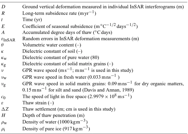
Table A1. Notation and constants.
D Ground vertical deformation measured in individual InSAR interferograms (m) R Long-term subsidence rate (m yr−1)
t Time (yr)
E Coefficient of seasonal subsidence (m◦C−1/2days−1/2) A Accumulated degree days of thaw (◦C days)
εInSAR Random errors in InSAR deformation measurements (m)
θ Volumetric water content (–) κ Dielectric constant of soil (–) κw Dielectric constant of pure water (80)
κg Dielectric constant of solid matrix grains (–)
ν GPR wave speed (m s−1; m ns−1is used in this study) νw GPR wave speed in fresh water (0.033 m ns−1)
νg GPR wave speed in solid matrix grains: 0.09 m ns−1for dry organic matters, 0.15 m ns−1for silt and sand (Davis and Annan, 1989)
c0 The speed of light in free space (2.9979×10⁸m s−1)
ε Thaw strain (–)
1Z Thaw settlement (m; cm is used in this study) H Depth of thaw penetration (m)
ρw Density of water (1000 kg m−3)