SRef-ID: 1607-7946/npg/2005-12-671 European Geosciences Union
© 2005 Author(s). This work is licensed under a Creative Commons License.
Nonlinear Processes
in Geophysics
Statistical properties of nonlinear one-dimensional wave fields
D. Chalikov
Earth System Science Interdisciplinary Center (ESSIC), University of Maryland, College Park, MD 20 742–2465, USA Received: 30 September 2004 – Revised: 31 January 2005 – Accepted: 21 March 2005 – Published: 30 June 2005
Abstract. A numerical model for long-term simulation of gravity surface waves is described. The model is designed as a component of a coupled Wave Boundary Layer/Sea Waves model, for investigation of small-scale dynamic and ther-modynamic interactions between the ocean and atmosphere. Statistical properties of nonlinear wave fields are investigated on a basis of direct hydrodynamical modeling of 1-D poten-tial periodic surface waves. The method is based on a non-stationary conformal surface-following coordinate transfor-mation; this approach reduces the principal equations of po-tential waves to two simple evolutionary equations for the el-evation and the velocity potential on the surface. The numer-ical scheme is based on a Fourier transform method. High accuracy was confirmed by validation of the nonstationary model against known solutions, and by comparison between the results obtained with different resolutions in the horizon-tal. The scheme allows reproduction of the propagation of steep Stokes waves for thousands of periods with very high accuracy. The method here developed is applied to simu-lation of the evolution of wave fields with large number of modes for many periods of dominant waves. The statistical characteristics of nonlinear wave fields for waves of different steepness were investigated: spectra, curtosis and skewness, dispersion relation, life time. The prime result is that wave field may be presented as a superposition of linear waves is valid only for small amplitudes. It is shown as well, that non-linear wave fields are rather a superposition of Stokes waves not linear waves.
Potential flow, free surface, conformal mapping, numeri-cal modeling of waves, gravity waves, Stokes waves, break-ing waves, freak waves, wind-wave interaction.
1 Introduction
One of the most important problems of geophysical fluid dy-namics is the interaction of wind waves and the atmospheric boundary layer. Until recently, the investigations of the ma-rine boundary layer were based on the standard theory of
Correspondence to: D. Chalikov
(dchalikov@essic.umd.edu)
a boundary layer above an infinite, flat, rigid surface (see review by Geernart, 1990). In fact, the presence of waves was considered a minor inconvenience forcing one to mod-ify the roughness parameter affecting the wind profile. How-ever, Wave Boundary Layer (WBL) has very specific proper-ties, created by the presence of multi-mode moving surface. Waves modify the basic dynamic and thermodynamic inter-actions of air and water and, as well, the exchange by gases. Investigation of the interaction of wind and waves is impor-tant for parameterizing of micro-scale ocean-atmosphere in-teraction for weather and wind waves forecasting, and for climate modeling. This problem has been intensively inves-tigated experimentally, theoretically, and numerically (see Chalikov, 1986; Donelan, 1990; Belcher and Hunt, 1998). All numerical investigations, based on Reynolds equations (begun by Gent and Taylor, 1976; Chalikov, 1978) were per-formed for 2-D turbulent flow above monochromatic waves, so they refer to an essentially steady motion. Application of monochromatic experimental and theoretical results for real nonlinear and multimode wave fields was based on a linear assumption. That is, all variables may be obtained by simple superposition of linear modes with different amplitudes. An evident extension of this monochromatic approach might be based on a multi-mode presentation of dispersive wave fields with preassigned spectrum S (see review Chalikov, 1986). Generally, however, this presentation is also incorrect: with increasing the resolution of spectrum 1k, the geometrical properties of surfaceηapproximated by relation
η=X(2Sk1k)1/2sin(kx−ωt ) (i)
surfaces based on the principal equations for potential mo-tion with an interface. Surely, actual sea waves are rotamo-tional. And they are affected by turbulence, because they are gener-ated, migrate, and break in a shifted drift flow. However, potential approximation describes the wave dynamics better than (i), because it is not sensitive to resolution in Fourier space. Even in potential approximation, the wave surface appears as a real physical object, whereas spectral presen-tation obscures its nonlinear nature. Actually, as resolution 1kincreases, the differentk-th modes assigned in the initial conditions do not move as separate wave modes with spe-cific dispersion relation: waves separated in a Fourier space join together, forming a superposition of nonlinear waves. The spectrum therefore describes a finite number of nonlin-ear waves rather than a continuous spectrum of linnonlin-ear waves. The experimental and simulated spectra appear continuous, because of the essential linearity of Fourier analysis and be-cause of the amplitudes of these discrete nonlinear waves change in time. Contrary to (i), the solution of the wave equa-tions converges with increasing spectral resolution (Chalikov and Sheinin, 1995), what proves the applicability of a such approach to the simulations of wind-wave interaction.
This study describes the results of numerical simulations of multi-mode wave fields based on a scheme developed by Chalikov and Sheinin (1996, 1998, 2005). The air/water model has been also completed (Chalikov, 1998); and nu-merical investigation of wind-wave interactive dynamics is underway. Because wave development of waves occurs at distances which are much larger than the length of the domi-nant wave, the periodic boundary conditions have been used. This assumption simplifies the construction of a numerical scheme, because it makes possible the application of the Fourier transform method. In this paper, we consider 1-D nonlinear waves only. The scheme here developed is exact, allowing simulating of waves for periods much longer than the period of the dominant wave.
The primary advantage of the potential approximation is that the system of Euler equations is reduced to the Laplace equation. However, the solution to the flow problem of sur-face wave motion is complicated by the required applica-tion of kinematics and dynamic boundary condiapplica-tions (both nonlinear) onto the free surface, the location of which is un-known at any given time,t.
Numerical simulation of surface waves has a long history. The most general approach to simulate a motion with a free surface is based on a marker and cell (MAC) method (Har-low and Welch, 1965). This approach assumes the tracing of a variable surface within a fixed grid with different order accuracy (for example, Noh and Woodward, 1976; Hirt and Nichols, 1981; Prosperetti and Jacobs, 1983; Miyata, 1986). Currently, the applicability of this method is restricted to sim-ulations over relatively short-term periods. Accuracy of this method will increase significantly, however, when very high resolution becomes possible. An advantage of this method is that it can be used for simulation of 3-D rotational mo-tion of viscous fluids even for non-single value interface. A motion with a single-value 1-D and 2-D interface is readily
simulated using the simplest surface-following coordinates (x, y, z−η(x, y)), where (x, y, z) are Cartesian coordinates andηis surface elevation (Chalikov, 1978). This system of coordinates is unsteady and non-orthogonal, so equations of motion become complicated. Still, this method has been ap-plied for the simulation of wave interaction with a shear flow (Dimas and Triantafyllou, 1994). Evidently, this approach may be combined with the MAC method, applied locally in the intervals with large steepness. Waves on finite depth have been investigated by transforming the volume occupied by fluid into a rectangular domain (Dommermuth et al., 1993). Much more complicated surface-following transformations have been constructed, including a case of a multiple-valued surface (Thompson et al., 1982). The grid method was gener-alized with adaptive grids (e.g. Fritts et al., 1988), and using a finite-volume approach (Farmer et al. (1993).
Fortunately, many observed properties of surface waves are reproduced well based on a a potential approach, which makes possible a reduction in dimensionality by one. The numerical methods for inviscid free-surface flow have been reviewed by Mei (1978), Yeung (1982), Hyman (1984), and for viscous flows by Floryan and Rassmussen (1989). The most recent review of numerical methods for incompress-ible nonlinear free-surface flow was presented by Tsai and Yue (1996). The scope of this review is limited to those works published after the last-mentioned review, which is devoted to free periodic waves and is based on the principal equation for potential waves.
allowing the model to reproduce sharpening and overturning waves. To increase stability, the authors applied very selec-tive smoothing. Dold (1991) noted, however, that the ad-vantage conferred by non-uniformity of the grid is absent for long-term integration. Wave sharpening results from nonlin-ear group effects, which generate a convergence of energy in physical space (Song and Banner, 2002), though is impossi-ble to predict the location of these events. Nonetheless, Hen-derson et al. (1999) demonstrated good results from long-term simulations of nonlinear evolution of wave field with an initially uniform grid.
Another group of numerical methods is based on tradi-tional perturbation expansions (often combined with Fourier transform method); in principle, these include arbitrary high orders of interactions (Watson and West, 1975; Dommer-muth and Yue, 1987; West et al., 1987). However, the num-ber of needed Fourier modes in this scheme multiplies with increasing steepness. Indeed, this method becomes inappli-cable when waves approach overturning. Modification of the high-order spectral method was suggested by Fenton and Rienecker (1982).
Craig and Sulem (1993) improved stability by using the expansion for vertical velocity instead of potential. This method was later generalized for 2-D potential waves (Bate-man et al., 2001). A numerical scheme for 1-D potential waves, based on non-orthogonal surface-following coordi-nate system and Fourier transform, was developed by Cha-likov and Liberman (1991). The method is based on iterative transfer of the potential from a fixed coordinate system onto free surface; it was used to simulate the bound waves dy-namics observed by Yuen and Lake (1982). This method is also applicable to 2-D potential waves; however, it be-comes ineffective for large numbers of modes with highly variant amplitudes (also true for many methods based on ex-pansions). The reason for this limitation restriction: the small waves overrun the surfaces of large waves. The amplitudes of wave disturbances with large wave numbers attenuate with depth quickly, becoming insignificant for the depth of domi-nant wave height (Zhang et al., 1993). In this case, restoring the high-order modes on a free surface becomes inaccurate. Still, the high- order perturbation methods (and all methods based on the surface-following coordinates) represent a huge advance over quasi-linear theories based on small-amplitude assumption.
A numerical scheme for direct hydrodynamical model-ing of 1-D nonlinear gravity and gravity-capillary periodic waves was developed by Chalikov and Sheinin (1996, 1998). This scheme is based on conformal mapping of a finite-depth water domain. For the stationary problem, this map-ping represents the classical complex variable method (e.g. Crapper, 1957, 1984) originally developed by Stokes (1847). In a stationary problem, this method employs the velocity potential 8and the stream function 9 as the independent variables. A nonstationary conformal mapping was intro-duced also by Whitney (1971), then considered by Kano and Nishida (1979) and by Fornberg (1980). Tanveer (1991, 1993) used this approach for investigating Rayleigh-Taylor
instability and the generation of surface singularities. A new way of deriving equations, a description of a numerical scheme (and its validation) as well as the results of long-term simulations were presented at ONR meeting held in Arizona in 1994 (Sheinin, Chalikov, 1994). Later, this scheme was described in detail by Chalikov and Sheinin (1996; 1998) and in Sheinin and Chalikov (2000). The ChSh numerical ap-proach is based on nonstationary conformal mapping for fi-nite depth. This allows rewriting of the principal equations of potential flow with a free surface in a surface-following coor-dinate system. The Laplace equation retains its form, and the boundaries of the flow domain (i.e. the free surface and, in the case of finite depth, the bottom) are coordinate surfaces in the new coordinate system. Accordingly, the velocity po-tential in the entire domain receives a standard representa-tion based on its Fourier expansion on the free surface. As a result, the hydrodynamical system (without any simplifi-cations) is represented by two relatively simple evolutionary equations that can be solved numerically in a straightforward way. The advantages of this approach were briefly discussed by Dyachenko et al. (1996); later, the method was used by Zakharov et al. (2002) to demonstrate the nonlinear proper-ties of steep waves. In principle, the ChSh method is similar to method developed by Meiron et al. (1981). They con-cluded that this method is applicable only to “moderately distorted geometry”. For simulations of the Stokes wave with peak-to-trough amplitude at 80% of the theoretical max-imum, they found that “time stepping errors can cause modu-lation of the steady waves for times longer thant=4π” (time is normalized with the length scale and gravity acceleration). Our scheme, in contrast, allows simulation of the propaga-tion of Stokes wave with amplitude at 98% of the maxi-mum for hundreds of periods (and much longer) without no-ticeable distortions (see Fig. 1, below). Because Meiron et al. (1981) used the same accuracy time-stepping scheme as the 4th order Runge-Kutta scheme applied here, we conclude that their errors were generated simply by low resolution: for an approximation of Stokes wave profile onlyN=64 points were used. We exploited thousands of points. (Zakharov et al. (2002) used up to one million Fourier modes). Impre-cise approximation of the initial shape of a Stokes wave also might result in instability. The stability of Stokes wave de-pends largely on the degree of truncation of the Fourier series used to describe the wave. This effect is better pronounced for large steepness. For example, for the case a=0.42 (half of crest-to-trough height), the Stokes wave initially assigned by five modes (with resolution 2000 modes, 8000 grid points) collapses to time t=1. Exact Stokes wave (assigned by the hundreds of modes) runs stably for the same resolution the thousands of periods.
Fig. 1. Long-term evolution of amplitudes of the first 880
con-stituents of the Stokes waves: (ak=0.42; each 10th concon-stituents is shown) during 2 686 500 time steps (932 periods).
of sharp crests. Formally, conformal mapping exists up to the moment when an overturning volume of water touches the surface (Dyachenko, 2004, personal communication). In such an evolution, the number of Fourier modes needed in-creases very quickly. If the special measures (smoothing) are not taken, the calculations typically terminate much earlier, due to strong crest instability (Longuet-Higgins, 1996) mani-fested by splitting of the falling volume into two phases. This phenomenon is obviously non-potential. Hence, as in many branches of geophysical fluid dynamics, special measures must be taken to prevent numerical instabilities while con-currently accounting on the physical consequences of these events.
Our method is applied to the simulation of wave fields represented in initial conditions by superposition of running waves with random phases assigned by linear theory. We show that wave fields lose their initial structure and soon de-velop new, specific features. These become pronounced the larger the nonlinearity of the initial state. Of course, this de-veloping of waves influences significantly the air flow above wave surface.
2 Equations
Consider the principal 2-D equations for potential waves written in Cartesian coordinates, i.e. the Laplace equation for the velocity potential8
8xx+8zz=0, (1)
and the two boundary conditions at the free surface h=h(x, t ): the kinematic condition
ht+hx8x−8z=0, (2)
and the Lagrange integral
8t+12(82x+82z)+h+pe−σ hxx(1+h2x) −3
2 =0, (3) wherepeis the external surface pressure. (Independent
vari-ables in subscripts denote partial differentiation with respect to these variables.)
The equations are to be solved in the domain
− ∞< x <∞ −H ≤z≤h(x, t ), (4) whereH is either a finite depth or infinity. The variables8 andhare considered to be periodic with respect tox: 8(x+2π, z, t )=8(x, z, t ) h(x+2π, t )=h(x, t ), (5) and a normal velocity condition at the bottom is assumed to be zero:
8z(x, z= −H, t )=0 (6)
Equations (1)−(3) are written in the nondimensional form with the following scales: lengthL, where 2π Lis the (di-mensional) period in the horizontal, timeL1/2g−1/2and the velocity potentialL3/2g−1/2 (g is the acceleration of grav-ity). Pressure is taken to be normalized by water density (so its scale is Lg). The last term in Eq. (3) describes the effect of surface tension, and
σ = 0 gL2
is a nondimensional parameter (0≈8·10−5m3s−2is the kine-matic coefficient of surface tension for water).
System in Eqs. (1)−(6) is solved as an initial-value prob-lem for the unknown functions8andh,with initial condi-tions8(x, z=h(x, t=0), t=0) andh(x, t = 0). Note that although Eqs. (2) and (3) are for the free surface, there are no straightforward ways to reduce the problem to a 1-D because, to evaluate8z, one has to solve the Laplace equation (1) in
the domain (4) with a curvilinear upper boundary that may be any function ofx. This difficulty is known to render inte-gration of the system in Cartesian coordinates either insuffi-ciently accurate or too expensive computationally (Chalikov and Liberman, 1991). So, for time periods much greater than the time scale, it is quite impractical.
To realize a feasible numerical solution, we introduce a time-dependent surface-following coordinate system that conformally maps the original domain (4) onto the strip
− ∞< ξ <∞ − ˜H ≤ζ <0 (7) with a periodicity condition given as
x(ξ, ζ, τ )=x(ξ+2π, ζ, τ )+2π,
z(ξ, ζ, τ )=z(ξ+2π, ζ, τ ), (8) whereτ is the new time coordinateτ=t.
According to complex variable calculus, conformal map-ping(7)→(4)exists and is unique up to an additive constant forx. Note that for the stationary problem, this mapping rep-resents the classic complex variable method (e.g. Crapper, 1984) originally developed by Stokes (1847).
Due to periodicity condition (8), the required conformal mapping can be represented by the Fourier series:
x=ξ+x0(τ )+
X
−M≤k<M,k6=0
η−k(τ )
coshk(ς+ ˜H )
z=ζ+η0(τ )+
X
−M≤k<M,k6=0
ηk(τ )
sinhk(ς+ ˜H )
sinhkH˜ ϑk(ξ ), (10) whereηkare the coefficients of Fourier expansion of the free
surfaceη(ξ, τ )with respect to the new horizontal coordinate ξ:
η(ξ, τ )=h(x(ξ, ζ =0, τ ), t=τ )= X −M≤k≤M
ηk(τ )ϑk(ξ ), (11)
ϑkdenotes the functions
ϑk(ξ )=
coskξ, k≥0
sinkξ, k <0 ; (12) Mis the truncation number (so farM=∞is assumed);x0(τ )
can be chosen arbitrarily, though it is convenient to assume thatx0(τ )=0.
Nontraditional presentation of the Fourier transform with definition (12) is, in fact, more convenient for calculations because (ϑk)ξ=kϑ−kand P(Akϑk)ξ=−PkA−kϑk. So
the Fourier coefficientsAkform the arrayA(−M:M), thus
making possible a compact programming in Fortran90. The lower boundaryζ=−∼H can not be chosen arbitrar-ily, since the relation
z(ξ, ζ = − ˜H , τ )= −H (13) must hold; after substituting expansion (10), (13) yields:
˜
H=H+η0(τ ) . (14)
Sinceη0is determined by the Fourier expansion (11), and,
generally, is an unknown function of time, H˜ also is time-dependent. Note that the definition of both coordinatesξ and ζis based on Fourier coefficients for surface elevation. It fol-lows then from (9) and (10), that the time derivativeszτand
xτ for Fourier components are connected by the simple
rela-tion
(xτ)k=(zτ)−kcoth(kH ),˜ (15)
Due to conformity of the mapping, Laplace equation (1) re-tains its form in(ξ, ζ )coordinates. It is shown in ChSh that the system (1) – (3) can be written in the new coordinates as follows:
8ξ ξ+8ζ ζ =0 (16)
zτ =xξg+zξf (17)
8τ =f 8ξ−12J−1(82ξ−82ζ)−z−pe+
σ J−3/2(−xξ ξzξ+zξ ξxξ), (18)
where (17) and (18) are written for the surfaceζ=0 (so that z=η, as represented by expansion (11)),J is the Jacobian of the transformation
J =xξ2+z2ξ =x2ζ+z2ζ, (19) g=(J−18ζ)ζ=0; (20)
andf is a generalization of the Hilbert transform ofg, which fork6=0 may be defined in Fourier space as
fk =g−kcothkH ,˜ (21)
following in fact from Eq. (15).
Boundary condition (6) is rewritten as
8ζ(ξ, ζ = − ˜H, τ )=0 . (22)
The solution to the Laplace equation (16) with boundary con-dition (22) is readily yields to Fourier expansion, which re-duces the system (16)−(18) to a 1-D problem:
8= X −M≤k≤M
φk(τ )
coshk(ζ+ ∼H )
coshk∼H ϑk(ξ ), (23) where φk are Fourier coefficients of the surface potential
8(ξ, ζ=0, τ ). Thus, Eqs. (17), (18), and (20) constitute a closed system of prognostic equations for the surface func-tionsz(ξ, ζ=0, τ )=η(ξ, τ )and8(ξ, ζ=0, τ ). It may also be regarded as a system of ordinary differential equations for the Fourier coefficientsηk, φk. Its explicit form would be
some-what complicated; however, it is not needed. As described in the next section, we use the Fourier transform method to cal-culate the nonlinearities. Indeed, the transform method may be called an exact method if the order of nonlinearity is finite. Otherwise, the accuracy of the method should be established empirically.
Thus, the original system of Eqs. (1)−(3) is transformed into two evolutionary Eqs. (17) and (18) which are written for the free surface and, thus, are essentially 1-D (both spa-tial derivatives of8are obtained by differentiating the series (23)) and can be solved using the Fourier transform method (see next Sect. 3 and also ChSh).
For deep water (H=∞), the coefficients in expansions (9), (10) and (23) become simpler. The domain (7) turns into the semi-planeζ <0(z→−∞whenς→−∞, a condition which replaces (14)); and the conformal mapping (9) and (10) ac-quires the form
x=ξ +x0(τ )+
X
−M≤k<M,k6=0
η−k(τ )exp(kζ )ϑk(ξ ), (24)
z=ζ+η0(τ )+
X
−M≤k<M,k6=0
ηk(τ )exp(kζ )ϑk(ξ ); (25)
and the solution (23) of the Laplace equation (16) reduces to 8= X
−M≤k≤M
φk(τ )exp(kζ )ϑk(ξ ); (26)
In the absence of capillarity, the upper boundary condition is p=pe. All model simulations presented herein hold the
pre-scribed external surface pressure constant. One may there-fore assume
The lower boundary condition readily follows from the La-grange integral, written for the bottom in the (nondimen-sional) Cartesian coordinates: pz=−1. So, in the new
co-ordinates we have
zζpζ = −J at ζ = − ˜H . (28)
For deep water, this condition becomes
pζ → −1 at ζ → −∞. (29)
3 Numerical scheme and its accuracy
For spatial approximation of system (32) and (33) we use a Galerkin-type (or “spectral”) method based on a Fourier ex-pansion of the prognostic variables with a finite truncation numberM. The problem is thus reduced to a system of ordi-nary differential equations for 4M+2 Fourier coefficients ηk(τ ), φk(τ ),−M≤k≤M:
˙
ηk=Ek(η−M, η−M+1, ..., ηM, φ−M, φ−M+1, ..., φM) (30)
˙
φk =Fk(η−M, η−M+1, ..., ηM, φ−M, φ−M+1, ..., φM) (31)
whereEk, Fk are, respectively, the Fourier expansion
coeffi-cients for the right-hand sides of Eqs. (17) and (18) as func-tions ofξ.
To calculate Ek, Fk as functions of the prognostic
vari-ablesηk, φk, differentiation of the Fourier series is used (the
spatial derivatives are thus evaluated exactly) and the nonlin-earities are calculated with the so-called transform method (Orszag, 1970; Eliassen et al.., 1970), by their evaluation on a spatial grid. IfY (u(ξ ), v(ξ ), w(ξ ), ...) is a nonlinear function of its arguments represented by their Fourier ex-pansions, grid-point valuesu(ξj),v(ξj),w(ξj),. . . are first
calculated (in other words, inverse Fourier transforms are performed).Then Y(j )=Y (u(ξ(j )), v(ξ(j )), w(ξ(j )), ...) are evaluated at each grid point. Finally, the Fourier coefficients Ykof the functionY are found by a direct Fourier transform.
Here ξ(j )=2π(j−1)/N−N is the number of grid-points. This approach is largely exploited extensively in geophysical hydrodynamics, in global atmospheric modeling particularly. For the method to be a purely Galerkin one, that is, to ensure the minimum mean square approximation error, the Fourier coefficients Ek, Fk must be evaluated exactly for
−M≤k≤M. For this purpose, one must choose
N > (ν+1)M (32)
whereν is the maximum order of nonlinearities. Since the right-hand sides of Eqs. (17) and (18) include division by the Jacobian, the nonlinearity is of infinite order such that the above condition onN can not be met. However, numerical integrations show that if one chooses a value ofN ensuring exact evaluation of cubic nonlinearities (ν=3 in Eq. (32)), a further increase in N (with a fixedM) does not affect the numerical solution. For the results presented in Section 5, N=4Mwas chosen.
However high the spectral resolution might be, long-term simulations of strongly nonlinear waves require that the en-ergy flux be parameterized into the severed part of the spec-trum (|k|>M). If ignored, spurious energy accumulations at large wave numbers can corrupt the numerical solution. Sim-ple dissipation terms were therefore added to the right-hand sides of Eqs. (43) and (44):
˙
ηk=Ek−µkηk (33)
˙
φk=Fk−µkφk (34)
with µk =
(
rM
| k|−kd
M−kd
2
if|k|> kd
0 ot herwise
(35)
where kd=M/2 and r=0.25 were chosen for all runs
dis-cussed below. We found the sensitivity of the results to rea-sonable variations of kd and r to be low. The dissipation
effectively absorbs energy at wave numbers close to the trun-cation numberMwhile leaving longer waves virtually intact and as well as modes with wave numbers|k| ≤kdunaffected.
Note that an increase of the truncation numberMshifts the dissipation area to higher wave numbers (and, withM→∞, the energy sink due to dissipation tends to zero). Therefore, the scheme with the dissipation incorporated retains an ap-proximation of the original (non-dissipative) system.
For time integration, the fourth-order Runge-Kutta scheme was used. The choice of time step was done empirically. For example, for M=100, a time step was equal to 0.01. For M=1000, it was 0.002. Increasing local steepness and surface curvature often forces to apply smaller time steps. Capillarity effects were not included in this study. If these are taken into account, the restrictions on time step become more severe (ChSh).
A separate problem is initial data normally given in the Cartesian coordinates. These need to be converted to the (ξ, ζ )coordinates. For this purpose, and for processing of the results, an algorithm based on the periodic high-order spline functions has been developed. The algorithm carries out the transformation with computer accuracy.
gravity waves for deep water was described in detail in ChSh (Sect. 3). The results for the case of finite depth were ob-tained in Sheinin and Chalikov (2000). These solutions (as well as Crapper’s waves) may be considered exact. They were used for validation of the nonstationary model (system Eqs. (16)−(18)).
Discussion of long-term validation runs is found in ChSh. The model was validated against the three types of waves: pure capillary deep-water (Crapper’s) waves (analytical so-lutions), pure gravity, and also gravity-capillary waves, the latter obtained numerically with the algorithm referred to above. For all test cases, visual comparison of instantaneous wave profiles showed that the waves moved with no any spu-rious perturbations. To estimate “steadiness” of the numeri-cal solution quantitatively, we numeri-calculated the phase velocities and amplitudes of the Fourier components for consecutive moments of time, and obtained their temporal means and standard deviations over the period of integration. Results in ChSh (Table 4) show that even for steep waves the calcu-lated phase velocities were very close to their exact values (i.e. those obtained for the stationary solutions) for all three types of waves. Conservation of the amplitudes was also very accurate: deviations during the simulations from initial values were always less than 10−7for the Stokes wave, and less than 10−11for the capillary and gravity-capillary waves. The modes retained their initial energies and remained con-sistent in phase; consequently, the simulated waves did not change their shapes during the integration. This confirms that these waves are stable with respect to truncation errors, and also that the numerical solutions approximate the solutions of the original differential equations with high accuracy. For all model simulations described in (Chalikov and Sheinin, 2005), differences between the solutions presented and their versions obtained withMtwice as large were nearly absent, confirming a convergence of numerical scheme.
Additional validation was performed by simulating of very steep Stokes waves for ak=0.42 (M=1000, 1τ=0.0025). The evolution of first 880 amplitudes is shown in Fig. 1. This boring picture shows that amplitudes, and, consequently, the shape of Stokes wave remained unchanged with very high accuracy. These integrations can be continued much longer without of noticeable changes in amplitudes. After 2 686 500 time steps (932 periods), the total energy forak=0.42 and M=1000 decreased merely at 3·10−8%. The analogous cal-culations for ak=0.42 performed by Dold (1992) quickly collapsed due to numerical instability. Exact phase veloc-ity of Stokes waves with ak=0.42, obtained for the stationary solution is 1.089578. Direct calculation of phase velocity of simulated Stokes wave gave value 1.089579±10−6.
Note that validation based on simulation of running Stokes waves is complete and not trivial, because nonstationary equations “do not know” the stationary solution obtained in a moving coordinate system via a different method. However, the results shown in Fig. 1 were obtained for demonstration of accuracy of scheme only. High stability of steep Stokes wave was determined by its position in a Fourier space: the modes were connected with wave numbersk=1, 2, 3. . .M.
So, all Fourier modes were the modes of Stokes wave, and there was no room for developing of an instability. Another situation takes place when the modes of the Stokes wave are the Fourier modes withk=n, 2n, 3n. . .M (nis any integer number), and the intermediate modes in initial conditions equal to zero. In this case, the errors of approximation can initiate the Benjamin-Feir instability (Benjamin, Feir, 1967), and a train of the Stokes waves can loose its initial shape or come to breaking instability (if steepness is large). This phenomenon is a subject of forthcoming paper.
Remarkably, conformal mapping made possible a repro-duction of the essential stages of the breaking process when the surface ceases to be a single-valued function (Chalikov and Sheinin, 2005). This initial stage of wave breaking ex-hibits a sharp jet originating from a wave crest. The inte-gration in this case is always terminated; but due to high accuracy of the scheme, however, the numerical and phys-ical instabilities follow each other very closely. Two ways of treating breaking were exploited. When breaking is the sub-ject of investigation, it is simulated explicitly to the point of instability. (The last, unrealistic phase of breaking is easily eliminated from consideration of the energy conservation.) The final stage of breaking is evidently a non-potential phe-nomenon. This direct method is inapplicable when used for long-term simulation of the evolution of multi-mode wave fields and, for modeling of wave/wind interactions (Chalikov, 1998). For these reasons we developed a method of parame-terization of breaking effects based on a high-order selective smoothing (Chalikov, Sheinin, 2005). However, in calcula-tions considered here, we did not use this parameterization; all cases in which breaking instability took place were simply excluded from consideration.
4 Statistical properties of wave field
In this study, we applied the method for numerical simulation of surface waves developed in ChSh to investigation of sta-tistical properties of nonlinear wave fields. Generally, this in-vestigation confronts complications associated with specific wave instability – wave breaking. If initial wave energy is large, the onset of wave breaking leads inevitably to termi-nation of calculations. Still, this instability can be eliminated with algorithms of breaking parameterization. If such algo-rithms are applied, however, the statistics of free waves can be distorted. For example, this smoothing algorithm elimi-nates the appearance of high, sharp waves.
Therefore, we first investigated the dependence of time to the onset of wave breaking on the initial conditions. The appropriate integral characteristics for fixed length scale might be the initial energy. For different length scales, this characteristic is incomplete. More appropriate is the initial steepness of surfaces:
s∝
M Z
0
k2S(k)dk
1 2
Fig. 2. Dependence of time to onset of breaking instability on rms
steepnesss. Dotted line is approximation Eq. (39)
Initial conditions were assigned as superposition of linear waves with amplitudes
ak = (
a0
k k0
−m
k0≤k≤kd.
0 ot herwise.
(37)
and random (different for each case) sets of phases. The mode with wave number k0 has amplitude a0, with
ampli-tudes abovek0decreasing as k−m. The value ofk0defines
the resolution of the spectrum, so it cannot be too small. In most calculations,k0=10 andm=6 were chosen. Further
in-creases ofk0did not change the results, which are described
below. The statistical results were also very close whenm=5 was chosen. Because the steepnesssfor steep (but not yet breaking) waves decreases slightly during long-time simula-tions (due to tail dissipation (33)-(35)), the effective steep-ness for each run was obtained by averaging over time. The number of modesMwas 400, with grid pointsN=1600, time step1τ=0.0025. Calculations were performed for 70 cases al =0.09+0.001·l, l=1,2,3...70 (38)
Onset of breaking was recognized when total energy started growing then exceeded its initial value by 1%. This criteria specifies time of breaking onset with high accuracy, because the 4th order Runge-Kutta scheme develops instability very quickly. The onset of breaking depends not only on total nonlinearity of the initial wave field but, as well, on the ini-tial set of phases. However, this dependence is much weaker than the dependence on steepness. To incorporate the effect of initial phases, the calculations Eq. (38) were repeated with different sets of phases. Total number of runs: 980. The de-pendence of time to breakingTl(timeτnormalized by period
of peak waveTp=2π/
√
k0)on effective steepness is
demon-strated in Fig. 2. Each point was obtained by averaging over the sampling set with a total length of 160 000 values (100 wave profiles).
As we show, the stability of a wave field and its exis-tence without breaking decreases quickly with increasing the
steepness. For large initial steepness of the order of 1, break-ing occurs immediately and dependence on initial phases be-comes much more significant. However, for effective steep-nesssless than 0.11 the breaking was virtually absent. This statement can not be considered as an unequivocal. Still, our results confirm that breaking onset below s=0.10 in runs up to t=2,500 was not observed. The dependence ofTkonsmay
be approximated by the formula
Tk =4.6·10−4s−5.61, (39)
Approximation (39) has a right asymptotic behavior (Tk→∞
ats→0); it is unlikely that the specific form of this depen-dence is correct for values ofssmaller than here explored. The number of modes used in our calculations was, much larger than in calculations made by Song and Banner (2002), but a value of threshold for onset of breaking s=0.10 is close to that in their paper.
For calculations of statistical characteristics of waves, the 10 long-term runs were performed up to 1 000 000 time steps (790 periods of peak wave) with initial peak steepness in the range of a0k0=0.0001÷0.09, corresponding to an
ef-fective steepness in the ranges=0.0001÷0.106.The num-ber of modes M for the cases 1÷7 was 400, the number of grid points N=1600, time step was 0.0025. For cases 8÷10 (corresponding to large steepness), the tail dissipation Eqs. (33)−(35) for M=400 was large. To reduce this ef-fect, the number of modes for these cases was increased to M=1000 (N=4000), although time step and the number of steps were the same as for M=400. The amplitudesakand
corresponding effective steepness are outlined in Table 1. The wave spectra and rate of dissipation are represented in Fig. 3. The high wave-number part of spectrum fluctu-ates within the range of its averaged values, the amplitudes of these fluctuations grow with increasing of initial steepness and wave number. Gray areas in right part of the frames cor-respond to the tail dissipation function (See Eq. 35). Dk=µk
z2k+z2−k (40) Tail dissipation is located in the high- frequency part of the spectrum. It removes the fast growing but very small modes in a vicinity of the cut wave numberM. This dissipation is so weak that it does not influence significantly the con-servation of total energy. For the cases 1÷7, the energy de-creases during a period of integration in 10th decimal digits; for the steepest initial conditions (case 10) the energy de-creased at 10−3%. Generally, the accuracy of conservation
Table 1. Parameters of numerical experiments.
# 1 2 3 4 5 6 7 8 9 10
a0 0.00001 0.001 0.002 0.003 0.004 0.005 0.006 0.007 0.008 0.009 s 0.0001 0.013 0.026 0.029 0.039 0.052 0.079 0.089 0.099 0.106
M 400 400 400 400 400 400 400 1000 1000 1000
Fig. 3. Averaged for t=2500 (790 wave-peak periods) wave spectra, initially assigned by Eq. (37). The curves in the right side of each panel
are rates of dissipation of potential energy (Eq. (40)). Straight line corresponds toS=k−6function. The grey vertical bars are the scatter of the rms of the spectra, and the rate of dissipation.
form=5 andkd=10. As will be shown below, fast
adjust-ment of the spectrum to its quasi-equilibrium shape is due to a strong nonlinearity, which makes the time scales for the individual high wave-number components very short.
Fast modification of the wave field due to nonlinearity is clearly seen in Fig. 4, in which the long-time evolution of the amplitudes of the first six components (with the wave num-bersk=10÷15)for different rms steepness are given. Only for extremely flat waves with rms steepness of the order of 10−4, the wave amplitudes remain constant over a long time. For the rms steepnessak=0.013, the 15th amplitude fluc-tuates significantly. With increasing steepness these fluctu-ations spread between all modes in a spectral peak, further
Fig. 4. Evolution of five consequent amplitudes starting from peak wave numberk=10 for different steepness during 790 peak periods.
It is useful to consider the time scaleTl, characterizing the
typical “life time” of the wave components
Tk=Ep
k12 2π
∂E
p
∂t
2! −1
2
, (41)
whereEp=12 h2k+h2−k
is the potential energy ofk−th wave component in the Cartesian coordinate system. Time scale Tk is normalized by the period of linear wave component
2π k1/2. Dependences ofTk on the wave numbers for
dif-ferent rms steepness are given in Fig. 5, together with their scatter. Again, all wave components are stable for very small steepness only: their amplitudes remains constant over hun-dreds, even a thousand of periods. As frequency increases, time scale Tk near the wave peak decreases up to 100 for
s=0.026, then up to 10 for s=0.106. For k>20, the time scales are very small (of the order of one period of linear wave with the same wave number) for all steepness consid-ered. An exception is the case withs=10−4. The spectral energy of wave components fork=20 is smaller at three dec-imal orders than in a wave peak. Evidently, such transient fluctuations cannot be attributed to the free surface waves, rather to wave turbulence (Zakharov, et al., 2004; Dyachenko et al., 2004).
This result becomes more evident if one considers the phase velocities of waves. One way to calculate an instanta-neous value of the phase velocity of the k-th wave component can be done with the relation
ck=
z−k∂z∂τk −zk∂z∂τ−k
k z2k+z−2k , (42)
where the derivatives on time are just right side of equation (17) written for Fourier components ofz. It is convenient to use Eq. (42) for calculations by the rms method
ck=
AD
D2, (43)
(ckis a mean phase velocity, A is the numerator and D is the
denominator in (42)), and rms of phase velocityck
crms=
(ck−ck)2 12
Fig. 5. “Life time” of the components of the wave field∼Tkexpressed in periods for every specific component (Eq. (41); solid lines). Grey
lines indicate the scatter of∼Tk. Dotted lines are the averaged wave spectrum. The numbers in the right upper corner are the effective
steepness.
linear dispersion relationck=k−1/2is perfectly accurate only
fors=0.0001. For waves with s=0.013, the fluctuations of phase velocity fork=20 become noticeable. Further increase of steepness increases the phase velocity of the high modes and its fluctuations grow. A simple explanation of these phe-nomena was given in ChSh. In fact, at each wave num-ber several modes coexist: one a free wave, others so-called “bound waves” corresponding the additional modes attached for every steep enough wave. The calculation of phase ve-locity based on Eqs. (42) and (43) gives a weighted value between the velocities of free and several bound modes. A separation of bound waves and free waves was conducted in ShCh by calculation a wave number-frequency spectrum. Bound waves are attributed to different carrying waves, so some have identical wave numbers. The amplitudes of car-rying waves change in time, due to nonlinearity (see Fig. 4), so a situation becomes very complicated. In order to under-stand how shape of wave differs from what it is assumed in linear theory, calculations of high-order moments for differ-ent steepness were performed.
The functionz(ξ )was transferred from conformal coordi-nates to function η(x) in Cartesian coordinates, using 4th order periodic polynomial spline (providing an accuracy of the order of 10−11)and then recorded for processing. Every hundred such records were linked in single set with length of L=160,000, which then was used for calculation of statis-tical characteristics: meanη; varianceV; skewnessS; and curtosisK:
η=1 L
L−1
X
j=0
ηj,V=
1 L−1
L−1
X
j=0
ηj−η
2
,S=1 L
L−1
X
j=0
η j−η
√ V
3
,
K=1 L
L−1
X
j=0
η j−η
√ V
4
−3, (45)
Fig. 6. Phase velocities of wave components as function of wave number (see Eq. (43)). Dashed line is a linear dispersion relation. Grey
vertical bars correspond to rms of phase velocities (Eq. (44)). Dotted line is a wave spectrum (right axis).
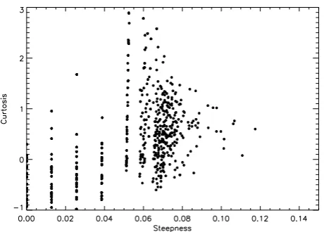
larger than the negative values, then S>0. Curtosis is positive if the crests are sharper and the troughs are smoother than in a case of linear waves. As seen in Fig. 7, the skewness is very close to zero for s=0.001 only; with increasing nonlin-earity it grows rapidly and reaches as large a value as S=0.35 – corresponding to significant exceeding of heights of crests over depth of troughs. Qualitatively, these properties are sup-ported by data on curtosis (Fig. 8) growing with increasing nonlinearity, and confirming that wave crests become sharper and troughs more gentle for steep waves.
Data on skewness and curtosis (Figs. 7 and 8), observa-tions of wave height records as well as the results of sim-ulations based on principal wave equations (as in Fig. 12) always exhibit the fundamental properties of nonlinear wave fields: the waves tend to be sharper and higher than harmonic waves.
A question arise: do the Stokes waves posses any prac-tical utility or they are simply example of an analyprac-tical so-lution for stationary gravity waves – waves so unstable that they never exist? Does a routine Fourier presentation used in most of theoretical and experimental investigations miss the nonlinear nature of steep waves?
Attempting to answer, a presentation of nonlinear wave field as superposition of Stokes waves was tried. Naturally
the functionsSk corresponding to the Stokes waves are not
orthogonal, so calculation of coefficients in expansion
h(x)=
M X
o
σkSk(σk) (46)
converts to minimization problem. Because the shape of Stokes wavesSkdepends on its amplitudeσk, this is a
non-linear problem – complicated but still resolvable. However, a more elegant solution was found.
Let us to consider the conformal coordinates for upper do-mainz>η.
x=ξa−
X
−M≤k≤M,k6=0
ν−k(τ )
coshk([Ha]−ςa)
sinhkH ϑk(ξa)
z=ζa+
X
−M≤k≤M,k6=0
ν−k(τ )
sinhk([Ha]−ςa)
sinhkH ϑk(ξa) (47) where νk are the Fourier coefficients of presentation of the
interface,ξa, ζa are the conformal coordinates in upper
Fig. 7. Skewness of wave field as a function of the effective
steep-ness (Eq. (45) third formula). Each point is obtained by averaging over a sampling set with total length of 160 000 values (100 wave profiles).
Fig. 8. The same as in Fig. 7, but for Curtosis of wave field (Eq. (45), forth formula).
is small. The opposite applies for the troughs. The system of coordinates Eq. (47) is used now for modeling of turbu-lent flow above waves and wind-wave interactions (Chalikov, 1998). In this paper, however, the first formula of Eq. (47) is used for introducing dependenceξa(ξ )for infinite heightHa.
An advantage of this transformation is that for the same ac-curacy of approximation the sharp waves in the lower coordi-nate need more of modes than in the upper coordicoordi-nates. The number of modes for the approximation with the same accu-racy in Cartesian coordinates lies somewhere between. This statement is illustrated in Fig. 9, representing the spectrum of Stokes waves with steepnessak=0.42 andak=0.43 (for infinite depths) calculated in the lower coordinates with the method ChSh. These solutions were transferred in the Carte-sian and upper coordinates with an accuracy of the order of 10−11. The convergence of Fourier expansion is fastest in the upper coordinates, and lowest in a lower coordinates. For k=10, the value of Fourier mode in upper coordinates is two
Fig. 9. Spectra of Stokes waves: (1) – in lower coordinates; (2)
– in Cartesian coordinates; (3) – in upper coordinate. Thin lines correspond to ak=0.42, thick lines to ak=0.43.
Fig. 10. Profiles of Stokes waves in Cartesian coordinates for ak=0.05, 0.10, 0.15, 0.20, 0.25, 0.30, 0.35 (k=1, solid lines). Dashed curves correspond toacos(kθ )(see Eqs. (47)).
decimal orders smaller than in Cartesian coordinates and by three decimal orders than in lower coordinates.
It is reasonable to consider what shape obtains the single modeacos(ξa)in upper coordinate transferred to Cartesian
Fig. 11. Upper panel – the same as in Fig. 3 spectra in linear
k-scale; Lower panel – difference between spectra and “spectrum” over Stokes waves.
weights corresponding to the inverse Jacobian of conformal mapping to upper coordinates. The left panel in Fig. 11 rep-resents the averaged wave spectra calculated in Cartesian co-ordinates for ten cases (Table 1), and the bottom panel is the difference between averaged wave “spectrum” in upper co-ordinates and spectrum in Cartesian coco-ordinates. Plainly, the difference at low wave numbers is large and positive, in high
wave numbers negative. This means that representation of a surface as a superposition of Stokes waves is more compact than routine representation as superposition of linear waves. It is well known that sea waves usually have sharp crests and gentle roughs. All quasi-linear theories ignore this evident property of actual wave fields. This reality explains, qual-itatively, the increasing the skewness and curtosis for steep waves shown in Figs. 7 and 8.
Visual observations of long-term evolution of wave sur-face shows that steep enough wave fields has quasi-periodic behavior: a period of more or less smooth waves followed by period when large waves becoming sharper (the same ef-fect as observed by Song and Banner, 2002). In our calcula-tions, the length of domain was equal to ten lengths of peak wave. During the period of sharpening, the several waves may become sharper simultaneously; more often, however, only one wave become sharper. In Fig. 12 (panel 1), the evo-lution of kinetic and potential energies for s=0.089 is given. Both energies fluctuate with amplitude up to 10%, their sum remains constant within many decimal digits. In panel 2, the top curve represents the evolution of the maximum wave height defined over whole period for 2,500 wave profiles sep-arated by interval1t=1; the bottom curve depicts evolution of the minimum value of the second derivative∂2η/dx2for the same set. The intervals of increasing wave height always coincide with minimums for the second derivatives, corre-sponding to sharpening of crests. In panel 3, the “sharpest” wave profile for time t=815 (corresponding the minimum of ∂2η/dx2)is drawn (dotted curve); solid line is the smoothest wave profile (minimum of absolute value of∂2η/dx2). Both profiles are equally smooth, except that the first has single high peak. The wave-number spectra of these profiles are given in panel 4. The spectrum corresponding to the first case has much larger high wave-number values. All these components were needed for correct approximation of a in-gle sharp peak in a domain. In sum, for large number of cases for developed wave fields a considerable part of high frequency does not correspond to actual waves, but artifact, created by attempting a linear presentation of a strongly non-linear process. In reality, a concentration of energy occurs in a physical space, rendering its Fourier presentation meaning-less. This conclusion strongly supports the results of Song and Banner (2002). This also explains, why formally cal-culated time scales (Eq. 41 and Fig. 5) for high frequency waves are so small.
The nonlinear properties of waves create specific integral probability distribution. In Fig. 13, the probability of trough-to-crest heightsHt c(normalized by significant wave height
Hs)for large waves is displayed. Trough-to-crest height of
large waves was defined as maximum minus minimum wave heights in a moving window with width equal to 1.5Lp for
Fig. 12. (1) – The evolution of kinetic and potential energy (thin lines). Their sum (thick line) remains constant throughout simulation. (2)
– The top curve represents evolution of the maximum wave height defined over an entire period for 2500 wave profiles separated by interval
1t=1; bottom curve – evolution of minimum value of the second derivative∂2η/dx2for the same data set. (3) – the “sharpest” wave profile for time t=815, corresponding to the minimum of∂2η/dx2(dotted curve); the “smoothest” wave profile for time=2,224, corresponding to the maximum (minimum of absolute value) of∂2η/dx2(solid line). Equation (4) – the wave spectrum corresponding the “sharpest” wave profile (dotted line) and the “smoothest” wave profile (solid line).
5 Discussion and conclusions
In this study, we applied the method for numerical simula-tion of periodic surface waves, developed in ChSh, to long-range simulation of multi-mode wave fields. The principal equations are the standard equations of hydrodynamics for potential flow with a free surface. The method is based on a nonstationary conformal transformation that maps the orig-inal domain (which may be of finite or infinite depth) onto a domain with a fixed rectilinear upper boundary. For the stationary problem, the method is identical with the classic complex variable method. In the transformed coordinates, the solution to the Laplace equation for the velocity potential is represented with Fourier series. This eliminates the need for finite-difference approximation of spatial derivatives and reduces the problem to 1-D. Numerical solution of the initial-value problem for the transformed system thus becomes a straightforward task, and is reduced to time integration of two simple evolutionary equations for the surface velocity potential and surface height. These variables are represented by their Fourier expansions with time-dependent coefficients.
Fig. 13. Integral probability of the trough-to-crest wave height, normalized by significant wave height.
A consideration of time scales for the multi-mode wave field with initially random phases confirms that low-frequency waves preserve their individuality, though their “life time” decreases with increasing steepness. The total energy of each mode always fluctuates, because of quasi-periodic energy exchanges between wave components. For high frequencies “life time” is an order of one period. These disturbances cannot be attributed to waves, rather to “wave turbulence”. Applicability of the 1-D approach and poten-tial assumption to high frequency waves is very question-able. This approach obviously cannot simulate properly the processes where irreversible 2-D nonlinear interactions are of the essence. However, based on results of this work, the important conclusion follows for 2-D waves also. Of course, all nonlinear effects in the 2-D case should be pronounced clearer because of an infinitely larger number of interacting modes and physically because of a complexity of the orbital velocity field. However, for wind-wave interaction prob-lems, 1-D wave model is acceptable because it reproduces a broad spectrum of waves and surface disturbances; these, in turn, generate rich statistics of nonlinear fluctuations in an air flows above waves.
The model developed may be applied to a broad range of situations in which the 1-D approximation is acceptable. For-tunately, many wave phenomena are largely controlled by strong nonlinear interactions which are relatively fast and for which the 1-D approximation is often adequate. Formation of extreme waves is one such phenomenon. As yet, model simulations of vary large waves are far from academic in-terest only. It has long been known that nonlinear redistri-bution of energy can result in the abrupt emergence of very large and steep waves. commonly known as freak or rogue waves. Amplitude and phase modulations create especially favorable conditions for their formation.
The most important application of the scheme developed here is the coupled modeling of waves and wave boundary layer (see Chalikov, 1998). It can not be proved that mul-timode wave surface interacts with atmosphere as a set of independent waves, and that the integral result can be ob-tained by simple superposition of monochromatic cases. It is well known that even a single wave can produce a broad spectrum of pressure fluctuations which affect the flow. At-mospheric response to a strongly nonstationary wave field is also essentially nonstationary. The structure of nonstation-ary flow (e.g. a distribution of surface pressure) is different of stationary. First attempt to take into account these nonlin-earity and group effects was done with our finite-difference model (see review Chalikov, 1986), in which wave surface was assigned as superposition of running linear waves with different frequencies. That approach is much closer to re-ality than approach based on stationary models, because it allows reproducing a group structure of waves and its non-linear consequences. However, although better (and more complicated) than the monochromatic stationary approach, that model proved imperfect as well, because the specifics of real wave shapes and nonlinear group structure were not represented.
Majority of works devoted to wind-wave interaction con-sider a single-mode surface. This approach is oversimpli-fied – to be used for simple qualitative analysis only. Lin-ear approaches are wholly inapplicable for such complicated issues as type of closure scheme to apply to a full nonlin-ear problem. Many works use a nonlinnonlin-ear approach based on Reynolds equations, with most considering the station-ary flow above monochromatic waves (e.g. the simulations of Mastenbroek et al., 1996, Meirlink and Makin, 2000 - both based on model, created by Chalikov, 1976). This approach is not full, because even small disturbances of obstacles (like sharpening of crest) produce dramatic changes in pressure field and form drag (this effect is well known in engineer-ing fluid mechanics). Simple group effect generates high and steep waves (in physical space) with deep minimum of pres-sure behind their crests. Nonlinearity enhances the effect of sharpening, thereby, strongly increasing the pressure anoma-lies. The averaged wave drag and energy exchange result from an ensemble effect of what are essentially nonstationary fluctuations of pressure and surface stresses. These processes are absent in routine monochromatic stationary models.
The main disadvantage of 1-D approach is a weak nonlin-earity resulting in the formation of a fast decreasing spec-trum (S∝k−6). Unfortunately, the 1-D model cannot tol-erate more saturated spectrum. 2-D waves has spectrum S∝k−3/2(Dyachenko et al., 2004).
Still, the prime conclusions from this work, as to the inapplicability of a linear dispersive relation and the tran-sient character of high-frequency waves remain valid for 2-D waves as well.
Acknowledgements. The authors wish to thank W. F. Althoff,
Research Associate, Smithsonian Institution, who edited the manuscript making a number of improvements, as well as unknown reviewers for their valuable comments and suggestions.
Edited by: R. H. J. Grimshaw Reviewed by: two referees
References
Baker, G. R., Meiron, D. I, and Orszag, S. A.: Generalized vor-tex methods for free-surface flow problems, J. Fluid Mech., 123, 477–501, 1982.
Banner, M. L. and Tian, X.: Energy and momentum growth rates in breaking water waves, Phys. Rev. Lett., 77, 2953–2956, 1996. Banner, M. L. and Tian, X.: On the determination of the onset of
breaking for modulating surface gravity waves, J. Fluid Mech., 367, 107–137, 1998
Belcher, S. and Hunt, J. C. R.: Turbulent shear flow over hills and waves, Ann. Rev. Fluid. Mech. 30, 507–538, 1998.
Benjamin, T. B. and Feir, J. E.: The disintegration of wavetrains in deep water, J. Fluid. Mech., 27, 417–430, 1967.
Bredmose, H., Brocchini, M., Peregine, D. H., and Tsais, L.: Ex-perimental investigation and numerical modeling of steep forced water waves, J. Fluid Mech., 490, 217–249, 2003.
Chalikov, D.: The numerical simulation of wind-wave interaction, J. Fluid Mech., 87, 551–582, 1978.
Chalikov, D. V.: Numerical simulation of the boundary layer above waves, Bound. Layer Met., 1986, 34, 63–98, 1986.
Chalikov, D.: Interactive modeling of surface waves and boundary layer. Ocean Wave Measurements and Analysis, ASCE, Proceed-ing oh the third Intern. Symp. WAVES 97, 1525–1540, 1998 Chalikov, D. V. and Liberman, Yu.: Integration of primitive
equa-tions for potential waves, Izv. Sov. Atm. Ocean Phys., 27, 42–47, 1991.
Chalikov, D. and Sheinin, D.: Numerical modeling of surface waves based on principal equations of potential wave dynamics, Tech-nical Note, NOAA/NCEP/OMB, 54, 1996.
Chalikov, D. and Sheinin, D.: Direct Modeling of One-dimensional Nonlinear Potential Waves, Nonlinear Ocean Waves, edited by: Perrie, W., Advances in Fluid Mechanics, 17, 207–258, 1998. Chalikov, D. and Sheinin, D.: Modeling of Extreme Waves Based
on Equations of Potential Flow with a Free Surface, Journ. Comp. Phys., in press, 2005.
Craig, W. and Sulem, C.: Numerical Simulation of Gravity Waves, Journal of Comp. Phys., 108, 73–83, 1993.
Crapper, G. D.: An exact solution for progressive capillary waves of arbitrary amplitude, Journal of Fluid Mech., 96, 417–445, 1957. Crapper, G. D.: Introduction to Water Waves, John Wiley,
Chich-ester, 224, 1984.
Dimas, A. A. and Triantafyllou, G. S.: Nonlinear interaction of shear flow with a free surface, J. Fluid Mech., 260, 211–246, 1994.
Dold, J. W. and Peregrine, D. H.: A efficient boundary-integral method for steep unsteady water waves, in: Numerical Methods for Fluid Dynamics, edited by: Morton, K. W. and Baines, M. J., Oxford University Press, 1986.
Dommermuth, D. G., Yue, D. K. P., Rapp, R. J., Chan, F. S., and Melville, W. K.: Deep waterbreaking waves; a comparison be-tween potential theory and experiments, J. Fluid Mech., 89, 432– 442, 1998.
Dommermuth, D. G.: The laminar interactions of a pair of vortex tubes with a free sur-face, J. Fluid Mech., 246, 91–115, 1993. Dommermuth, D. G. and Yue, D. K. P.: A high-order spectral
method for the study of nonlinear gravity waves, J. Fluid Mech., 184, 267–288, 1987.
Donelan, M.: Air-Sea Interaction,edited by: LeMehaute, B. and Hanes, C. M., John Wiley and Sons, New York, 9, 239–292, 1990.
Drennan, W. M., Hui, W. H., and Tenti, G.: Accurate calculation of Stokes wave near breaking, Continuum Mechanics and its ap-plications, edited by: Graham, C. and Malik, S. K., Hemisphere Publishing, 1988.
Dyachenko, A. I. and Zakharov, V. E.: Is free surface hydrodynam-ics an integrable system?, Phys. Lett., 190 , (2), 144–148, 1994. Dyachenko, A. I., Kuznetsov, E. A., Spector, M. D., and Zakharov,
V. E.: Analytical description of the free surface dynamics of an ideal fluid (canonical formalism and conformal mapping), Phys. Lett., A 221 (1–2), 73–79, 1996.
Dyachenko, A. I., Korotkevich, A. O., and Zakharov, V. E.: Weak Turbulent Kolmogorov Spectrum for Surface Gravity Waves, Phys. Rev. Lett., 92, 13 4501, 2004.
Eliassen, E. B., Machenhauer, B., and Rasmussen E.: On a nu-merical method for integration of the hydro-dynamical equations with a spectral representation of the horiszontal fields, Report 2, Institute for Teoretisk. Meteorologi, Kobenhavens Universitet, Copenhagen, 1970.
Farmer, J, Martinelli, L., and Jameson, A.: A Fourier method for solving nonlinear water-wave problems: application to solitary-wave interactions, J. Fluid Mech., 118, 411–443, 1993. Fenton, J. D and Rienecker, M. M.: A Fourier method for
solv-ing nonlinear water-wave problems: application to solitary-wave inter-actions, J. Fluid Mech., 118, 411–43, 1982.
Floryan, J. M. and Rasmussen H.: Numeri-cal methods for viscous flows with moving boundaries, Appl. Mech. Rev.,42, 323–341, 1989.
Fornberg, B.: A numerical method for conformal mapping, SIAM, J. Sci. Comput., 1, 386–400, 1980.
Fritts, M. J, Meinhold, M. J., and von Kerczek, C. H.: The calcula-tion of nonlinear bow waves, Proc. 17th Symp. Naval Hydrodyn., , The Hague, Netherlands, 485–497, 1988.
Geernart, G. L.: Bulk parameterization for the wind stress and heat flux, in: Surface Waves and Fluxes, Vol. 1 – Current the-ory, edited by: Geernart, G. and Plant, W., Kluwer Acad. Publ., Netherlands, 91–172, 1990.
Gent P. R. and Taylor P. A.: A numerical model of the air flow above water waves, J. Fluid Mech., 77, 105–128, 1976.
Harlow F. H. and Welch, E.: Numerical calculation of time-dependent viscous incompressible flow of fluid with free surface, Phys. Fluids, 8, 2182–2189, 1965.
Henderson D., Peregrine, D. H., and Dold, J. W.: Unsteady wa-ter waves modulations: fully nonlinear solutions and comparison with the nonlinear Shroedinger equation, Wave Motion, 29, 341– 361, 1999.
Hyman, J. M.: Numerical methods for tracking interfaces, Physi-caD., 12, 396–407, 1984.
Floryan, J. M. and Rasmussen, H.: Numerical methods for viscous flows with moving boundaries, Appl. Mech. Rev., 42, 323–341, 1989.
Hirt, C. W. and Nichols, B. D.: Volume of fluid method for the dynamics of free surface, J. Comput. Phys., 39, 201–225, 1981. Kano, T. and Nishida, T.: Sur le ondes de surface de l’eau avec
une justification mathematique des equations des ondes en eau peu profonde,J. Math, Kyoto Univ. (JMKYAZ), 19–2, 335–370, 1979.
Longuet-Higgins, M. S. and Cokelet, E. D.: The deformation of steep surface waves on water, I. A numerical method of compu-tation, Proc. R. Soc. Lond., 350, 1–26, 1976.
Longuett-Higgins, M. S.: The crest instability of steep gravity waves, or how do short waves break? in: The Air-Sea Interface, Radio and Acoustic Sensing, Turbulence and Wave Dynamics, edited by: Donelan, M. A., Hui, W. H., Plant, W. J., University of Toronto Press Inc. Toronto, 1996.
Mastenbroek, C., Makin, V. K., Garat, M. H., and Giovanangeli, J. P.: Experimental evidence of the rapid distortion of the tur-bulence in the air flow over water waves J. Fluid. Mech., 318, 273–302, 1996.
Meirink, J. F. and Makin, V. K.: Modelling low-Reynolds-number effects in the turbulent air flow over water waves,J. Fluid. Mech., 2000.
Meiron, D. I., Orszag, S. A., and Israeli, M.: Applications of nu-merical conformal mapping, J. Comp. Physics, 40, 2, 345–360, 1981.
Magnusson, A. K., Donelan, M. A., and Drennan, W. M.: On esti-mating extremes in an Evolving Wave Field, Coastal Engineer-ing, 36, 147–163, 1999.
Mei, C. C.: Numerical methods in water-wave diffraction and ra-diation, Ann. Rev. Fluid Mech., 10, 393–416, 1978.
Miyata, H.: Finite-difference simulation of breaking waves, J. Com-put. Phys., 5, 179–214, 1986.
Noh, W. F. and Woodward, P.: SLIC (simple line interface calcu-lation), in: Lecture Notes Phys., New York Springer-Verlag, 59, 330–340, 1976.
Orszag, S. A.: Transform method for calculation of vector coupled sums. Application to the spectral form of vorticity equation, Jour-nal of Atmos Sci, 27, 890–895, 1970.
Prosperetti, A. and Jacobs, J. W.: A Numerical Method for Potential Flow with a Free Surface, J. Comp. Phys., 51, 365–386, 1983. Roberts, A. J.: A stable and accurate numerical method to
calcu-late the motion of a sharp interface between fluids, IMA J. Appl. Math., 1, 293–316, 1983.
Sheinin, D. and Chalikov, D.: Numerical Investigation of Wavenumber-Frequency Spectrum for 1-D Nonlinear Waves. Of-fice of Naval, Research (ONR) Ocean Waves Workshop, 1994, 16–18 March, University of Arizona, Tucson, AZ, Extended ab-stract, 1994.
Sheinin, D. and Chalikov, D.: Hydrodynamical modeling of poten-tial surface waves, in: Problems of hydrometeorology and envi-ronment on the eve of XXI century, Proceedings of international theoretical conference, St. Petersburg, 24–25 June 1999. St. Pe-tersburg, Hydrometeoizdat, 305–337, 2000.
Song, J.-B. and Banner, M.: On determining the onset and strength of breaking for deep water waves. Part 1: Unforced irrotational wave groups, J. Phys. Oceanogr., 32, 9, 2541–2558, 2002. Stokes, G. G.: On the theory of oscillatory waves, Trans. Cambridge
Philos. Soc., 8, 441–445, Math. Phys. Pap., 1, 197–229, 1847. Tanaka, M, Dold, J. W., Lewy, M., and Peregrine D. H.: Instability
and breaking of a solitary wave, J. Fluid Mech. 187, 235–248, 1987.
Tanveer, S.: Singularities in the classical Rayleigh-Taylor flow: for-mation and subsequent motion, Proc. R. Soc. Lond., A441, 501– 525, 1993.
Thompson, J. F, Warsi, Z. U. A., and Mastin, C. W.: Boundary-fitted coordinate systems for numerical solution of partial differential equations-a review, J. Comput. Phys., 47, 1–108, 1982. Trease, H. E., Fritts, M. J., and Crowley, W. P.: Interactions between
a free surface and a vortex sheet shed in the wake of a surface-piercing plate, J. Fluid Mech.257, 691–721, 1990.
Tsai, W. T. and Yue, D. K. P.: Computation of nonlinear free-surface flows, Annu. Rev. Fluid Mech., 28, 249–278, 1996.
Vinje, T and Brevig, P.: Numerical simulation of breaking waves, Adv. Water Resources, 4, 77–82, 1981.
Watson, K. M. and West, B. J.: A transport-equation description of nonlinear ocean surface wave interactions, J. of Fluid Mech., 70, 815–826, 1975.
West, B. J., Brueckner K. A., and Janda, R. S.: A New Numerical Method for Surface Hydrodynamics, J. Geophys. Res., 92, C11, 11 803–11 824, 1987.
Whitney, J. C.: The numerical solution of unsteady free-surface flows by conformal mapping, in: Proc. Second Inter. Conf. on Numer. Fluid Dynamics, edited by: Holt, M., Springer-Verlag, 458–462, 1971.
Zakharov, V. E., Dyachenko, A. I., and Vasilyev, O. A.: New method for numerical simulation of a nonstationary potential flow of incompressible fluid with a free surface, European Journ. of Mech. B/Fluids, 21, 283–291, 2002.
Zakharov, V., Dias, F., and Pushkarev A.: One-dimensional wave turbulence, Physics Rep., 398, 1, 1–65, 2004.
Yuen, H. C. and Lake, B. M.: Nonlinear Dynamics of Deep-Water Gravity Waves, Adv. in Appl. Mech., 22, 67–229, 1982. Yeung, M. A.: Numerical methods in free-surface flows, Ann. Rev.
Fluid Mech., 14, 395–442, 1982.