www.atmos-meas-tech.net/8/4947/2015/ doi:10.5194/amt-8-4947-2015
© Author(s) 2015. CC Attribution 3.0 License.
Evaluation of the operational Aerosol Layer Height retrieval
algorithm for Sentinel-5 Precursor: application to O
2
A band
observations from GOME-2A
A. F. J. Sanders1,a, J. F. de Haan1, M. Sneep1, A. Apituley1, P. Stammes1, M. O. Vieitez1, L. G. Tilstra1, O. N. E. Tuinder1, C. E. Koning1, and J. P. Veefkind1
1Royal Netherlands Meteorological Institute, De Bilt, the Netherlands
anow at: Institute of Environmental Physics, University of Bremen, Bremen, Germany
Correspondence to: A. F. J. Sanders ([email protected])
Received: 11 May 2015 – Published in Atmos. Meas. Tech. Discuss.: 19 June 2015 Revised: 2 October 2015 – Accepted: 10 November 2015 – Published: 25 November 2015
Abstract. An algorithm setup for the operational Aerosol Layer Height product for TROPOMI on the Sentinel-5 Pre-cursor mission is described and discussed, applied to GOME-2A data, and evaluated with lidar measurements. The algo-rithm makes a spectral fit of reflectance at the O2 A band in the near-infrared and the fit window runs from 758 to 770 nm. The aerosol profile is parameterised by a scatter-ing layer with constant aerosol volume extinction coefficient and aerosol single scattering albedo and with a fixed pres-sure thickness. The algorithm’s target parameter is the height of this layer. In this paper, we apply the algorithm to obser-vations from GOME-2A in a number of systematic and ex-tensive case studies, and we compare retrieved aerosol layer heights with lidar measurements. Aerosol scenes cover vari-ous aerosol types, both elevated and boundary layer aerosols, and land and sea surfaces. The aerosol optical thicknesses for these scenes are relatively moderate. Retrieval experiments with GOME-2A spectra are used to investigate various sen-sitivities, in which particular attention is given to the role of the surface albedo.
From retrieval simulations with the single-layer model, we learn that the surface albedo should be a fit parameter when retrieving aerosol layer height from the O2 A band. Cur-rent uncertainties in surface albedo climatologies cause bi-ases and non-convergences when the surface albedo is fixed in the retrieval. Biases disappear and convergence improves when the surface albedo is fitted, while precision of retrieved aerosol layer pressure is still largely within requirement lev-els. Moreover, we show that fitting the surface albedo helps to ameliorate biases in retrieved aerosol layer height when the
assumed aerosol model is inaccurate. Subsequent retrievals with GOME-2A spectra confirm that convergence is better when the surface albedo is retrieved simultaneously with aerosol parameters. However, retrieved aerosol layer pres-sures are systematically low (i.e., layer high in the atmo-sphere) to the extent that retrieved values no longer realis-tically represent actual extinction profiles. When the surface albedo is fixed in retrievals with GOME-2A spectra, conver-gence deteriorates as expected, but retrieved aerosol layer pressures become much higher (i.e., layer lower in atmo-sphere). The comparison with lidar measurements indicates that retrieved aerosol layer heights are indeed representative of the underlying profile in that case. Finally, subsequent re-trieval simulations with two-layer aerosol profiles show that a model error in the assumed profile (two layers in the sim-ulation but only one in the retrieval) is partly absorbed by the surface albedo when this parameter is fitted. This is ex-pected in view of the correlations between errors in fit pa-rameters and the effect is relatively small for elevated lay-ers (less than 100 hPa). If one of the scattering laylay-ers is near the surface (boundary layer aerosols), the effect becomes sur-prisingly large, in such a way that the retrieved height of the single layer is above the two-layer profile.
residuals may be partly explained by spectroscopic uncer-tainties, which is suggested by an experiment showing the improvement of convergence when the absorption cross sec-tion is scaled in agreement with Butz et al. (2013) and Crisp et al. (2012), and a temperature offset to the a priori ECMWF temperature profile is fitted. Retrieved temperature offsets are always negative and quite large (ranging between −4 and
−8 K), which is not expected if temperature offsets absorb remaining inaccuracies in meteorological data. Other sensi-tivity experiments investigate fitting of stray light and flu-orescence emissions. We find negative radiance offsets and negative fluorescence emissions, also for non-vegetated ar-eas, but from the results it is not clear whether fitting these parameters improves the retrieval.
Based on the present results, the operational baseline for the Aerosol Layer Height product currently will not fit the surface albedo. The product will be particularly suited for elevated, optically thick aerosol layers. In addition to its sci-entific value in climate research, anticipated applications of the product for TROPOMI are providing aerosol height in-formation for aviation safety and improving interpretation of the Absorbing Aerosol Index.
1 Introduction
Preparations are currently being made to operationally re-trieve aerosol properties from absorption of reflected sun-light by oxygen in its A band around 760 nm (e.g., ESA, 2012; Fishman et al., 2012). Building upon the long her-itage of cloud retrieval from the O2 A band, aerosol re-trieval is a similar problem, but it is more challenging be-cause of the variability in particle microphysical properties and the much lower particle optical thickness (typically 1– 2 orders of magnitude). Because of the latter, the contri-bution of aerosols to the top-of-atmosphere reflectance is much smaller and approximate methods that rely on a large multiple scattering contribution (e.g., Lambertian surface as a cloud model, asymptotic solutions of the radiative trans-fer equations) cannot be used in the case of aerosol retrieval. In this paper, we describe and discuss a retrieval setup for retrieval of aerosol height with the TROPOspheric Monitor-ing Instrument (TROPOMI) on the Sentinel-5 Precursor mis-sion (Veefkind et al., 2012). We evaluate the algorithm by ap-plying it to observations from the Global Ozone Monitoring Experiment-2 (GOME-2) instrument on the Meteorological Operational satellite-A (Metop-A) platform in a series of ex-tensive case studies.
A number of operational satellite cloud retrieval schemes are based on spectral measurements of the O2 A band. These include the Fast REtrieval Scheme for Clouds from the Oxygen A band (FRESCO), the Semi-Analytical CloUd Retrieval Algorithm (SACURA), and Retrieval Of Cloud Information using Neural Networks (ROCINN). The main
characteristics of each retrieval scheme are given in Ta-ble 1. Note that in all three retrieval setups, (i) the assumed cloud profile is a scattering layer with constant particle vol-ume extinction coefficient or an isotropically reflecting sur-face, (ii) the cloud covers the ground pixel with a particular cloud fraction, and (iii) the ground surface albedo is taken from climatologies and fixed in retrieval. Much experience with application of these retrieval schemes to various satel-lite instruments (GOME-2, GOME: Global Ozone Monitor-ing Experiment, SCIAMACHY: SCannMonitor-ing ImagMonitor-ing Absorp-tion spectroMeter for Atmospheric CHartographY) has been built up over the past years (e.g., Lelli et al., 2012, 2014; Wang and Stammes, 2014; Wang et al., 2008; Loyola et al., 2007; Kokhanovsky et al., 2006a, b; Koelemeijer et al., 2001, 2002).
Various instrument requirement and sensitivity studies in-vestigating the potential of spectral measurements of the O2 A band for aerosol retrieval have appeared in the past. These studies include the ones by Geddes and Bösch (2015), stein and Fischer (2014), Sanders and De Haan (2013), Holl-stein et al. (2012), Hasekamp and Sidans (2009), Siddans et al. (2007), Corradini and Cervino (2006), and Gabella et al. (1999). Overall, these studies show, among other things, that retrieval precision is typically better when the aerosols are optically thicker or more elevated, or when the solar zenith angle is larger. The amount of aerosol profile informa-tion from such a passive satellite measurement is, however, limited (Geddes and Bösch, 2015; Corradini and Cervino, 2006; Timofeyev et al., 1995).
measure-Table 1. Characteristics of operational satellite cloud retrieval schemes using spectral measurements of the O2A band. Retrieval scheme Satellite instruments Cloud model Cloud fraction Surface albedo References Fast REtrieval Scheme for Clouds from the Oxygen A band (FRESCO)
Global Ozone Monitoring Experiment-2 (GOME-2), Global Ozone Monitoring Experiment (GOME), SCanning Imaging Absorption spectroMeter for Atmospheric CHartog-raphY (SCIAMACHY)
Lambertian surface with albedo of 0.8; the height of the Lambertian surface is a fit parameter.
Cloud fraction is a fit parameter.
From climatology
Wang et al. (2008); Koelemeijer et al. (2001)
Semi-Analytical CloUd Retrieval Algorithm (SACURA)/ SACURA – Next Generation for GOME (SNGome)
GOME-2, GOME, SCIAMACHY
Scattering layer with con-stant particle volume ex-tinction coefficient; cloud top height, cloud geometri-cal thickness and cloud op-tical thickness are fit pa-rameters.
Cloud fraction is
determined from an analy-sis of the polarisation mea-surement devices’ (PMDs) broadband reflectances (OCRA: Optical Cloud Recognition Algorithm; Loyola et al., 2007) and used as an input for retrieval. From climatology Kokhanovsky and Rozanov (2004); Rozanov and Kokhanovsky (2004)
Retrieval Of Cloud Information using Neural Networks (ROCINN)
GOME-2, GOME Lambertian surface; the albedo and the height of the Lambertian surface are fit parameters.
Cloud fraction is deter-mined from an analysis of PMD broadband re-flectances (OCRA; Loyola et al., 2007) and used as an input for retrieval.
From climatology
Loyola et al. (2007)
ment devices (PMDs). Kokhanovsky and Rozanov (2010) use visual inspection of a MEdium Resolution Imaging Spec-trometer’s (MERIS) RGB image to select a cloud-free SCIA-MACHY pixel and Sanghavi et al. (2012) dissociate aerosols from clouds in a post-retrieval analysis of retrieved opti-cal thickness. Finally, a comparison of retrieved aerosol op-tical thickness with AERONET aerosol opop-tical thickness is provided by Koppers and Murtagh (1997) and Sanghavi et al. (2012). None of these studies compared the retrieved height distribution with independent measurements.
This brief summary of previous case studies already illus-trates a number of issues involved when setting up an O2 A band aerosol retrieval: the choice of the vertical profile assumed in retrieval, masking of pixels containing clouds, and validation of the retrieval results. We continue these case studies using data from GOME-2A. Our primary goal is to retrieve aerosol layer height (see below). Based on the case studies discussed above and on our own experiences, we pay special attention to the following three aspects when setting up the experiments. Firstly, we put effort in accurate cloud masking and in cirrus masking in particular. Even though cir-rus clouds are optically thin, their optical thickness is similar in magnitude to aerosol optical thicknesses and, as a con-sequence, any undetected cirrus may significantly bias
re-trieved aerosol height (e.g., Sanders and De Haan, 2014; see also Sect. 10 of this paper). We use an Advanced Very High Resolution Radiometer (AVHRR) cloud mask accurately col-located to the respective GOME-2A pixel that includes a ded-icated cirrus test using AVHRR’s thermal infrared channels. Secondly, we apply our algorithm to observations of aerosol scenes covering different aerosol types and height distribu-tions as well as covering sea and land surfaces. The aerosol scenes concern desert dust near the coast of West Africa and over the Iberian Peninsula, volcanic ash over Europe, smoke from forest fires in North America transported across the Atlantic Ocean, aerosols over the Aegean Sea, and var-ious boundary layer aerosol and multi-layered aerosol cases over the Netherlands. We select this set of aerosol scenes to assess the algorithm’s performance under different aerosol and surface conditions. Thirdly, we select aerosol scenes for which a lidar measurement (ground-based, airborne or space-borne) is available for at least one ground pixel in the scene. A proper understanding and evaluation of the retrieved aerosol height parameter is not possible without independent measurements of the actual aerosol extinction profile.
but limit ourselves to retrieving only one height parameter because of the limited information content. We parameterise the aerosol profile by a single layer of particles with a con-stant particle volume extinction coefficient and particle sin-gle scattering albedo and with a fixed pressure thickness (i.e., the pressure difference between the top and the bottom of the layer is fixed). Then, we retrieve and report the mid pres-sure of the assumed aerosol layer (top prespres-sure plus bottom pressure divided by two). This parameterisation comes clos-est to the parameterisation employed by SACURA. Note that FRESCO and ROCINN retrieve only one cloud height pa-rameter too. In addition to mid pressure, we also retrieve the aerosol layer’s optical thickness and, depending on the exper-imental condition, the surface albedo. Since the contribution of aerosols to the top-of-atmosphere reflectance is small, the surface has a relatively large contribution. In Sect. 2 we will argue, based on a simulation study, that uncertainties in cur-rent surface albedo climatologies lead to significantly biased and non-convergent retrievals of aerosol properties from the O2A band when the surface albedo is treated as a fixed model parameter. This is one of the reasons why in one of the ex-perimental conditions for the GOME-2A retrievals we also fit the surface albedo (as opposed to, for example, the cloud retrieval schemes mentioned above). We will come back to the point of fitting the surface albedo and the effect it has on the retrieval outcome in the remainder of this paper. Fi-nally, we assume the aerosol layer to fully cover the tar-get pixel (aerosol fraction of one). There is only very little information available in the O2 A band for simultaneously retrieving aerosol/cloud optical thickness and aerosol/cloud fraction (e.g., Van Diedenhoven et al., 2007). Note that in the operational cloud retrieval schemes discussed above one of the two parameters is indeed fixed or retrieved in a separate step.
The work presented in this paper is part of an on-going effort to develop a dedicated Aerosol Layer Height (ALH) product for TROPOMI on the Sentinel-5 Precursor mission. Its main purpose is to retrieve and report the height of (verti-cally localised) aerosol layers in the free troposphere, such as desert dust, biomass burning aerosols and volcanic ash plumes. Observations of aerosol height are of scientific inter-est, for example, for improving estimates of injection heights for transport modelling, for calculating direct radiative ef-fects, or for better understanding effects on local atmospheric stability related to aerosol absorption. An important intended application of the TROPOMI product is providing aerosol height information for aviation safety. Furthermore, aerosol height information can be used to improve interpretation of the Absorbing Aerosol Index (AAI; De Graaf et al., 2005), as this index is strongly height-dependent. Currently, Aerosol Layer Height and Absorbing Aerosol Index are the two op-erational TROPOMI aerosol products. Science requirements for the Aerosol Layer Height product are defined in Van Weele et al. (2008). The target requirement on accuracy and precision of retrieved aerosol layer height is 0.5 km
or 50 hPa; the threshold requirement is 1 km or 100 hPa. A minimum aerosol optical thickness for which these quirements should be met is not indicated. Also note that re-quirements are not specified for the accuracy and precision of retrieved aerosol optical thickness from the O2A band. Ded-icated retrievals of spectral aerosol optical thickness are pro-vided by separate algorithms foreseen for TROPOMI or al-ready operational for the Visible Infrared Imaging Radiome-ter Suite (VIIRS) on the Suomi National Polar-orbiting Part-nership (Suomi NPP) mission. (TROPOMI is planned to fly in loose formation with Suomi NPP.) These aerosol optical thickness retrievals typically cover wavelength ranges that are much broader than the fit window used in our O2A band retrieval (currently 12 nm). The Algorithm Theoretical Basis Document for the Aerosol Layer Height product has been de-livered as Sanders and De Haan (2014), which is expected to be released after publication of this paper.
To our knowledge, daily global observations of aerosol height are presently not available on an operational basis. Aerosol profiles are provided regularly by ground-based li-dar systems (e.g., EARLINET: European Aerosol Research LIdar NETwork; Pappalardo et al., 2014) or by the space-borne lidars aboard the Cloud-Aerosol Lidar and Infrared Pathfinder Satellite Observation (CALIPSO) satellite and the future Earth Clouds, Aerosols and Radiation Explorer mis-sion (EarthCARE; Illingworth et al., 2014). These active sen-sors have a high vertical resolution but they only observe at specific locations or in narrow tracks. We also mention the stereoscopic plume height retrievals from the Multi-angle Imaging SpectroRadiometer (MISR), which are, for exam-ple, discussed in Kahn et al. (2007), Nelson et al. (2008), and Val Martin et al. (2010). Furthermore, in the work by Dubuisson et al. (2009), a method is presented to retrieve the height of dust plumes over the ocean using reflectances in the two O2 A band channels from the multispectral MERIS and POLarization and Directionality of the Earth’s Reflectance (POLDER) imagers. In this method, aerosol op-tical thickness is retrieved in a separate step first and used as an input for the actual plume height retrieval. Finally, we mention reports of existing operational cloud retrievals ob-serving exceptionally optically thick aerosol plumes (Wang et al., 2012; Dirksen et al., 2009).
experimental baseline conditions (one in which the surface albedo is retrieved and one in which it is not). Section 8 il-lustrates a number of algorithm sensitivities by presenting further retrieval experiments using a subset of 16 GOME-2A pixels (called target pixels). In Sect. 9, retrieved aerosol layer heights for these target pixels are compared against li-dar measurements. The lili-dar measurements are also used in retrieval simulations showing the effect of profile shape on retrieved aerosol layer height. Section 10 describes a simula-tion study investigating this effect in more detail. A discus-sion and concludiscus-sions are given in Sect. 11.
Throughout this paper, height is used as a general indica-tion of vertical locaindica-tion, which can be expressed in terms of pressure in units of hPa or in terms of altitude (above ground level) in units of km. Finally, we remark that a companion paper (Lelli et al., 2016) in this issue describes a science ver-ification of the Aerosol Layer Height algorithm using obser-vations of an optically thick volcanic ash plume near Iceland in May 2010.
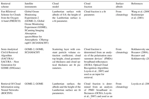
2 Should the surface albedo be a fit parameter? In this section, we discuss in some detail why in one of the two experimental conditions for the GOME-2A scene re-trievals we also fit the surface albedo when retrieving aerosol properties from the O2A band. It is difficult to separate ef-fects of the surface albedo and aerosol optical thickness from continuum reflectances, but independent information about the two parameters is available from the spectral shape of the absorption band: in the case of single scattering, photons backscattered by aerosols follow shorter paths through the atmosphere than photons reflected by the surface and they will thus have a smaller chance of being absorbed. Indeed, two different combinations of surface albedo and aerosol op-tical thickness that give the same continuum reflectance may be distinguished from their reflectance spectra inside the ab-sorption band, as is illustrated in Fig. 1 (left panel). The spec-trum plotted in red corresponds to the scenario of an aerosol layer between 700 and 600 hPa (Pmid of 650 hPa) with an optical thickness (τ) at 760 nm of 0.3 over a ground surface with albedo (As) of 0.2. The spectrum plotted in green cor-responds to the scenario of an aerosol layer with the same height and pressure thickness but with a different optical thickness and for a surface with a different albedo. The com-bination of aerosol optical thickness and surface albedo is chosen such that the continuum reflectance remains the same as in the first scenario. Note that the two spectra show differ-ences inside the absorption band. For comparison, the spec-trum plotted in blue corresponds to the scenario of an aerosol layer moved to a different height but with optical thickness and surface albedo kept the same as in the first scenario. This spectrum differs from the first two also inside the absorption band. Spectra are calculated for TROPOMI’s resolution in the near-infrared band of 0.38 nm (anticipated at the time of
writing). Also illustrated in Fig. 1 (right panel) are derivatives with respect to aerosol layer mid pressure (Pmid), aerosol optical thickness (τ) and surface albedo (As) for the exam-ple scenario. We cannot simultaneously fit surface albedo and aerosol optical thickness when the spectral shape of the derivatives is the same. The question of whether derivatives for a particular scenario are eventually sufficiently different has to be answered by actually doing the (non-linear) re-trieval and by subsequently performing an error analysis.
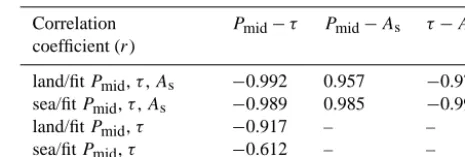
Of course, in order to simplify the retrieval problem one may ask whether it is possible to retrieve aerosol properties while fixing the surface albedo at values provided by cli-matologies. We have done retrieval simulations investigat-ing the effect on retrieved aerosol properties of uncertainties typically associated with surface albedo climatologies. Fig-ure 2 shows representative results for an aerosol layer over land (the example scenario mentioned above). We assume the climatological (a priori) 1σerror to be 0.02 for land sur-faces. The forward model and inversion scheme are the same as used in the GOME-2A retrievals (described in detail in Sect. 6), except for the instrument model (here TROPOMI spectral response function and noise model). Also, for sim-plicity we take the surface albedo to be independent of wave-length. The left panel shows biases in retrieved aerosol layer pressure when the true surface albedo deviates from the value assumed in retrieval (“climatology”). The three plot lines correspond to retrievals in which the surface albedo is not fitted (a priori error of 0.0), the surface albedo is fitted with an a priori error equal to the climatological error, and the surface albedo is fitted when unconstrained by a priori infor-mation (large a priori error of 0.2). When the surface albedo is fixed in the retrieval, small deviations of the true surface albedo cause pressure biases well above 100 hPa and non-convergent retrievals (missing data points). For darker sur-faces, the effect is more moderate but still significant. For example, when the true surface albedo is 0.04 but the albedo assumed in retrieval is 0.03, retrieved aerosol layer pressure for the example scenario is almost 100 hPa too high (not shown). The right panel of Fig. 2 illustrates the situation in a different way. In this plot we show precision of retrieved aerosol layer pressure and optical thickness as a function of the a priori error in the surface albedo. The three plot lines of the left panel thus correspond to three distinct points on the x axis of the plot in the right panel. One can see that auxil-iary information about the surface albedo should have a 1σ error smaller than about 10−3to 10−4 before it starts con-straining the retrieval of aerosol properties, which is a very small number. In other words, the O2 A band contains in-dependent information about the surface albedo and aerosol optical thickness. Of course, this information is more pro-nounced the more elevated aerosols are (i.e., the larger the pressure difference between the aerosols and the surface is).
Figure 1. Left panel: simulated top-of-atmosphere reflectance spectra for three different aerosol scenarios at a resolution of 0.38 nm. The
solar zenith angle is 50◦and the viewing direction is nadir. The spectrum plotted in red corresponds to the example scenario of an aerosol layer between 700 and 600 hPa with an optical thickness at 760 nm of 0.3 over a ground surface with albedo of 0.2. The spectrum plotted in green corresponds to the scenario of an aerosol layer with the same height and pressure thickness but with a different optical thickness and for a surface with a different albedo such that the continuum reflectance remains the same. For comparison, the spectrum plotted in blue corresponds to the scenario of an aerosol layer moved to a different height but with optical thickness and surface albedo the same as in the example scenario. Signal-to-noise ratios for these reflectance levels expected for TROPOMI are about 1000 in the continuum to about 250 in the deepest part of the absorption band. Right panel: derivatives of reflectance with respect to surface albedo, aerosol optical thickness and aerosol layer mid pressure for the example aerosol scenario. Derivatives are normalised to 1.0 at their respective maximums. Both panels: the aerosol has a single scattering albedo of 0.95 and a Henyey–Greenstein phase function with an asymmetry parameter of 0.7. The forward model for these calculations is the same as the forward model used in the GOME-2A retrievals. For simplicity, we assume the surface albedo to be independent of wavelength. Furthermore, the temperature profile corresponds to a mid-latitude summer atmosphere and the surface pressure is 1013 hPa.
Figure 2. Left panel: results of retrieval simulations showing the bias in retrieved aerosol layer mid pressure as a function of the true surface
albedo for three different a priori errors. The a priori value for the surface albedo is 0.20 (“climatology”). Results are shown for the example aerosol scenario (aerosol layer between 700 and 600 hPa with optical thickness at 760 nm of 0.3, surface albedo of 0.2). Missing data points indicate non-converging retrievals. Right panel: results of retrieval simulations showing precision of retrieved aerosol layer mid pressure and optical thickness as a function of the a priori error in the surface albedo. Both panels: a TROPOMI noise model is used which assumes shot noise throughout and a signal-to-noise ratio of 500 at 758 nm for a reference radiance of 4.5×10¹²photons s−1cm−2sr−1nm−1. The a priori error for aerosol layer mid pressure is 500 hPa and for aerosol optical thickness is 1.0. Other details are the same as in Fig. 1.
albedo climatologies. This is the first reason why we in-clude an experimental condition for the GOME-2A scene retrievals in which the surface albedo is fitted. The second reason to do so is explained in the following. Retrieval of aerosol pressure and optical thickness from the O2 A band requires of course an assumed aerosol model, but often ac-curate a priori information about the aerosol optical prop-erties is lacking. As discussed above, the target parameter of the TROPOMI O2 A band Aerosol Layer Height
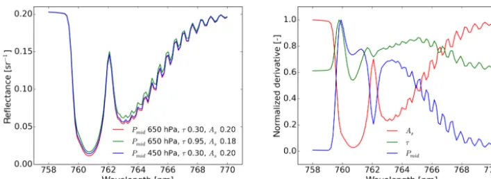
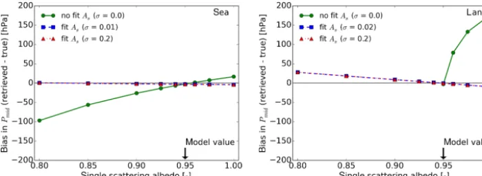
sur-face (right panel). One can see that in the case of a model error in the single scattering albedo, aerosol layer pressure is biased significantly and retrievals do not converge when the surface albedo is fixed in retrieval. Aerosol optical thick-ness and the surface albedo are biased as well (not shown). This effect is more moderate for the darker surface. For ex-ample, if the true single scattering albedo is 1.0 while the assumed value is 0.95, retrieved aerosol pressure is too high by about 20 hPa for aerosols over sea and by about 180 hPa for aerosols over land. Biases in retrieved aerosol layer pres-sures and non-convergences almost disappear when the sur-face albedo is included in the fit. Aerosol optical thickness and surface albedo, however, remain biased (not shown) and as a consequence retrieved values depend on the particular aerosol model assumed in retrieval (one might call them ef-fective quantities). Since aerosol height is the target param-eter, this finding is an important reason why at this stage of algorithm development we do not put effort in defining the most realistic aerosol model for every aerosol scene. Instead, in all retrievals presented in this paper we simply model the aerosol with a single scattering albedo of 0.95 and a Henyey– Greenstein phase function with asymmetry parameter of 0.7. As an important caveat, we mention that correlations be-tween errors in fit parameters for an O2A band aerosol re-trieval are typically very high. Absolute values of correlation coefficients (r) are often well above 0.9 and can sometimes become as high as 0.999. As an example, Table 2 lists corre-lation coefficients for retrieval of the example aerosol layer over land and over sea. The corresponding a posteriori er-rors, however, are small, as was shown in the right panel of Fig. 2. Apparently, parameters can be fitted with small pre-cision errors in the case that errors are indeed so highly cor-related. Derivatives of reflectance with respect to the various fit parameters are similar, yet there are small but significant differences (see right panel of Fig. 1), which cause correla-tion coefficients to be smaller than one and make it possi-ble to simultaneously fit parameters. Still, we should antici-pate retrieval becoming sensitive to the many other system-atic and quasi-random model and instrument errors present in real data when moving from the retrieval simulations re-ported in this section to the GOME-2A retrievals rere-ported in the next sections. Finally, we remark that we are not aware of previous studies on O2A band cloud or aerosol retrieval reporting a posteriori correlation coefficients.
3 Sensitivity of retrieved aerosol layer height and optical thickness to the aerosol optical properties As explained in the previous section, we apply a single aerosol model to the various GOME-2A scenes investigated in this study. From the perspective of operational processing, it is perhaps convenient to use a single aerosol model globally when the inaccuracy introduced in retrieved aerosol height is limited. But of course, we may optimise the assumed aerosol
Table 2. A posteriori correlation coefficients (r) for a simulated re-trieval of an aerosol layer between 700 and 600 hPa with optical thickness at 760 nm of 0.3 located over land and over sea. Either mid pressure and optical thickness or mid pressure, optical thick-ness and surface albedo are fitted. Other details are the same as in Figs. 1 and 2.
Correlation coefficient (r)
Pmid−τ Pmid−As τ−As
land/fitPmid,τ,As −0.992 0.957 −0.975 sea/fitPmid,τ,As −0.989 0.985 −0.999
land/fitPmid,τ −0.917 – –
sea/fitPmid,τ −0.612 – –
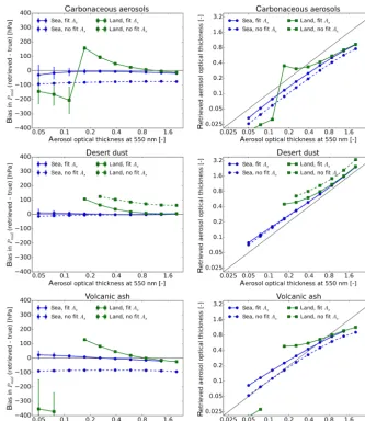
model or even implement a sophisticated model selection scheme at a later stage of algorithm development. We are not arguing against proceeding in that way here. In this sec-tion we discuss a more detailed sensitivity study investigat-ing the effect of errors in the assumed aerosol model on re-trieved aerosol layer height and aerosol optical thickness. We focus on desert dust, carbonaceous aerosols and volcanic ash, which are the dominant aerosol types in the free tropo-sphere. When they occur, these aerosols typically have rela-tively high optical thicknesses.
The desert dust model and the carbonaceous aerosol model are taken from the aerosol project of ESA’s Climate Change Initiative (CCI) program and they are described in De Leeuw et al. (2015). The coarse mode dust model is based onT -matrix calculations and the carbonaceous aerosol model is the fine mode strongly absorbing aerosol model based on Mie calculations. Finally, the volcanic ash model is based on the synthetic average volcanic aerosol model from the Amsterdam–Granada Light Scattering Database (Muñoz et al., 2012). The phase function for this model is the aver-age of measured phase functions for nine different volcanic ash samples (Muñoz et al., 2002, 2004; Volten et al., 2001). We calculated the extinction and scattering cross sections again from Mie theory using the average of the measured size distributions as reported by the Amsterdam–Granada database and a complex refractive index calculated from in situ measurements during the 2010 Eyja eruption as reported by Schumann et al. (2011; case “medium”). Extinction and scattering cross sections for the volcanic ash model are cal-culated at 630 nm, and we assume the same values at wave-lengths of the O2A band. Table 3 gives values for the extinc-tion cross secextinc-tion and single scattering albedo at 760 nm and other properties. Note that the carbonaceous aerosol and the volcanic ash have similar and relatively low single scattering albedos.
Figure 3. Results of retrieval simulations showing the bias in retrieved aerosol layer mid pressure as a function of the true single scattering
albedo for three different a priori errors in the surface albedo. The single scattering albedo assumed in retrieval is 0.95 (“model value”). The aerosol layer is over sea (albedo of 0.03, left panel) or over land (albedo of 0.2, right panel). Missing data points indicate non-converging retrievals. Other details are the same as in Figs. 1 and 2.
Table 3. Summary of aerosol models used in the sensitivity study of Sect. 3. The table lists the extinction cross section (Cext), single scattering albedo (ω) and asymmetry parameter (g) at 760 nm, and the ratio of the extinction cross section at 760 nm to the extinction cross section at the reference wavelength. The reference wavelength is 550 nm for the carbonaceous aerosol and desert dust model and 630 nm for the volcanic ash model.
Aerosol model Cext760 nm[µm−2] ω760 nm[–] g760 nm[–] Cext760 nm/Crefext[–]
Carbonaceous aerosol 1.8×10⁻² 0.76 0.57 0.57
Desert dust 1.1×10+1 0.97 0.71 1.0
Volcanic ash 1.6×10⁻¹ 0.76 0.65 1.0
Figure 4 shows the bias in retrieved aerosol layer mid pres-sure and retrieved aerosol optical thickness as a function of the true optical thickness. Biases in aerosol layer pres-sure are moderate for retrieval over sea. In the case of the dust aerosol, which absorbs only little in the near-infrared range, this is true even when the surface albedo is not fit-ted. For land, biases become larger or retrieval does not con-verge (missing data points). Fitting the surface albedo helps to ameliorate biases and improve convergence. These obser-vations confirm what has already been concluded in the pre-vious section. Furthermore, we see that for specific ranges of the optical thickness larger retrieval biases occur or biases become variable (see, for example, retrieval for the carbona-ceous aerosol between 0.1 and 0.2 optical thickness). The range in which retrieval becomes singular depends on the particular combination of aerosol optical thickness, aerosol height, aerosol optical properties (notably the phase func-tion), the surface albedo and the observation geometry and is therefore hard to predict. This has been noted before in Sanders and De Haan (2013). Such a singularity can also occur at higher aerosol optical thickness (see Sanders and De Haan, 2014). Comparing biases against the threshold re-quirement of 100 hPa, we see that biases are acceptable for optical thicknesses larger than about 0.2. With respect to non-converging retrievals, we remark that convergence can be im-proved by, for example, decreasing the signal-to-noise ratio, as we do in the GOME-2A retrievals presented below. The
measurement error covariance matrix in the retrieval simu-lations shown here is only filled with nominal noise errors, which may be too tight for convergence when also calibra-tion errors or other systematic errors are present.
We mention that more extensive retrieval simulations investigating the effects discussed above and many other retrieval sensitivities are presented in Sanders and De Haan (2014). In this paper, we present a number of sensi-tivity experiments using GOME-2A spectra, rather than sim-ulated spectra, to further investigate the retrieval. In conclu-sion, from simulation studies we learn that the surface albedo should be a fit parameter when retrieving aerosol properties from the O2 A band. In the following sections we investi-gate whether this conclusion also holds for retrievals with real spectra.
4 GOME-2 instrument characteristics
Figure 4. Results of retrieval simulations showing the bias in retrieved aerosol layer mid pressure (left column) and retrieved aerosol optical
thickness (right column) as a function of the true aerosol optical thickness for three different aerosol types (rows). Measurements are simu-lated for a carbonaceous aerosol (top row), a desert dust (middle row) and a volcanic ash type (bottom row), while in the retrieval the default aerosol model is assumed (single scattering albedo of 0.95 and a Henyey–Greenstein phase function with asymmetry parameter of 0.7). The four plot lines correspond to sea (blue, circles) and land (green, squares) and to not fitting (dashed lines) and fitting (solid lines) the surface albedo. The aerosol layer is located between 700 and 600 hPa. Missing data points indicate non-converging retrievals. The solar zenith angle is 50◦and the viewing direction is nadir. All other settings are the same as in the simulation study of Sect. 2 (see also Figs. 1 and 2).
only forward pixels are considered. The scan speed profile is such that the across track pixel size is approximately con-stant. The across track pixel size is mainly determined by the integration time, which generally is 0.1875 s for spectrometer Band 4 for the sunlit part of the orbit track. Thus, the across track forward pixel size is 80 km for the nominal 1920 km swath and 40 km in reduced swath mode (aerosol scene 06 in this work). The along track pixel size at nadir is 40 km and is primarily determined by the instrument’s along track in-stantaneous field of view. Band 4 runs from 584 to 798 nm and has a spectral sampling of about 0.21 nm. The instru-ment spectral response function in Band 4 has a full width at half maximum (FWHM) of approximately 0.53 nm, which
5 Selection of aerosol scenes and masking of clouds
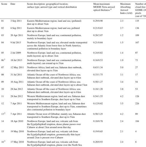
We first compiled a list of 16 aerosol scenes that served as an input for the GOME-2A retrieval experiments. In this paper, we define a scene as a 3-minute granule of GOME-2A observations, which covers an area of about 1920 km across track by 1200 km along track (at nadir) for ground pixel sizes of 80 by 40 km (at nadir). Scenes were se-lected not only for the presence of aerosols but also for the availability of lidar measurements within the scene. We initially focussed on ground-based measurements because we might find good spatiotemporal collocation with the GOME-2A overpass for these lidar measurements. Ground-based measurements from the Cabauw Experimental Site for Atmospheric Research (CESAR) and the EARLINET sta-tion at Cabauw (Netherlands), from EARLINET stasta-tions at Evora (Portugal) and Granada (Spain), and from the Micro Pulse Lidar NETwork (MPLNET) station at Santa Cruz (Ca-nary Islands) are included in this study. We also used airborne measurements taken aboard the Facility for Airborne At-mospheric Measurements’s (FAAM) AtAt-mospheric Research Aircraft during two dedicated campaigns over the North Sea (Eyjafjallajökull eruption) and the Aegean Sea (the Eu-ropean Space Agency’s CARBONEXP campaign). Finally, we took satellite-based lidar measurements from CALIPSO into account. The initial checking of the presence of signif-icant amounts of aerosols and of cloud conditions was done using AERONET aerosol optical thickness plots, lidar quick-looks and RGB images from the MODerate resolution Imag-ing Spectroradiometer (MODIS). Table 4 provides a short description of the 16 aerosol scenes that were eventually se-lected.
Having lidar measurements available within the geograph-ical area of the aerosol scene that are also reasonably close in time to the GOME-2A overpass is a severe constraint, be-cause of the sparse spatiotemporal sampling of lidar mea-surements. For example, exceptionally thick ash plumes close to an erupting volcano, which may have been an easy starting point for our case studies, were not included as there are no such aerosol cases (to our knowledge) for which there are nearby lidar measurements. As a consequence, the aerosol scenes have aerosol optical thicknesses that are mod-erate (see Table 4).
GOME-2A aerosol scenes were cloud-cleared using four conventional AVHRR threshold tests (EUMETSAT, 2011). These tests are (i) a brightness temperature test in the 11 µm channel to detect medium to high clouds, (ii) a brightness temperature difference test for the 11 and 12 µm channels to detect thin cirrus clouds, (iii) an albedo test using the two vi-sual channels (one for land, the other for sea) to detect bright low clouds, and (iv) a spatial coherence test for the 11 µm channel to detect broken clouds over sea. For every AVHRR pixel, if one of the tests indicated the presence of a cloud, the AVHRR pixel was considered cloudy. Then, a cloud frac-tion for the GOME-2A ground pixel was derived by dividing
the number of cloudy AVHRR pixels by the total number of AVHRR pixels falling within the spectrometer’s footprint. Aerosol height retrievals in this paper are only attempted for GOME-2A pixels with zero AVHRR cloud fraction. Table 4 lists the number of cloud-free pixels for every aerosol scene. We mention here that we did not take AVHRR cloud infor-mation directly from the AVHRR level-1b product but used EUMETSAT’s (European Organisation for the Exploitation of Meteorological Satellites) new Polar Multi-sensor Aerosol Properties product (PMAp) instead (EUMETSAT, 2014b). This product provides spectral aerosol optical thickness de-rived from GOME-2’s PMD broadband radiances. As a sup-port field, PMAp also provides an AVHRR cloud fraction for PMD ground pixels using the approach described above. AVHRR pixels are accurately collocated to PMD ground pix-els (EUMETSAT, 2014b). We used cloud fractions for PMD ground pixels to calculate cloud fractions for spectrometer ground pixels.
Table 4. Description of the 16 aerosol scenes used in the GOME-2A retrieval experiments. Here, an aerosol scene is a 3-minute granule of
GOME-2A observations, which consists of 720 pixels in total.
Scene Date Scene description: geographical location; surface type; aerosol type and vertical distribution
Mean/maximum MODIS Terra aerosol optical thickness4
Maximum Absorbing Aerosol Index (AAI)
Number of cloud-free GOME-2A pixels (out of 720)5
01 3 Sep 2011 Eastern Mediterranean region; land and sea; (polluted) dust up to about 5 km
0.29/0.90 2.3 135
02 6 Sep 2011 Eastern Mediterranean region; land and sea; polluted dust up to about 3 km
0.21/0.63 2.7 136
03 20 Apr 2011 Northwest Europe; land and sea; continental pollution, mainly in boundary layer
0.28/2.07 1.2 109
04 9 Jul 2013 Northwest Europe; land and sea; elevated smoke transported across the Atlantic from forest fires in North America, continental pollution in boundary layer
0.21/0.64 1.5 167
05 2 Jul 2009 Northwest Europe; land and sea; continental pollution, multi-layered, up to about 2 km
0.24/0.82 1.4 87
061 18 Jul 2013 Northwest Europe; land and sea; continental pollution, multi-layered, can extend up to 5 km
0.16/0.53 1.0 73
07 12 May 2011 Northwest Africa; land and sea; Saharan dust outbreak, elevated dust layers up to 5 km
0.63/1.34 5.0 27
08 31 Jul 2011 Atlantic Ocean off the coast of Northwest Africa; sea; Saharan dust outbreak, elevated dust layers up to 6 km
0.33/1.75 3.1 17
09 10 Aug 2011 Atlantic Ocean off the coast of Northwest Africa; sea; Saharan dust outbreak, elevated dust layers up to about 5 km
0.58/1.27 3.4 54
10 28 Jun 2012 Atlantic Ocean off the coast of Northwest Africa; sea; Saharan dust outbreak, elevated dust layers up to 6 km
0.18/1.20 3.8 53
11 28 Jun 2012 Western Mediterranean region; land and sea; Saharan dust transported to Southern Europe, dust layer up to 5 km
0.54/1.55 4.2 126
12 7 Apr 2011 Western Mediterranean region; land and sea; Saharan dust transported to Southern Europe, dust up to 5 km, sometimes also continental pollution in boundary layer
0.12/0.82 3.5 226
132 7 Apr 2011 Atlantic Ocean west of Gibraltar; mainly sea; Saharan dust transported to Southern Europe, dust up to 5 km
0.58/3.25 4.2 89
14 18 Apr 2010 Northwest Europe; land and sea; volcanic ash from the Eyjafjallajökull eruption, dense plume passes over Cabauw at about 2 km around noon that day
0.18/0.78 2.4 184
15 19 May 2010 Northwest Europe; land and sea; volcanic ash from the Eyjafjallajökull eruption, geometrically thin layer around 2 km is present over Cabauw
0.19/0.65 2.1 4
163 17 May 2010 Northwest Europe; land and sea; volcanic ash from the Eyjafjallajökull eruption, plume over the North Sea between about 4 and 6 km
0.28/0.93 2.4 6
1Reduced swath for GOME-2 on Metop-A: ground pixels are 40 km by 40 km. 2This dust outbreak is described in detail in Preißler et al. (2011).
3The flight of the FAAM aircraft and measurements taken aboard are described in Johnson et al. (2012).
4Mean and maximum of MODIS Terra aerosol optical thicknesses (at 550 nm) for MODIS ground pixels collocated with GOME-2A pixels in the scene. MODIS aerosol optical thicknesses are
from Dark Target Land and Ocean algorithms. Note that the Terra platform lags Metop-A by about 1 hour.
5For a description of the cloud mask applied to the GOME-2A spectrometer pixels, see main text.
do a first comparison. A validation is beyond the scope of this paper, and given the present GOME-2A retrieval results it is not needed for our purposes at this point (to be discussed in detail in Sect. 9). We will primarily use lidar measurements to better understand the difference in retrieval outcome when
Table 5. Description of the lidar measurements that are used in the comparison with retrieved aerosol heights for GOME-2A target pixels.
Spatial distance is the distance between the centre of the GOME-2A target pixel and the location of the lidar measurement. Recall that GOME-2A pixels are usually 80 km by 40 km. Temporal distance is defined as the time of the lidar measurement minus the observation time for the GOME-2A target pixel. Reported lidar extinction profiles are not instantaneous but averaged over a certain time window. Averaging times vary with lidar systems and atmospheric conditions.
Scene Lidar description Spatial distance
to target pixel [km]
Temporal distance to target pixel [hh:mm]
Remarks
01 FAAM aircraft; extinction at 355 nm 81 km +01:14 Assumed lidar ratio 65 sr
02 CALIPSO; extinction at 532 nm 102 km about+02:35 CALIPSO level-2
03 Cabauw/CESAR; extinction at 355 nm 46 km 00:00 Assumed lidar ratio 50 sr
04 Cabauw/EARLINET; extinction at 355 nm
148 km about+01:45 Raman lidar measurement
CALIPSO; extinction 532 nm 140 km about+02:43 CALIPSO level-2
05 CALIPSO; extinction 532 nm 14 km about+02:50 CALIPSO level-2
Cabauw/EARLINET; extinction at 355 nm
429 km about−01:37 Raman lidar measurement
06 CALIPSO; extinction 532 nm 55 km about+02:24 CALIPSO level-2
Cabauw/EARLINET; extinction at 355 nm
504 km +01:31 Assumed lidar ratio 50 sr
07 CALIPSO; extinction 532 nm 43 km about+03:27 CALIPSO level-2
Santa Cruz/MPLNET; extinction at 532 nm
540 km about−00:15 Assumed lidar ratio 50 sr
08 Santa Cruz/MPLNET; extinction at 532 nm
244 km about−02:02 Assumed lidar ratio 50 sr
09 Santa Cruz/MPLNET; extinction at 532 nm
106 km about+00:06 Assumed lidar ratio 50 sr
10 CALIPSO; extinction 532 nm 8 km about+03:34 CALIPSO level-2
Santa Cruz/MPLNET; extinction at 532 nm
1143 km about+00:16 Assumed lidar ratio 50 sr
11 CALIPSO; extinction 532 nm 145 km about+03:42 CALIPSO level-2
Granada/EARLINET; extinction at 355 nm
47 km about+10:00 Raman lidar measurement
12 Granada/EARLINET; extinction at 532 nm
101 km +00:02 Assumed lidar ratio 50 sr
13 Evora/EARLINET; extinction at 355 nm
4 km about−07:07 Raman lidar measurement
CALIPSO; extinction 532 nm 142 km about+02:36 CALIPSO level-2
14 Cabauw/CESAR; extinction at 355 nm
76 km +00:01 Assumed lidar ratio 50 sr
15 Cabauw/CESAR; extinction at 355 nm
168 km +01:39 Assumed lidar ratio 50 sr
16 FAAM aircraft/extinction at 355 nm 318 km +04:54 Assumed lidar ratio 65 sr
6 Description of the retrieval setup
Here, we summarize main aspects of the forward model and the inversion scheme and describe the implementation for retrievals with GOME-2A as presented in this paper.
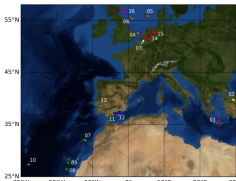
Figure 5. Overview of GOME-2A target pixels (numbered
quad-rangles) and corresponding lidar measurements (circles). The dar measurements are described in Table 5. Color code for li-dar measurements: FAAM aircraft (magenta), CALIPSO (yel-low), Cabauw (red), Santa Cruz (green), Granada (blue), and Evora (cyan). For some pixels, two lidar measurements are avail-able for evaluation. There are nine GOME-2A target pixels over sea (target pixels 01, 04, 05, 06, 07, 08, 09, 10, 16) and seven over land (target pixels 02, 03, 11, 12, 13, 14, 15). The aerosol scenes are described in Table 4.
6.1 Forward model
Monochromatic reflectances in the O2 A band are calcu-lated online using the doubling-adding method (e.g., De Haan et al., 1987; Hovenier et al., 2004). Multiple scat-tering is included in the calculations, but polarisation and rotational Raman scattering are ignored. An efficient high-resolution wavelength grid is constructed by defining small wavelength intervals bounded by strong O2 line positions and using Gaussian division points for each interval. This results in about 3000 line-by-line calculations for a fit win-dow extending from 758 to 770 nm and an oxygen absorp-tion cross secabsorp-tion that includes the three major isotopo-logues. The atmosphere is divided into 24 homogeneous lay-ers, the distribution of which is not equidistant but again follows a Gaussian integration scheme. Finally, 9 Gaussian points (18 streams) are used for integration over the polar angle. Derivatives are calculated in a semi-analytical man-ner using reciprocity (equivalent to the adjoint method, e.g., Landgraf et al., 2001).
In addition to line absorption by O2, first-order line mix-ing and collision-induced absorption by O2-O2 and O2-N2 are included in the oxygen absorption cross section accord-ing to Tran et al. (2006) and Tran and Hartmann (2008). Line parameters for the three major isotopologues are taken from the Jet Propulsion Laboratory database in agreement with Tran and Hartmann (2008). In the baseline retrieval setup,
the resulting absorption cross section is multiplied by 1.03 following Butz et al. (2013) and Crisp et al. (2012).
Temperature profiles and surface pressures were taken from the European Centre for Medium-range Weather Fore-casts’ (ECMWF) Interim reanalysis fields. Reanalysis data are available every 6 h (model times: 00:00, 06:00, 12:00, and 18:00 UTC) with a native spatial resolution of about 80 km. We used data on a 0.5◦ by 0.5◦ regular latitude–longitude grid. Note that this resolution is comparable to the size of the GOME-2 pixel. In the spatial dimension we took meteoro-logical data for the model grid point closest to the center co-ordinate of the GOME-2A pixel. In the temporal dimension, we used linear interpolation between the two closest model times to determine meteorological parameters at the time of the GOME-2A observation.
Next to oxygen absorption and Rayleigh scattering, scat-tering and absorption by aerosols takes place in the atmo-sphere. In the baseline retrieval setup, we assume a single aerosol layer that is modelled as a layer of particles with a constant particle volume extinction coefficient and parti-cle single scattering albedo. Also the pressure thickness is assumed constant and taken to be 50 hPa in all GOME-2A re-trievals. By default, aerosols have a single scattering albedo of 0.95 and a Henyey–Greenstein phase function with asym-metry parameter of 0.7. There is no particular reason for choosing these values of single scattering albedo and asym-metry parameter other than that they are intermediate to val-ues typically observed (Dubovik et al., 2002). In a similar fashion, we choose a phase function that is smooth and can serve as an approximate phase function for many aerosol types.
The ground surface is modelled as a Lambertian surface, and we allow the surface albedo to depend linearly on wave-length. Albedo values at two wavelength nodes located at the end points of the fit window (758 and 770 nm) are speci-fied and intermediate values are determined by interpolation. A priori values for the albedo at the two nodes are taken from the MERIS black-sky albedo climatology (Popp et al., 2011). Note that for sea pixels this climatology is filled with val-ues from the GOME Lambertian-equivalent reflectivity cli-matology (Koelemeijer et al., 2003). In one of the sensitiv-ity experiments of Sect. 8, we investigate the effect of fitting fluorescence emissions. Chlorophyll fluorescence from ter-restrial vegetation is modeled as an isotropic contribution to the upwelling radiance field at the surface. Also fluorescence emissions are allowed to depend linearly on wavelength and they are specified at the same two wavelength nodes as the surface albedo. We assume fluorescence emissions to be ab-sent a priori.
smooth (i.e., low-order polynomial in wavelength) additive offset to the simulated measured radiance spectrum. In one of the sensitivity experiments of Sect. 8, we include a spectrally constant stray light offset in the fit and assume the offset to be absent a priori. We specify the additive radiance offset as a percentage of the continuum radiance at 758 nm.
6.2 Inversion
GOME-2A level-1b files provide radiance spectra and a daily irradiance measurement. The product also provides a noise spectrum for each radiance measurement, which we call the nominal noise in this paper. Level-1b files from the latest pro-cessor version 5.3 are used.
The atmospheric state vector is determined through a spec-tral fit of reflectance across the fit window running from 758 to 770 nm and using the Optimal Estimation frame-work (Rodgers, 2000). The state vector contains in any case aerosol layer mid pressure (Pmid) and aerosol optical thick-ness (τ) at 760 nm. Depending on the experimental condi-tion, the state vector may contain other parameters as well. State vector elements, a priori values and a priori errors are summarised in Table 6. A positive temperature offset means that the entire a priori ECMWF temperature profile is shifted by the offset amount to higher temperatures in the retrieval.
Gauss–Newton iteration is used to find a minimum in the cost function, which is an efficient method if the forward model is only moderately non-linear. However, in the case of non-linear behaviour of the forward model, convergence and the retrieval solution itself may depend on the starting values for the iteration. For example, it has been noted in simulation experiments that the cost function for O2A band aerosol re-trieval may have multiple local minima (e.g., Fig. 19 in Holl-stein et al., 2012; Fig. 6-1 in Sanders and De Haan, 2014). One of the aims of the retrieval experiments reported in this paper is therefore to systematically investigate convergence and stability of the retrieval. For that reason, we now discuss in somewhat more detail the implementation of the Gauss– Newton method in our retrieval setup.
Gauss–Newton iteration is embedded in an iterative scheme with two modifications. First, when the initial state differs strongly from the true state, it is known that the update of the state vector in the case of Gauss–Newton iteration can become very large and lead to a point in state space far from the correct solution. Therefore, if the update of the state vec-tor becomes larger than a pre-defined threshold, we reduce the size of the update. We do this by temporarily decreas-ing the signal-to-noise ratio of the measurement until the update falls below the threshold. In our GOME-2A retrieval experiments, reduction of the state vector update occurs al-most every run, particularly during the first few updates. Sec-ond, parameters can attain non-physical values during itera-tion (e.g., negative optical thickness). For various parameters we have therefore defined boundaries. If a state vector ele-ment crosses such a boundary, we simply reset the eleele-ment
to that boundary value. We prefer this method to transfor-mations that make such boundary crossings impossible (e.g., fitting of the logarithm of the optical thickness) because we have experienced that such transformations tend to make the model more non-linear. In our GOME-2A retrieval experi-ments, we see that boundary resets occur regularly during it-eration, also for retrievals that subsequently converge. Exam-ples of boundaries are 0.01 for the minimum aerosol optical thickness and 15 km for the maximum altitude of the aerosol layer.
The maximum allowed number of iterations is 12. Based on results from the GOME-2A retrieval experiments (to be discussed below), we do not expect convergence to signifi-cantly improve if this number is increased. An initial round of experiments suggested that convergence does improve sig-nificantly if the nominal noise as given in the level-1b prod-uct is increased. In these preliminary experiments, we found that multiplying the nominal noise by two improves conver-gences but does not introduce new retrieval solutions. In all GOME-2A retrieval experiments reported in this paper (the scene retrievals of Sect. 7 as well as the sensitivity experi-ments of Sect. 8), the nominal noise has therefore first been multiplied by two before a retrieval is attempted.
Finally, convergence and stability of the retrieval is tested by always running the retrieval for a particular GOME-2A pixel in a particular experimental condition multiple times with different initial values. Typically, retrieval is attempted for three initial values for the aerosol layer mid pressure and two initial values for the optical thickness (six runs in total).
7 Results of GOME-2A scene retrievals
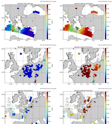
Figure 6 shows retrieved aerosol layer mid pressure and aerosol optical thickness for three representative scenes when the surface albedo is not fitted and Fig. 7 shows results for the same scenes when the surface albedo is included in the fit. In both cases also a temperature offset is retrieved. Re-trieval is only attempted for cloud-free pixels according to the AVHRR cloud mask described above. Retrievals that did not converge for any of the six attempted runs (i.e., for any of the six different sets of initial values) are represented in white; for retrievals that had at least one convergent run, the solution with the smallestχ2-value is shown. Quadrangles with red borders indicate pixels that are inside the sun glint region (i.e., sun glint angle smaller than 18◦). These pixels are included in the scene retrievals. For every scene, the tar-get pixel, which is used in more extensive sensitivity exper-iments (Sect. 8) and for which retrieved aerosol layer height is compared against lidar profiles, is indicated with a thick black border. Note that target pixels are always selected out-side the sun glint region. Finally, spatial locations of the lidar measurements are indicated with a purple dot.
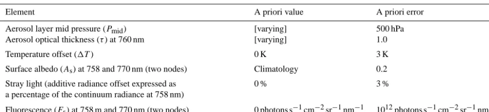
Table 6. State vector elements, a priori values and a priori (1σ) errors. In the default retrieval setup for the GOME-2A scene re-trievals (Sect. 7), only the first three or five parameters are fitted. Retrieval is attempted multiple times with different initial values for aerosol layer mid pressure and aerosol optical thickness. Fitting stray light or fluorescence emissions is only done in sensitivity experiments reported in Sect. 8.
Element A priori value A priori error
Aerosol layer mid pressure (Pmid) [varying] 500 hPa
Aerosol optical thickness (τ) at 760 nm [varying] 1.0
Temperature offset (1T) 0 K 3 K
Surface albedo (As) at 758 and 770 nm (two nodes) Climatology 0.2
Stray light (additive radiance offset expressed as a percentage of the continuum radiance at 758 nm)
0 % 3 %
Fluorescence (Fs) at 758 m and 770 nm (two nodes) 0 photons s−1cm−2sr−1nm−1 1012photons s−1cm−2sr−1nm−1
fitted and 1401 pixels had at least one converging run when the surface albedo was fitted. Including the surface albedo in the state vector raised the average number of iterations needed for convergence from 3.9 to 6.5. The average calcula-tion time for one iteracalcula-tion (spectrum and derivatives) is about 30 s on an up-to-date desktop computer. We remark that the computer code is a non-optimised science code.
In agreement with our expectation from the simulation study of Sect. 2, we see poorer convergence when the sur-face albedo is not fitted. This would then be due to, for ex-ample, the model value from the surface albedo climatology being inaccurate. Also inaccuracies in the assumed aerosol model could play a role here. Interestingly, a significant num-ber of pixels still show converging retrievals when the surface albedo is fixed in retrieval. When the surface albedo is fitted, most pixels had at least one converging run. However, in that case we find that retrieved pressures are systematically and significantly lower (i.e., aerosol layer higher in atmosphere), which is unexpected. The systematic differences in retrieved aerosol layer pressure between the two experimental condi-tions are typically larger than the biases found in the sim-ulation study of Sect. 2. This suggests that other, stronger effects are interfering in the GOME-2A retrievals. Also note that retrieved aerosol layer mid pressures show more realis-tic values when not fitting the surface albedo than when fit-ting. Finally, we remark that retrieved parameter values often show an east–west gradient, or rather an interaction with the viewing zenith angle, as well as a land–sea interaction. These interactions could be related to, for example, model errors in the phase function. Such a model error affects retrieved op-tical thickness and, because of correlated errors, also aerosol pressure.
Figure 8 shows PMAp aerosol optical thickness at 550 nm against retrieved aerosol optical thickness (at 760 nm) for both experimental conditions. PMAp retrieves spectral aerosol optical thickness for PMD ground pixels. The the-oretical basis is described in EUMETSAT (2014b) and a first validation with AERONET aerosol optical thickness is re-ported in EUMETSAT (2014c). Eight PMD ground pixels
make up one spectrometer ground pixel. In Fig. 8, the mean of valid PMD subpixel PMAp aerosol optical thicknesses is compared against the aerosol optical thickness retrieved from the O2A band. Thus, PMAp aerosol optical thickness is spatiotemporally collocated with the spectrometer measure-ments that we use for our O2A band retrievals. Note that at the time of writing, PMAp aerosol optical thickness was only available for sea pixels. We have also compared retrieved aerosol optical thickness with MODIS Terra aerosol optical thickness, which is available for land surfaces as well, but the correlation was worse. This is probably due to the different overpass times of the Metop-A and Terra satellites.
It is important to remark that an absolute validation of retrieved aerosol optical thickness is neither attempted here nor expected, because PMAp aerosol optical thickness is re-ported at a different wavelength and our optical thickness is an effective quantity, which holds for the aerosol model assumed in the retrieval (see Sect. 2). However, if our O2 A band retrieval is indeed picking up an aerosol signal, we do expect a significantly positive correlation with PMAp aerosol optical thickness when many different aerosol scenes are in-cluded in the comparison. PMAp aerosol optical thickness correlates significantly with retrieved O2A band aerosol op-tical thickness when not fitting the surface albedo (left panel of Fig. 8). When fitting the surface albedo, the situation be-comes less clear. The data appear to separate into two clus-ters (which is the reason why a linear regression is not per-formed) and retrieved O2A band aerosol optical thickness for the denser one is significantly lower than PMAp aerosol optical thickness. We come back this observation in Sect. 11.
con-Figure 6. Retrieved aerosol layer mid pressure (left column) and aerosol optical thickness (right column) for three representative GOME-2A
scenes (rows) when the surface albedo is fixed in retrieval. The depicted aerosol scenes are (from top to bottom) scene 01, scene 03, and scene 04 from Table 4. Next toPmidandτ(760 nm), a temperature offset1T is fitted. The layer’s assumed pressure thickness is 50 hPa. The model value for the surface albedo is taken from the MERIS black-sky albedo climatology (Popp et al., 2011). Pixels that had no converging retrieval for any of the six attempted runs (i.e., for any of the different sets of initial values) are plotted in white. Missing pixels are pixels that did not pass cloud filtering. The target pixel that is used in the sensitivity experiments of Sect. 8 is depicted with a thick black border. Quadrangles with red borders indicate pixels that are inside the sun glint region. Finally, spatial locations of the lidar measurements are shown with purple dots. Values outside the ranges depicted are clipped.
vergence and the retrieval solution of the assumed aerosol model, scaling of the oxygen absorption cross section and fitting of a temperature offset, fitting of the surface albedo, and fitting of a stray light offset or a fluorescence emission.
In the first experiment we investigate the effect of the assumed aerosol model. The retrieval setup is the same as in Sect. 7 and the surface albedo is fixed in retrieval (as in Fig. 6) or it is retrieved (as in Fig. 7). Figure 8 shows the fraction of converged runs, retrieved aerosol layer mid pressure, aerosol optical thickness and surface albedo (only
Figure 7. Retrieved aerosol layer mid pressure (left column) and aerosol optical thickness (right column) for the same GOME-2A
scenes (rows) as in Fig. 6 when including the surface albedo in the state vector. Next to Pmid andτ (760 nm), the surface albedoAs and a temperature offset1T are fitted. Other settings are the same as in Fig. 6.
particle with single scattering albedo at 760 nm of 0.97 and a phase function with asymmetry parameter of 0.58. The lat-ter model is the fine mode weakly absorbing aerosol type from the aerosol-CCI project (see De Leeuw et al., 2015). These aerosol models are chosen for no other reason than that they show some variability in microphysical properties. In this experiment and in all other sensitivity experiments de-scribed in Sect. 8, retrieval is attempted for four initial values of the aerosol layer mid pressure and three initial values of the optical thickness (12 runs in total). The fraction of con-verged runs is thus defined as the number of concon-verged runs divided by 12. Finally, retrieved parameter values for the so-lution with the smallestχ2-value are shown and whiskers in-dicate the maximum to minimum range of retrieval solutions.
In the first place, this experiment confirms the observation made before in the simulation study of Sect. 2 that the as-sumed aerosol model has only a moderate effect on retrieved aerosol pressure. Interestingly, when the same experiment is repeated but without fitting the surface albedo, we see that the effect of the assumed aerosol model remains quite mod-erate for many pixels (although a number of other pixels now fail to have converging runs). In the second place, we see that retrieval is very stable. Most of the 12 runs (i.e., retrieval at-tempts for different sets of initial values) converge and they usually converge to the same retrieval solution.
Figure 8. PMAp aerosol optical thickness at 550 nm against aerosol optical thickness retrieved from the O2A band measured with GOME-2A when the surface albedo is not fitted (left panel) and when it is (right panel). In these plots, PMAp aerosol optical thickness is the mean of valid PMAp retrievals (at least one) for PMD subpixels within the GOME-2A spectrometer’s footprint.
Figure 9. Fraction of converged runs (top left), retrieved aerosol layer mid pressure (top right), retrieved aerosol optical thickness (bottom
Figure 10. Retrieved aerosol layer mid pressure (left) and aerosol optical thickness (right) for 16 GOME-2A target pixels and three different
aerosol models. Details are the same as in Fig. 9, except that now the surface albedo is fixed in retrieval (as in Fig. 6).
baseline retrieval setup of Sect. 7. The left panel shows rel-ative residuals when the surface albedo is fixed in retrieval and the right panel when the surface albedo is fitted. Relative residuals are defined as (Rmeas−Rfit)/Rmeas·100 %. It is clear that residuals have a distinct spectral structure, which can be a starting point for future investigations. We have residuals up to about 24 % when the surface albedo is not fit-ted and residuals up to about 8 % when the surface albedo is retrieved. It should be noted, however, that relative residuals peak inside the absorption band where reflectances can be up to a factor of 10 smaller than in the continuum. In particular, the difference between the two conditions is mainly a peak in the R-branch around 760.5 nm, but otherwise, relative resid-uals are very similar in magnitude. Absolute fit residresid-uals are indeed spectrally more flat. Figure 12 shows the measured and modeled reflectance spectra and the absolute residuals for two example pixels. From these plots the difference be-tween fitting and not fitting the surface albedo is less pro-nounced. Interestingly, absolute residuals when not fitting the surface albedo appear to have a slope, which is perhaps re-lated to an incorrect wavelength dependence of the surface albedo as this dependence is basically determined by the sur-face albedo climatology.
In the second experiment we investigate the effect of scal-ing the oxygen absorption cross section and fittscal-ing of a tem-perature offset. Recall that in the default retrieval setup, the calculated oxygen absorption cross section is increased by 3 % in agreement with Butz et al. (2013) and Crisp et al. (2012), and an offset to the a priori ECMWF temper-ature profile is fitted. Figure 13 shows the fraction of con-verged runs and retrieved aerosol layer mid pressure for three experimental conditions. In the first condition, neither the oxygen absorption cross section is scaled nor a temperature offset is fitted. In the second condition, the oxygen absorp-tion cross secabsorp-tion is increased by 3 %. In the third condiabsorp-tion, also a temperature offset is fitted. This latter condition then corresponds to the default retrieval setup.
We observe that convergence for the set of target pixels improves when the oxygen absorption cross section is scaled and when a temperature offset is fitted. In fact, for two tar-get pixels none of the 12 runs converges in the base condi-tion, while all 12 runs converge when the absorption cross section is scaled and a temperature offset is fitted. The sig-nificant improvement of convergence is the reason why we did both in the default retrieval setup for the scene retrievals. There are small but systematic effects on retrieved parameter values; this is generally expected, considering the high cor-relations between errors in fit parameters discussed above. Furthermore, we find that retrieved temperature offsets are always negative and ranging from about −4 to −8 K (not shown). This means that for every GOME-2A pixel the en-tire a priori temperature profile, which we constructed from ECMWF reanalysis data at high spatial resolution, is shifted to lower temperatures by this amount in the retrieval. Ap-parently, fitting a temperature offset compensates for model errors other than remaining inaccuracies in meteorological data, as the temperature offset would have been random and much smaller in magnitude in that case. (Note that we are re-trieving aerosol in cloud-free, hence meteorologically stable, conditions.) Finally, we remark that, although convergence improves, retrievals that converged in all three conditions do not show an overall and systematic decrease in spectral fit residuals. Some peaks slightly decrease but other peaks slightly increase.
Figure 11. Fit residuals for all converged runs for the 16 GOME-2A target pixels. The default retrieval setup of Sect. 7 is used. Left panel:
surface albedo not fitted (see Fig. 6); right panel: surface albedo fitted (see Fig. 7). Relative residues are defined as (Rmeas−Rfit)/Rmeas· 100 %.
Figure 12. Measured and modeled reflectance spectra for two example GOME-2A target pixels. Top row: pixel over sea (target pixel 04);
bottom row: pixel over land (target pixel 13). Left column: surface albedo not fitted; right column: surface albedo fitted. Absolute residues are defined asRmeas−Rfit. The default retrieval setup of Sect. 7 is used and the run with the smallestχ2-value is shown.
emission is typically spectrally smooth and here allowed to depend linearly on wavelength across our fit window.
When fitting the surface albedo, including a stray light off-set in the state vector does not show a systematic improve-ment of the retrieval. The fraction of converged runs stays the same or perhaps slightly decreases. At the same time we do not observe a systematic decrease of fit residuals. Inter-estingly, we find that the retrieved radiance offset is typically quite large and negative (ranging from 0 to−5 % and on av-erage −2.5 % of the continuum radiance). A negative off-set means that light is removed from the spectrum. At the