On the shelf resonances of the Gulf of Carpentaria and the Arafura Sea

(1)

doi:10.5194/os-8-733-2012

On the shelf resonances of the Gulf of Carpentaria and

the Arafura Sea

D. J. Webb

National Oceanography Centre, Southampton SO14 3ZH, UK Correspondence to: D. J. Webb (djw@soton.ac.uk)

Received: 20 December 2011 – Published in Ocean Sci. Discuss.: 3 February 2012 Revised: 29 June 2012 – Accepted: 6 July 2012 – Published: 1 September 2012

Abstract. A numerical model is used to investigate the res-onances of the Gulf of Carpentaria and the Arafura Sea, and the additional insights that come from extending the analysis into the complex angular velocity plane. When the model is forced at the shelf edge with physically realistic real values of the angular velocity, the response functions at points within the region show maxima and other behaviour which imply that resonances are involved but provide little additional in-formation. The study is then extended to complex angular velocities, and the results then show a clear pattern of grav-ity wave and Rossby wave like resonances. The properties of the resonances are investigated and used to reinterpret the response at real values of angular velocity. It is found that in some regions the response is dominated by modes trapped between the shelf edge and the coast or between opposing coastlines. In other regions the resonances show cooperative behaviour, possibly indicating the importance of other phys-ical processes.

1 Introduction

Observational studies of the tides and the success of the stan-dard method of tidal prediction show that although non-linear effects are present, the response of the ocean to tidal forc-ing is predominantly linear. In terms of understandforc-ing ocean physics, this is important because it means that we can make use of the theory of linear operators. Such an approach has been very successful in the development of many other areas of physics.

One of the theory’s main results is that the response of lin-ear systems can be expressed in terms of a Green’s function (Webb, 1973b), and that this is an analytic function of

an-gular velocity with poles at the eigenvalues or resonances of the system. The response to a particular forcing, the response function, has similar properties. The residue at its poles has a spacial structure proportional to the corresponding eigen-function and an absolute magnitude depending on how well the mode is excited by the forcing.

If the system is frictionless, the poles lie on the real axis, but if friction is present, they move off the real axis into the negative imaginary half of the complex plane. The distance from the real axis then equals the decay rate of the reso-nances.

The theory was used by Zahel and M¨uller (2005) and M¨uller (2007) to investigate the resonances of the global ocean. Their results using a one degree model show that be-tween the diurnal and semi-diurnal tides the resonances have a separation of about 0.3 radians per day1, and that the imag-inary components range between −0.13 and −0.6 radians per day with an average around−0.3 radians per day, cor-responding to a decay time of about three days.

This decay time, which corresponds to an energy decay time of 36 h, is slightly longer than the observational evi-dence which indicates an energy decay time of less than 30 h (Miller, 1966; Garrett and Munk, 1971; Webb, 1973a; Egbert and Ray, 2003). However, although a resolution of one de-gree is sufficient to resolve many features of the deep ocean basins, where tidal wavelengths are large, it is insufficient for many of the details of continental shelves, where the wave-lengths are much shorter.

(2)

This is critical because a large fraction of the energy of the tides is lost on continental shelves, especially those which are about a quarter of a wavelength wide. Webb (1976) used a simplified model to show that quarter wavelength reso-nances are very effective at coupling such shallow shelves to the deep ocean. Other studies using analytic and simplified numerical models include Webb (1976, Appendix 2), Webb (1982), Arbic et al. (2009) and Arbic and Garrett (2010).

Observational evidence indicates that the English Channel, Hudson Strait, the Argentinian Shelf and the NW Australian Shelf are all regions where there are both significant amounts of tidal dissipation and quarter wavelength resonances. Zahel and M¨uller (2005) show energy being lost around the British isles and on the Argentinian shelf but very little being lost in the other two regions. This is probably because the model does not fully represent the geometry of such regions.

If this is true, then the shallow continental shelves will contribute extra modes to the tidal bands. The result will be a greater density of modes and more overlapping modes than was found in their model.

Other studies have investigated the effect of resonances on the ocean but with timestepping models limited to real values of angular velocity. Griffiths and Peltier (2008, 2009) have investigated the effect of changes in sea level on a global ocean and have shown that both the Arctic Ocean and Antarc-tic coastline may become resonant during an ice age. A re-lated study by Green (2010) concluded that increased tidal amplitudes at the last glacial maximum was due to reduced damping of the deep ocean resonances.

The effects of resonances of a global model were also in-vestigated by Arbic et al. (2009) in a study stimulated by the results of a simple model coupling a shelf mode with one in the deep ocean. They found, as did Webb (1976), that even when the angular velocities match, the coupling is strong only when the impedance of the shelf matches the impedance of the deep ocean.

There have also been many studies of known continental shelf resonances using limited area models. Early ones in-clude the study by Duff (1970) of the Bay of Fundy and Fong and Heaps (1978) study of the Bristol Channel. More re-cently, Arbic et al. (2007) investigated the shelf resonances of Hudson Strait and Ungava Bay using a time stepping model. They first estimated the position of a resonance by fitting a simple pole to the solution calculated at three nearby real an-gular velocities. A more accurate estimate was then obtained by letting this solution freely oscillate and decay.

The present paper takes a different approach to these pa-pers, in that its main concern is with the overall structure of the response function as a function of complex angular velocity. It concentrates on a realistic section of continental shelf and uses the theory of linear operators to calculate the eigenvalues and eigenfunctions of each resonance and to in-vestigate how they combine to generate the actual response at real values of angular velocity.

However, before doing this the paper first investigates what can be learnt by limiting the calculations themselves to real angular velocities. When this is done, the responses at different locations show evidence of shelf resonances, but the resonance contributions overlap so that it is difficult to ex-tract quantitative information from the data or to obtain any additional insights.

In contrast, when the calculations are extended to com-plex angular velocities, the resulting three-dimensional fig-ures show a rich pattern of resonances in the neighbourhood of the tidal bands. The analytic properties of the response function can then be used to accurately determine the reso-nance eigenvalues and eigenfunctions, and the results used to learn about their physical properties and to study how they interact.

The numerical model used is a linear one similar to that of Zahel and M¨uller (2005). The justification for making such a choice is that, as mentioned previously, almost everywhere in the world the non-linear terms in the barotropic tide, due to friction, inertia and internal tides, are small. In addition, any discussion of resonances is really only valid for physical systems that can be treated as approximately linear.

The area of study chosen covers the Gulf of Carpentaria and the Arafura Sea. This has been done because, firstly, it enables the use of a model which has been validated in a study of both the diurnal and semi-diurnal tides of the region (Webb, 1981). Thus the model should give good results over the whole band of frequencies around one and two cycles per day.

Secondly, it is a large continental shelf. It therefore might be expected to show many of the resonance features to be found elsewhere. Previously Buchwald and Williams (1975) investigated the resonances of the region using a simpler model, and it is also of interest to compare results from the two types of model.

Thirdly, related to point two, tidal observations indicate that the northern Arafura Sea supports both quarter and three-quarter wavelength resonances. Tidal heights are smaller than those found in the classic resonance regions, such as the Bay of Fundy and the Bristol Channel, but it does provide an opportunity to learn more about such resonances.

Finally, the original model code (Webb, 1981) is not lim-ited to studies with real angular velocities but, like that used by Zahel and M¨uller (2005), allows a full investigation of the complex angular velocity plane.2.

The results reported here show that by extending the anal-ysis to complex values of angular velocity, it is possible to obtain new insights and obtain a better understanding of the way resonances influence the tides. Such an approach pro-vides a more accurate description of the spatial structure of

(3)

each resonance and makes it easier to separate off the effect of nearby resonances in the overall response of the ocean.

2 The numerical model

A numerical model is used to solve Laplace’s tidal equations. In vector notation and with a linear friction term these are:

∂u/∂t+f×u+(κ/ h)u+g∇ζ =g∇ζeq, (1)

∂ζ /∂t+ ∇ ·(hu)=0.

uis the depth averaged horizontal velocity,t is time,ζ the sea level,ζeqthe height of the equilibrium tide (corrected for Earth tides),g the acceleration due to gravity,κ the linear friction coefficient,hthe depth, and “×” indicates a vector product. The Coriolis vectorf is defined by:

f=2cos(θ )nz, (2)

where is the Earth’s rotation rate, θ the co-latitude, andnz the unit vertical vector. The equations are obtained

by integrating the full equations of motion in the vertical and neglecting the vertical acceleration, non-linear and self-attraction terms.

Equation (1) is linear, so the general solution for a given forcing can be written as a linear combination of solutions of the form:

u(t ) ζ (t )

= <[

u

ζ

exp(−iωt )], (3)

whereωis the angular velocity, and<represents the real part of the complex expression.

If we defineP andQas

P =g(iω−κ/ h)/[(iω−κ/ h)2+f2], (4)

Q=f/[(iω−κ/ h)2+f2],

then

u=(P+Q×)∇ζ0, (5)

where

ζ0=ζ−ζeq. (6)

Substituting foruin Eq. (1),

hP∇2ζ0+ [∇(hP )+ ∇ ×(hQ)] · ∇ζ₁0

−iωζ0= −iω ζeq. (7) This is the equation that is solved numerically in the model.

At coastlines the normal component of velocity is zero as the model depth there is required to be non-zero. Ifncis the

unit vector normal to the coast, then from Eq. (5):

(P+Q×)∇ζ0·nc=0. (8)

On the open boundary the amplitude and phase of the in-coming wave needs to be specified. In terms of the classi-fication of differential equations, this corresponds to using Dirichlet boundary conditions.

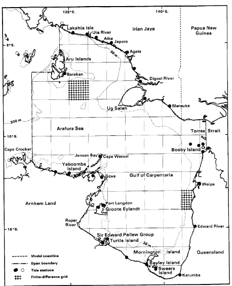
Fig. 1. Plan of the study area, showing the smoothed coastline used in the numerical model.◦Tidal station used to determine the open boundary conditions.•Other tidal stations. Depth contours are shown as dotted lines. Islands whose coastlines are not represented in the model are replaced by water of depth 2.5 m.

3 Numerical solution

In the numerical model, the spherical co-ordinate form of Eq. (7) is replaced by a set of finite difference equations at the vertices of a rectangular grid, using a grid spacing of one eighth of a degree. The boundary condition, Eq. (8), is applied at points where the grid intersects coastlines, the fi-nite difference equations taking into account both the angle between the coastline and the grid and the curvature of the coastline. Both coastline and depths were taken from Admi-ralty charts of the region.

In the original model (Webb, 1981), observed values of the tidal height were imposed on the open boundaries to the west of the Arafura Sea and on the eastern side of Torres Strait. For the new study reported here, the wave entering the region from the west is assumed to have unit amplitude and constant phase all along the western boundary. In the east, Torres Strait is now blocked.

(4)

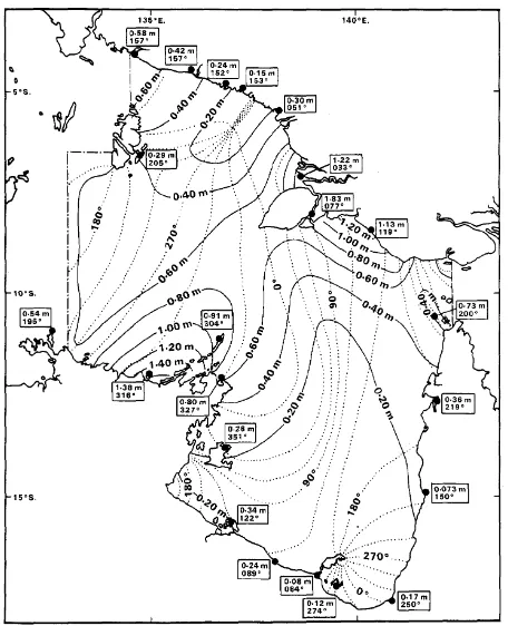
Fig. 2. Computed co-amplitude and co-phase lines for the K1 tide in the Gulf of Carpentaria and Arafura Sea. Observed ampli-tudes and phases, shown in the square boxes, are taken from Easton (1988) and from the Admiralty Tide Tables (Anon, 1971).

are used, the resonance eigenvalues and eigenfunctions are independent of the forcing used for the model.

In the east the original tidal study (Webb, 1981) showed that the amount of tidal energy entering through Torres Strait is small and has little effect on the tides within the Gulf. This might be expected given large differences in tidal phase be-tween the opposite ends of the strait (Anon, 1971) and is con-firmed by the observations of Wolanski et al. (1988). Thus, the decision to simplify the analysis by blocking Torres Strait should have little effect on the large-scale response of the Gulf region.

The coefficients resulting from the finite difference equa-tions are loaded into a sparse matrix and the associated forc-ing terms into a correspondforc-ing vector. The full matrix equa-tion is then solved using Gaussian eliminaequa-tion and back sub-stitution, the numbering of the vertices being organised to minimise the size of the intermediate matrix. Further details of the model and solution are given in Webb (1981).

4 The behaviour at tidal frequencies

Figures 2 and 3, reproduced from Webb (1981), show the original model’s solution for the K1 and M2 tides. In the fig-ures, the amplitude and phase lines are from the model and

Fig. 3. Computed co-amplitude and co-phase lines for the M2 tide. Observed amplitudes and phases, shown in the square boxes, are taken from Easton (1988) and from the Admiralty Tide Tables (Anon, 1971).

the boxed figures show the same quantities measured at tide gauges. There are discrepancies, but they are relatively small. Wolanski (1993) later analysed the tides of the region, mak-ing use of additional current meter data, and found similar tidal patterns. The main difference was for the K1 tide, where the centre of the amphridrome was located 100 km further north.

The present model results for the K1 amplitude and phase lines indicate that, to a first approximation, the diurnal tide propagates along the northern boundary as a Kelvin wave and that it then circles clockwise around the Gulf of Car-pentaria losing energy on the way. However, a simple decay-ing Kelvin wave would have an amplitude which declined monotonically with distance. Instead, the model shows four regions where the amplitude at the coast is a local maximum. Three of these, in corners of the Gulf may result from the Kelvin wave propagating around a nearly right-angled cor-ner. The fourth, in the north-east of the Arafura Sea, near 138◦E, 7◦S, could be associated with a quarter wave reso-nance between the Digoel River3and the shelf edge.

In contrast, the semi-diurnal M2 tide shows no simple re-semblance to a Kelvin wave. In the north of the Arafura Sea, there appears to be a 3/4 wavelength wave, trapped between

(5)

0.0 10.0 20.0 30.0 -4.0

-2.0 0.0 2.0 4.0

radians/day 0.0 10.0 20.0 30.0

-4.0 -2.0 0.0 2.0 4.0

radians/day

Real Imaginary

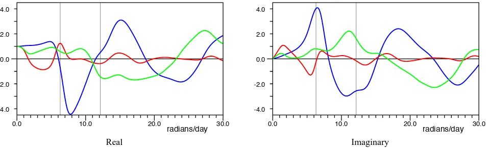
Fig. 4. Real and Imaginary components of the response functions between zero and 30 radians per day for Digoel River (blue), Karumba (red) and Yaboomba Island (green). Vertical lines mark the angular velocities corresponding to the K1 (6.30 radians day−1) and M2 (12.14 radians day−1) tides.

the shelf edge and the Digoel River. There are two additional maxima in the south of the Arafura Sea and the north of the Gulf, which may be related, and a low amplitude east–west oscillation in the centre and south of the Gulf.

These results emphasise the fact that individual tidal con-stituents give little insight into the physical processes in-volved. It is possible to repeat the analysis with other tidal constituents, but the tidal bands are so narrow that little more can be learnt.

However, in the present case the model is not limited to the tidal bands. It can be forced with a wide range of frequencies and so provide a wealth of additional information.

5 The response function

Using the new boundary conditions, the model was run at a series of frequencies between zero and 30 radians per day (∼4.8 cycles per day). It is impractical to show co-tidal charts for all the frequencies calculated, so instead Figs. 4 to 7 show the responseRat three stations which have been selected to illustrate a range of behaviour.Ris defined as

R(x)=ζ (x)/ζb, (9)

whereζ (x)is the (complex) tidal height at positionx, andζb is the tidal height on the open boundary.

The first station is near Digoel River in the north of the Arafura Sea where both the diurnal and semi-diurnal tides indicate the presence of standing waves. The second is near Karumba in the south-east of the Gulf of Carpentaria. Res-onances do not appear to be a key feature of the region, but there is a strong contrast between the diurnal and semi-diurnal tides. The final point is near Yaboomba Island on the southern boundary of the Arafura Sea. The diurnal tide ap-pears as a simple progressive wave along the coast, but the semi-diurnal tide appears to be affected by a resonance.

The results are presented here in three different ways. The first, in terms of the real and imaginary components ofR,

is the most fundamental and is closely related to the later exploration of the complex ω plane. The second, in terms of the amplitude and phase, is easier to relate to the physics, and this is also true of the third, where the real and imaginary components are plotted against each other.

5.1 Real and imaginary components

Figure 4 shows the real and imaginary components of the re-sponse function at each station. As the angular velocity tends to zero, all the real values tend to unity and the imaginary values to zero, indicating that the tide everywhere follows that on the open boundary. As the angular velocity increases, the functions diverge, with the Digoel River showing the largest amplitude excursions. At Karumba the components have much smaller excursions, especially at higher angular velocities. Neighbouring maxima and minima are also much closer than for Digoel River.

At Yaboomba Island the oscillations in the real and imagi-nary components at low angular velocities are less than at the two other stations. However, near 11.5 radians per day there is a change in sign of the real component and a maximum in the imaginary component, after which both components show oscillations comparable with those of Digoel River. 5.2 Amplitude and phase

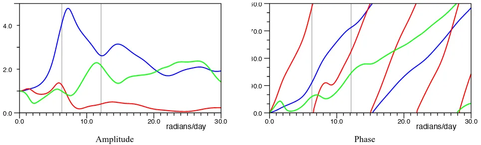
Figure 5 re-plots this data in the form of the amplitude and phase of the response. The amplitudes are all one at zero an-gular velocity, but at higher values the behaviour is very dif-ferent. Thus, over most of the range the Digoel River ampli-tude is above two; it also shows very strong peaks near 7 and 14 radians per day and a weaker broader one near 27 radians per day.

(6)

0.0 10.0 20.0 30.0 0.0

2.0 4.0

radians/day 0.0 10.0 20.0 30.0

0.0 90.0 180.0 270.0 360.0

radians/day

Amplitude Phase

Fig. 5. Amplitude and Phase of the response functions between zero and 30 radians per day for Digoel River (blue) , Karumba (red) and Yaboomba Island (green).

around 30 radians per day, but these are modulated by some structure which may be correlated with the Yaboomba Island response.

The Yaboomba Island station shows a third type of re-sponse. It starts low, and there is a small maximum near 5.5 radians per day, but after a second maximum near 11.5 ra-dians per day, the amplitude stays high and is comparable to that at Digoel River.

The phase plots provide a different insight, in that each of the three curves tends to have a constant slope over all of the frequency range considered. There are changes in slope on the scale of the width of the peaks in the amplitude plot, but except for these features the slope remains remarkably constant.

One possible way to understand this behaviour is to con-sider the response of a simple travelling wave,

ψ=Aexp(ikx−iωt ) . (10)

Assume that the wave speed is constant so that thekequals

ω/c. Then, if this wave is “forced” so that it has amplitude one at the “boundary” wherexis zero, then at distancex, the responseRwill be simply:

R(ω)=exp(ikx) , (11)

=exp(i(x/c)ω) . (12)

In this case the gradient of the phase equalsx/c, the time taken for the wave to propagate from the boundary. Appendix B considers the case of a channel where the depth is not con-stant. This also shows that the phase is a linear function ofω

with the slope again depending on the propagation time. Applying this result to the phases of Fig. 5, it implies that on average incoming waves take about five hours to reach the Yaboomba Island from the open boundary, about ten hours to reach Digoel River and twenty-one hours to reach Karumba. The figures for Yaboomba Island and Karumba are in rough agreement for what might be expected from the phase lines of Figs. 2 and 3. These indicate that, above 10 radians per

day, the tidal wave takes about four hours to reach Yaboomba Island and eighteen to twenty-four hours to reach Karumba.

Estimates for Digoel River are complicated by the stand-ing waves affectstand-ing the semi-diurnal tide, but the diurnal tide indicates about four hours, which is much less than the ten hours estimated from Fig. 5. Thus, the simple idea of a pro-gressive wave appears to be too simple, and an alternative picture needs to be developed.

5.3 Resonance circles

Webb (1973b) discusses the form of the ocean’s response to tidal forcing and shows that it has the form:

ψ (x, ω)=X

j

ψj(x)Aj/(ω−ωj) , (13)

wherex denotes position,ωis the angular velocity, and the eigenvalueωj is the angular velocity of thej-th resonance.

The eigenfunctionψj(x)describes the spacial structure of

the resonance, andAj depends on how the system is forced.

If the resonances are well separated, then near to each res-onance the function at a fixed position has the form:

ψ (ω)=Rj/(ω−ωj)+B(ω) . (14)

whereB(ω)is a smooth background, the contribution of dis-tant resonances.

Letωj have real and imaginary partsωj0andγj. In

phys-ically realistic systems with friction, γj is negative. As ω

moves along the real axis from minus to plus infinity, the res-onance term increases from zero to a value ofiRj/γj when ωequalsωj0, and returns to zero at plus infinity. It is straight-forward to show (Webb, 2011) that as this happens the real and imaginary components move anti-clockwise around a circle that starts at the origin and passes throughiRj/γj at

maximum distance from the origin.

(7)

4.0 2.0

0.0 -2.0

-4.0 0.0 4.0

2.0

-2.0

-4.0

Real

Imaginary

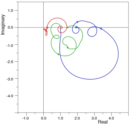
Fig. 6. Polar diagram showing the response functions between zero and 30 radians per day for Digoel River (blue), Karumba (red) and Yaboomba Island (green). The crosses are at intervals of 10 radians per day.

may be difficult. In particular, circles are also produced by delays, such as those produced by the propagation of pro-gressive waves discussed in the last section, but in such cases the circles are centred on the origin.4

To see how well the approach works for the present results, the real and imaginary components are plotted against each other in Fig. 6. All three curves start at the point(1.0+i0.0)

and circle around the origin in an anti-clockwise direction. However, although it is apparent that there are some underly-ing structures present in all three curves, only the Yaboomba Island curve shows anti-clockwise circles, and these are both very small and only occur at low angular velocities.

The main feature of the Karumba curve is that it circles the origin, initially at approximately unit distance, but finally it converges towards the origin. Thus, as discussed before it appears to be primarily a progressive wave which is damped at higher angular velocities.

The Digoel River curve also circles the origin but at a dis-tance which is much greater than one, so this cannot be a simple delay. However, in the absence of an alternative ex-planation, it is possible that the resonances which produce the peaks of Fig. 5 are overlapping or combining in such a way as to produce an effective delay.

Figure 7 shows an attempt to remove the background by adding a linear correction to the phases, such that the total phase change over the whole band is zero. The transforma-tion distorts the resonance circles, the distortransforma-tion being

pro-4_{In terms of the resonance picture, a progressive wave is the} cumulative result of many overlapping resonances.

-4.0 -2.0

-3.0 -1.0

-1.0 0.0 1.0 2.0 3.0 4.0

0.0 1.0

Real

Imaginary

Fig. 7. Polar diagram showing the modified response functions (see text) between zero and 30 radians per day. Colours as in Fig. 6. The crosses are at intervals of 10 radians per day.

portional to the width of the resonance and the magnitude of the linear correction (greatest for Karumba), but the effect is small when the resonances are narrow.

Now all three stations show a series of loops with a posi-tive (anti-clockwise) curvature, as expected from resonances. Karumba and Yaboomba Island both show some small kinks with negative curvature, but these will have been produced by the transformation.

5.4 Analysis of real data

The results of this section show that analysis based on results with real values of the angular velocity is difficult. Plots of just the real or imaginary components as a function of angu-lar velocity are not very useful. Peaks in the amplitude plots start to indicate the presence of resonances, three or four at Digoel River and similar numbers at Yaboomba Island and Karumba but not all at the same angular velocities.

When additional confirmation is looked for in the phases, the main feature appears to be a steady change in phase in-dicating not resonances but delays in the system. The final method, plotting the real and imaginary components against each other, helps to confirm that resonances are being seen at Yaboomba Island, but at the other two stations, interpretation is again difficult.

(8)

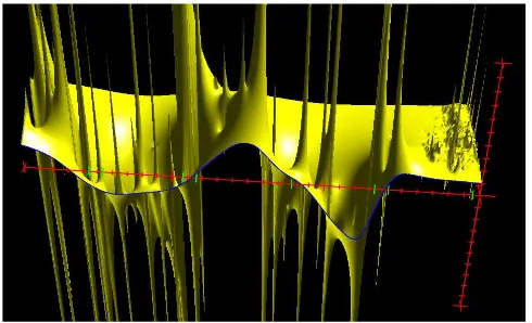
Fig. 8. Real part of the response function at Digoel River plotted as a function of complex angular velocity over the region enclosed by the origin and the points(0−10i),(30−10i)and 30 radians per day. Axes in red with ticks every unit interval. The origin is on the right with the real axis extending to the left and the negative imaginary axis extending backwards. The green ticks indicate the long-period, diurnal, semi-diurnal and higher tidal bands. The blue line is the response at real angular velocities as plotted in Fig. 4 but with the direction of the real axis reversed.

Karumba Yaboomba Island

Fig. 9. Real part of the response functions at Karumba and Yaboomba Island. Details as in Fig. 8.

6 The complexωplane

Figures 8 and 9 show the real component of the response at Digoel River, Karumba and Yaboomba Island plotted as a function of complex angular velocity. The data for the figures

(9)

was then plotted in a view which looks beyond the real axis in the negative imaginary direction.

The values on the real axis are the same as in Fig. 4, but the direction of increasing angular velocity is now towards the left. As discussed in Webb (1973b), the values in the nega-tive real direction (not plotted) are the mirror image of those in the positive direction. This results from the fact that we are using a complex value response function to represent a system in which the input and output functions are both real. The figures show series of mathematical poles at positions corresponding to the complex angular velocities of the reso-nances, the termsωj of Eq. (13). Although it is not always

obvious, the poles are at the same positions in each of the three figures, and, if the resolution was high enough, the re-sponse functions would be seen to extend to plus and minus infinity in the neighbourhood of all of the poles.

The apparent width of each peak depends on the magni-tude of its residue, i.e. the termψj(x)Aj in Eq. (13).

Dif-ferences between the residues in the three figures is thus a measure of the changing importance of each resonance in different locations around the Gulf.

There should be no poles in the positive imaginary direc-tion as these would correspond to modes which grow in time, and, as discussed by Webb (1973b) and in more detail by Nussenzveig (1972), such poles would also break causality. However, although the finite difference scheme used for the model is accurate to second order in the grid spacing, it is not strictly energy conserving, and so it is possible if the er-ror terms are large that it could generate such modes. For the Gulf region this was found not to be the case.

The figures emphasise the large number of resonances found in even a small region of ocean and show that max-ima on the real axis, i.e. in the real world, may not be due to an individual resonance but often result from the combined contributions of a number of resonances.

The figures also show that the resonances fall into two groups with a boundary near four radians per day. At low angular velocities there are a large number of tightly packed resonances, but they have little effect on the response at real values of angular velocity. In this group the residues are small, and there is a large range of decay rates, the imagi-nary components of angular velocity extending to minus ten and beyond.

Above four radians per day, the resonances are well sepa-rated and have much larger residues. At the lower (real) an-gular velocities, the imaginary components are one to two radians per day, and these increase to three to four radians per day for the resonances near thirty radians per day.

This second group of resonances is also the one which ap-pears to have the most influence on the diurnal and semi-diurnal tides. Table 1 contains a list of the resonances closest to the tidal bands plus resonances with low angular velocities which appear to have most effect on the low angular velocity response at Digoel River, Karumba and Yaboomba Island.

6.1 Gravity and rossby waves

Theoretical studies have shown that there are two main classes of long waves in the ocean. The first contains both the gravity waves, found at high angular velocities, and the equatorial and coastal Kelvin waves, which also extend to low angular velocities. In these waves the primary exchange is between the kinetic and potential energy of the wave. The second class of waves consists of the Rossby waves, which are found only at low angular velocities. In these waves the primary exchange is between the two horizontal components of velocity.

Theory also shows that the boundary between the gravity and Rossby waves occurs at an angular velocity of f, the Coriolis parameter,

f =2sin(θ ) , (15)

where θ is latitude, and is the angular velocity of the Earth. Waves with angular velocities near f are likely to show a mixture of both properties (Longuet-Higgins, 1968; Longuet-Higgins and Pond, 1980).

The Gulf of Carpentaria and the Arafura Sea span latitudes between 5◦S and 18◦S. This corresponds to values of the Coriolis parameterf, between 1.1 and 3.6 radians per day. Thus, the change in properties seen near 4 radians per day can be identified as being due to the change from the Rossby wave to the gravity wave parts of the spectrum.

If Eq. (1) is used to study the decay of a steady current, it is easy to show that the decay rate is proportional toκ/ h, where

κ is the friction parameter andhthe depth. Webb (2011) in-vestigated gravity wave resonances in a simple 1-D model with a constant depth continental shelf and showed that the resonance decay rates, the imaginary parts of the complex angular velocity, were given by the same equation.

In the present model,κ has the value 0.1 cm s−2, and the depths range from over 100 m in parts of the Arafura sea and 70 m in the centre of the Gulf of Carpentaria to 20 m and less near to the coastline. Using the above equation, a depth of 100 m gives a decay rate of 0.86 day−1and this increases to 1.73 day−1for a depth of 50 m, 3.46 day−1for 25 m and 8.64 day−1for 10 m. The gravity wave values of Table 1 are thus consistent with mean depths of between 25 and 50 m, values which are not unreasonable.

(10)

Resonance aa Resonance A

135.0 140.0

-15.0 -10.0 -5.0

Longitude

Latitude

135.0 140.0

-15.0 -10.0 -5.0

Longitude

Latitude

Fig. 10. Amplitude and phase contours for resonances aa and A (Table 1). The phase contours (light) are at intervals of 30 degrees, colour coded with red in the quadrant−180◦to−90◦, brown−90◦to 0◦, green 0◦to 90◦and blue 90◦to 180◦. Amplitude is is in the range 0 to 1, with contours (heavy) at intervals of 0.2 and darker colours indicating greater amplitude. Amplitude is zero on the open (western) boundary and at the centre of amphidromes, and has the value 1 at points with maximum amplitude.

Table 1. Real and Imaginary components of angular velocity (in radians per day) for some of the key resonances, plus the names used to refer to them in the text.

Angular velocity Angular velocity

Real Imag. Real Imag.

aa 1.4561 −1.1419 K 15.3736 −1.6588

bb 3.1370 −1.6373 L 16.7251 −2.0066

A 5.8397 −1.1277 M 16.9845 −3.5121

B 7.0215 −1.3056 N 17,4437 −3.2135

C 7.8389 −2.0418 O 18.4964 −2.6164

D 9.5938 −2.0780 P 19.1721 −2.7670

E 10.2025 −2.6180 Q 20.0978 −3.4472

F 11.4272 −1.7270 R 20.4820 −1.8994

G 12.6226 −2.4655 S 20.6322 −3.3178

H 13.3884 −2.2500 T 21.4129 −1.9414

I 14.1413 −2.2405 U 22.5463 −2.6505

J 14.8486 −2.5489

7 The resonances

The angular velocities of the resonances can be found by fit-ting Eq. (14) to one of the calculated response functions in the neighbourhood of each resonance. Use was made of the

four nearest calculated values and these were fitted using a linear background,

ψ (ω)=Rj/(ω−ωj)+A+B ω . (16)

As discussed in Appendix A, this can be converted into a lin-ear matrix equation and so solved for the unknowns including the resonance frequencyωj. The results for the main

reso-nances using the data from Digoel River are given in Table 1. The results obtained from using any of the other stations are essentially the same.

Once the angular velocity of a resonance is known, the spatial structure, the eigenfunction of the matrix equation, can be calculated in a similar manner. This time, solutions to the model equations were obtained for each of the four angular velocitiesωj±δωandωj±ıδω, whereδωequalled

(11)

Resonance B Resonance C

135.0 140.0

-15.0 -10.0 -5.0

Longitude

Latitude

135.0 140.0

-15.0 -10.0 -5.0

Longitude

Latitude

Resonance D Resonance E

135.0 140.0

-15.0 -10.0 -5.0

Longitude

Latitude

135.0 140.0

-15.0 -10.0 -5.0

Longitude

Latitude

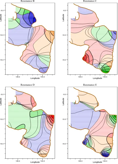
Fig. 11. Amplitude and phase contours for resonances B, C, D and E. Contours as in Fig. 10.

7.1 Resonance waveforms

Figures 10 to 13 show the amplitude and phase of some of the main resonances affecting the diurnal and semi-diurnal tides

(12)

Resonance F Resonance H

135.0 140.0

-15.0 -10.0 -5.0

Longitude

Latitude

135.0 140.0

-15.0 -10.0 -5.0

Longitude

Latitude

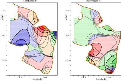
Fig. 12. Amplitude and phase contours for resonances F and H. Contours as in Fig. 10.

velocity is less than the Coriolis parameter everywhere ex-cept near the northern coastline of the Arafura Sea. As a re-sult its properties are those of a Rossby wave with only a small fraction of its energy in the form of potential energy. Thus, even at low angular velocities it has only a limited ef-fect on tidal height5.

The remaining resonances illustrated are all primarily gravity wave modes, and as such each of them might domi-nate the response with a suitable pattern of forcing. However, in the present case the forcing is limited to the shelf edge, and this appears to limit the importance of individual resonances and the way they interact.

At low angular velocities, resonances “A”, “B” and “C” are well separated in angular velocity from other resonances and are relatively weakly damped. As a result one might expect them to dominate the response in the diurnal tide band, and, as discussed later, this is the case.

Figures 10 and 11 show that resonances “A” and “C” are both primarily progressive waves trapped within the Gulf of Carpentaria. Their angular velocities appear to be deter-mined by “A” fitting a single wavelength around a single amphidrome and “C” two wavelengths around a double am-phidrome.

In contrast resonance “B” (Fig. 11) is primarily a quar-ter wavelength wave trapped between the shelf edge and the

5_{Grignon (2005) showed that the fundamental mode of the} En-glish Channel has similar properties

Digoel River. Some energy does propagate into and circu-late around the Gulf of Carpentaria, but it appears to be the distance between the shelf edge and the Digoel River which determines the angular velocity of this mode. The angular velocities of resonances “B” and “C” are very close, so it is possible that this results in some mixing of the solutions.

At higher angular velocities the structure of the resonances becomes more complex, and it is more difficult to relate them to physical features. One exception is resonance “F”, which appears to be primarily a standing wave trapped between the northern boundary of the Gulf of Carpentaria and the south-ern boundary of the Arafura Sea. Another is resonance “I”, which is a three-quarters wave trapped between Digoel River and the shelf break. Note that this time there is very little coupling to the Gulf of Carpentaria.

The remaining resonances have a more irregular structure. Many of them, like resonance “E”, have maxima in corners of the Gulf of Carpentaria, but the increasingly complex pat-tern of phases indicates that their main role is to provide the complete set of functions required to describe all possible wave patterns.

7.2 Comparison with a simpler model

(13)

135.0 140.0 -15.0

-10.0 -5.0

Longitude

Latitude

Fig. 13. Amplitude and phase contours for resonance I. Contours as in Fig. 10.

resonances had periods of 16.4, 10.4 and 7.9 h, correspond-ing to 9.2, 14.5 and 19.1 radians per day, respectively. The results were given some support by Melville and Buchwald (1976), who analysed sea level records from the Gulf of Car-pentaria.

One might have expected the Buchwald and Williams (1975) resonances to show similarities with those of the present study, which are most energetic in the Gulf of Car-pentaria. The best examples are resonances C and E, but these have angular velocities of 7.8 and 10.2 radians per day and do not correspond to any of the Buchwald and Williams (1975) values. This is most likely due to the lack of a Coriolis term in the earlier study.

8 Resonances and real angular velocities

The polar plots, discussed earlier, showed that at real val-ues of the angular velocity the presence of resonances could be indicated by the presence of tight loops in the response function. Here, use is made of this property to identify the resonances responsible for the key features of the response function in the diurnal and semi-diurnal bands. Over such a band, it should be possible to expand the response function

R(x, ω)at sitexas:

R(x, ω)=X

j

Rj(x)/(ω−ωj)+c.c.+B(x, ω) , (17)

Program: occam/tides/gulftides/src/plot_f5.F

-5.0 -4.0 -3.0 -2.0 -1.0 0.0 1.0 2.0 3.0 4.0 5.0 -5.0

-4.0 -3.0 -2.0 -1.0 0.0 1.0 2.0 3.0 4.0 5.0

Real

Imaginary

Digoul River

Response curve, lower limit = 0.0000 Response curve, upper limit = 9.0000 Resonance sum, lower limit = 5.0000 Resonance sum, upper limit = 8.0000

B B

5

8

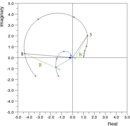
Fig. 14. Polar plot of response function (black) at Digoel River, for the range 0 to 9 radians per day. The black crosses are at intervals of one radian per day. The contribution of the resonance “B”, and its conjugate pole (defined in the text), is plotted in green at 5 and 8 radians per day, the conjugate contribution being the smaller. The residual after subtracting the contribution of resonance “B” and its conjugate pole is plotted in blue, also for the range 0 to 9 radians per day.

where the sumjis over a limited number of key resonances, andB(x, ω)is a smooth background.Rj(x)andwj are the

values calculated in the previous section. The term c.c. rep-resents the contributions from the conjugate set of poles, with eigenvalues−ω_j∗ and eigenfunctions−R_j∗(x), needed for symmetry (Webb 1973b, Appendix I).

The choice of key resonances is to a certain extent subjec-tive. In the examples given here, it was done by finding a set of resonances which, over the band of real angular veloci-ties considered, reproduced the main features of the response function and left a residual which was small and smooth. As a final check the other nearby resonances were each added in turn but then left out if they did not significantly smooth or reduce the residual.

(14)

-2.0 -1.0 0.0 1.0 2.0

Real

Imaginary

Response

Karumba

aa A

B aa A B

5 8

Fig. 15. Polar plot of response function (black) at Karumba, for the range 0 to 9 radians per day. The black crosses are at intervals of one radian per day. The contribution of the resonances “aa” (red), “A” (yellow) and “B” (green), and their conjugate poles, are plotted at 5 and 8 radians per day, the conjugate contribution being the smaller. The residual, after subtracting the contributions of these resonances and their conjugates, is plotted in blue, also for the range 0 to 9 ra-dians per day.

Two bands of angular velocities are considered. The first extends from zero to nine radians per day. This covers the diurnal tides and also shows the behaviour at very low val-ues of angular velocity. The second band extends from ten to fifteen radians per day and covers the semi-diurnal tides. 8.1 The diurnal band

The result for Digoel River, for the band 0 to 9 radians per day is shown in Fig. 14. The large amplitude loop in the re-sponse function can all be explained by the changing ampli-tude and phase of the contribution of resonance “B”, a quar-ter wavelength resonance. The background quar-term is seen to grow with angular velocity, reaching an amplitude of two by 8 radians per day, but it still remains much smaller than the single resonance contribution.

The corresponding result for Karumba is shown in Fig. 15. At low angular velocities it was found necessary to include resonance “aa” in order to reduce the background at near zero angular velocity. For the 5 to 8 radians per day region, which includes the diurnal tides, it was found necessary to include both “A” and “B” resonances. These both have large ampli-tudes and phase changes of around 90◦.

More importantly they have approximately opposite phase. Near 5 radians per day, the contribution from reso-nance “A” is large and “B” only reduces it slightly.

How-Program: occam/tides/gulftides/src/plot_f5.F

0.0 1.0

Real

Imaginary

Response

Yarumba Island

aa

A B D

F

aa _A

B D

F

5 8

Fig. 16. Polar plot of response function (black) at Yaboomba Is-land, for the range 0 to 9 radians per day. The black crosses are at intervals of one radian per day. The contribution of the resonances “aa” (red), “A” (yellow), “B” (light green), “D” (dark green), and “F” (purple), and their conjugate poles, are plotted at 5 and 8 radi-ans per day, the conjugate contribution being the smaller. The resid-ual, after subtracting the contributions of these resonances and their conjugates, is plotted in blue, also for the range 0 to 9 radians per day.

ever, by 8 radians per day they are effectively cancelling each other out, and this results in a much lower amplitude response function. Figures 2 and 3 show that the semi-diurnal tides at Karumba are low compared with the diurnal tides, and this might have been thought to be a result of an increase in the effect of friction at higher angular velocities. However, in the present case both modes have similar decay times, and so the reduction in amplitude is purely an effect of interference between the two modes.

A further complication is found is found in the results for Yaboomba Island (Fig. 16). The first loop is found to be pri-marily the effect of the Rossby wave resonance “aa”. Reso-nances “A” and “B” are also significant. They again show an approximately 90◦_{phase change between 5 and 8 radians per}

(15)

-4.0 -3.0 -2.0 -1.0 0.0 1.0 2.0 3.0 4.0

Real

Imaginary

Digoul River

B D

F H

I P

B D F H I

P

11

14

Fig. 17. Polar plot of response function (black) at Digoel River, for the range 10 to 15 radians per day. The black crosses are at inter-vals of one radian per day. The contribution of the resonances “B”, “D”, “F”, “H”, “I”, and “P”, and their conjugate poles, are plot-ted at 11 and 14 radians per day, the conjugate contribution being the smaller. The residual, after subtracting the contributions of these resonances and their conjugates, is plotted in blue, also for the range 10 to 15 radians per day.

8.2 The semi-diurnal band

Figure 17 shows the response function at Digoel River in a range including the semi-diurnal tides. Resonance “B” is still significant, but it is declining in importance and a large number of other resonances are now involved. These include “D”, “F”, “H” and “P”, all of which show noticeable phase changes between 11 and 14 radians per day, but the largest contribution is now from “I”, the three-quarter wave reso-nance trapped between the Digoel River and the shelf edge.

At Karumba, Fig. 18, all of the resonances in the range “D” to “K” now make significant contributions. The largest am-plitude term is that of “H”, a rather complex resonance con-fined to the Gulf, but its effect is to a large extent cancelled out by other resonances. However, its increased amplitude does seem to be responsible for the second partial loop seen around 14 radians per day.

Cancellation is also seen within the group of resonances “E”, “F”, and “G”. Resonances “A”, “B”, and “C” (which for clarity are not plotted) cancel each other in a similar manner. In contrast to Digoel River and Karumba, the number of significant resonances contributing to the response function at Yaboomba Island has dropped (see Fig. 19). “F” is the largest resonance, responsible for the main loop, and only two more, “D” and “K”, are required to smooth the

back-Program: occam/tides/gulftides/src/plot_f6.F

-1.0 0.0 1.0

Real

Imaginary

Karumba D

E

F G

H I J K

D _E

F G

H I

J K 11

14

Fig. 18. Polar plot of response function (black) at Karumba, for the range 10 to 15 radians per day. The black crosses are at intervals of one radian per day. The contribution of the resonances “D” to “K”, and their conjugate poles, are plotted at 11 and 14 radians per day, the conjugate contribution being the smaller. The residual, after sub-tracting the contributions of these resonances and their conjugates, is plotted in blue, also for the range 10 to 15 radians per day.

ground. The result confirms that the unusual standing wave between the southern boundary of the Arafura Sea and the northern boundary of the Gulf of Carpentaria is a key feature of the region.

9 Conclusions

The results demonstrate the advantages of linearised tidal models which can work with complex values of angular ve-locity. In reality non-linear processes occur in the ocean, but although locally they may be important, the large scale re-sponse of the ocean to tidal forcing is predominantly linear. Of course the linearisation process needs to be done care-fully, and if possible validated, but it does provide a different viewpoint for the study of the ocean.

(16)

-2.0 -1.0 0.0 1.0 2.0

-1.0 0.0 1.0 2.0

Real

Imaginary

Response

Yarumba Island D

F

K

D _F

K 11

14

Fig. 19. Polar plot of response function (black) at Yaboomba Is-land, for the range 10 to 15 radians per day. The black crosses are at intervals of one radian per day. The contribution of the resonances “D”, “F” and “K”, and their conjugate poles, are plotted at 11 and 14 radians per day, the conjugate contribution being the smaller. The residual, after subtracting the contributions of these resonances and their conjugates, is plotted in blue, also for the range 10 to 15 radi-ans per day.

wave only slightly modified by other processes. The polar diagrams were more informative as they showed a number of tight loops with positive curvature. Theory predicts that isolated resonances will generate such loops.

In principle it should be possible go further by analyti-cally continuing the response function from the real axis to complex values of angular velocity. However, such a process can be affected by numerical noise and so is likely to be prac-tical only for well separated resonances close to the real axis. When the restriction was lifted and the model run for com-plex values of angular velocity, the results were much more informative, the three dimensional figures showing a com-plex pattern of resonances. This included a series of poles with large residues extending from six radians per day to higher angular velocities. These were identified as the grav-ity wave resonances of the region. There was also a field of smaller poles with small real angular velocities but with a large range of imaginary angular velocities. These were iden-tified as the Rossby wave modes.

An investigation of the eigenfunctions showed that some of the gravity modes, especially those with low (real) an-gular velocities, could be identified as fundamental 1/4 or 3/4 wavelength modes fitting between the shelf edge and the coast or modes associated with reflection between opposing boundaries. Others were much more complex, whose main

role may be to contribute to the complete set of modes needed to describe all possible waveforms within the system.

The Rossby wave modes were not investigated in the same way, but one of them was found to be a 1/4 wavelength wave trapped between the shelf edge and the southern boundary of the Gulf of Carpentaria. With no Coriolis term this would be the fundamental quarter wavelength mode of the system and so would have a significant impact on the sea level response. However, here it is at such a low angular velocity that it is primarily a Rossby wave and, except near Yaboomba Island where the other terms are small, it has limited impact on the sea level response.

These results were then used to reinterpret the response functions calculated on the real axis. This showed that there is no band of real angular velocities where the response can be represented by the contribution from a single resonance. However, close to the diurnal tidal band there are only a few resonances, and, although a background term is also re-quired, these were found to dominate the response within the band. There are more resonances close to the semi-diurnal band, and the behaviour there was found to be more compli-cated.

The results also show that in both bands there are regions of the continental shelf where the response is strongly influ-enced by resonances trapped between the shelf edge and the coast or between two opposing coastlines. Elsewhere the res-onances often appear to produce cooperative effects, a group of resonances forming a single “resonant like” loop, can-celling each others contributions or producing an approxi-mation to a simple progressive wave.

This apparent cooperation may simply reflect the fact that in such regions the separation between resonances is less than their distance from the real axis. Alternatively, it may be an indication that, where it occurs, the physical process involved is one for which a simple resonance interpretation is the wrong one. This should occur, for example, in the case of a simple progressive wave. The resonance picture may also be inappropriate for a slowly narrowing channel many wavelengths long, for which a Wentzel–Kramers–Brillouin (WKB) type approximation may be more relevant. However, the fact that the 1/4, 3/4 and other simple resonances stand out so clearly implies that such resonances are still likely to be important in other regions of the world’s ocean.

(17)

Appendix A

Resonance and background

The problem is to fit a series of response function values

R(ωi)for different values of ωi by a single resonance and

a linear background,

R(ωi)=Rj/(ωi−ωj)+P+Q ωi. (A1)

P andQare complex constants,ωj is the complex

angu-lar velocity of the resonance, andRj its residue. This is a

specific form of the more general problem of fitting a set of valuesyiandxi to an equation of the form:

y=A/(x−B)+

N X

n=0

Cnxn. (A2)

Multiplying by(x−B),

y(x−B)=A+

N X

n=0

(Cnxn+1−CnBxn) , (A3)

yx=A+By−C0B

+ N X

n=1

(Cn−1−CnB)xn+CNxN+1,

yx=(A−C0B)+By

+ N X

n=1

(Cn−1−CnB)xn+CNxN+1.

This can be written in the form:

yx=D0y+ N+2

X

n=1

Dnxn−1. (A4)

This, like Eq. (A2), has N+3 unknowns. If a similar num-ber of pairs of valuesxandyare available, it gives a matrix equation which can be solved using standard methods for the unknownsD. Then

B =D0, (A5)

CN =DN+2,

Cn−1=Dn+1+CnB for n=1 . . . N ,

A=D1+C0B .

If in Eq. (A1) the angular velocity of the resonanceωj is

known, then Eq. (A2) can be rewritten in the form:

y=A/x0+

N X

n=0

C_n0x0n, (A6)

wherex0 now equals (wi−wj). Dropping the primes, the

equivalent of Eq. (A4) is:

yx=

N+1 X

n=0

Dnxn. (A7)

In matrix form, the set of equations become:

MD=F, (A8)

where M is a matrix, andDandF are vectors,

Mm,n=xmn, Fm=ymxm.

M is a Vandermonde matrix. Turner (1966) shows that its inverse, M−1, contains terms which are simple functions of the variablesxm. The solution is then given by

D=M−1F. (A9)

The residue of the pole in Eq. (A6) is given byD0. In the case of four unknowns, if thexis have the values±δand±iδ,

whereδis non-zero, then the residue is just the mean value of the elements ofF.

Appendix B

Shallow water solution in a channel

Consider a channel of constant width where the depthH (x)

varies with distancex along the channel. The shallow water equations are then:

du/dt = −gdh/dx ,

dh/dt = −d(H u)/dx , (B1)

wherehis sea level,uis velocity,tis time, andgis gravity. If the waves have constant angular velocityω, then after elimi-natinguand dropping the time dependent term, exp(−iωt ),

h00+(H0/H )h0+(ω2/(gH ))h=0, (B2)

whereh0 andh00 represent dh/dx and dh2/dx2. Letkequal

(ω2/(gH ))1/2. It has the properties of a local wavenumber. Then

h00−(2k0/ k)h0+k2h=0. (B3)

If the depth changes slowly over each wavelength, a method similar to the WKB approximation can be used (Gill, 1982). Let

h(x)=A exp(iφ (x)). (B4)

Substitute in Eq. (B3), equate the real and imaginary com-ponents and simplify:

φ02=k2+ [A00/A−2(k0/ k)(A0/A)],

2A0k0=A (2(k0/ k)φ0−φ00). (B5)

If the amplitude and the depth change slowly so that the term in square brackets is small,

φ0≈ ±k,

(18)

whereCis a constant. Thus

h(x)≈Ck(x)1/2exp(±i

Z

k(x)dx),

≈Ck(x)1/2exp(±iω

Z

(gH (x))−1/2dx). (B7)

At a fixed point along the channel, the phase of the solution is linearly proportional to the angular velocity of the wave.

Acknowledgements. I wish to thank the editors of the CSIRO journal “Marine and Freshwater Research” for permission to reuse figures from Webb (1981).

Edited by: J. M. Huthnance

References

Anon: Admiralty Tide Tables, Hydrographer of the Navy, London, 1971.

Arbic, B. K. and Garrett, C.: A coupled oscillator model of shelf and ocean tides, Cont. Shelf Res., 20, 564–574, doi:10.1016/j.csr.2009.07.008, 2010.

Arbic, B. K., St-Laurent, P., Sutherland, G., and Garrett, C.: On the resonance and influence of the tides in Ungava Bay and Hudson Strait, Geophys. Res. Lett, 34, L17606, doi:10.1029/2007GL030845, 2007.

Arbic, B. K., Karsten, R. H., and Garrett, C.: On Tidal Resonance in the Global Ocean and the Back-Effect of Coastal Tides upon Open-Ocean Tides, Atmos.-Ocean, 47, 239–266, 2009. Buchwald, V. T. and Williams, N. V.: Rectangular resonators on

infinite and semi-infinite channels, J. Fluid Mech., 67, 497–511, 1975.

Duff, G.: Tidal resonance and tidal barriers in the Bay of Fundy system, J. Fish. Res. Board Can., 27, 1701–1728, 1970. Easton, A. K.: The tides of the continent of Australia, Report 37,

Horace Lamb Centre for Oceanographic Research, Flinders Uni-versity of South Australia, 1988.

Egbert, G. and Ray, R.: Semi-diurnal and diurnal tidal dissipation from TOPEX/Poseidon altimeter data, Geophys. Res. Lett., 30, 1907, doi:10.1029/2003GL017676, 2003.

Fong, S. and Heaps, N.: Note on the quarter-wave tidal resonance in the Bristol Channnel, Institute of Oceanographic Sciences, Re-port No., 63, 1978.

Garrett, C. and Munk, W.: The age of the Tide and the ’Q’ of the Ocean, Deep-Sea Res., 18, 493–504, 1971.

Gill, A.: Atmosphere-Ocean Dynamics, Academic Press, New York & London, 662 pp, 1982.

Green, J. A. M.: Ocean tides and resonances, Ocean Dynam., 60, 1243–1253, 2010.

Griffiths, S. D. and Peltier, W. R.: Megatides in the Arctic Ocean under glacial conditions, Geophys. Res. Lett., L08605, doi:10.1029/2008GL033263, 2008.

Griffiths, S. D. and Peltier, W. R.: Modeling of Polar ocean Tides at the Last Glacial Maximum: Amplification, Sensitivity, and Cli-matological Implications, J. Climate, 22, 2905–2924, 2009. Grignon, L.: Tidal resonances on the North-West European Shelf,

Master’s thesis, University of Southampton, School of Ocean and Earth Science, 2005.

Longuet-Higgins, M.: The Eigenfunctions of Laplace’s Tidal Equa-tions over a Sphere, Philos. Trans. Roy. Soc., A262, 511–607, 1968.

Longuet-Higgins, M. and Pond, G. S.: The Free Oscillations of Fluid on a Hemisphere Bounded by Meridians of Longitude, Phi-los. Trans. Roy. Soc., A266, 193–223, 1980.

Melville, W. and Buchwald, V.: Oscillations of the Gulf of Carpen-taria, J. Phys. Oceanogr., 6, 394–398, 1976.

Miller, G. R.: The flux of tidal energy out of the deep ocean, J. Geophys. Res., 71, 2485–2489, 1966.

M¨uller, M.: Synthesis of forced oscillations, Part 1: Tidal dynamics and the influence of the loading and self-attraction effect, Geo-phys. Res. Lett., 34, L05606, doi:10.1029/2006GL028870, 2007. Nussenzveig, H. M.: Causality and Dispersion Relations, Academic

Press, 1972.

Turner, L. R.: Inverse of the Vandermonde Matrix with Applica-tions, NASA Technical Note D-3547, US National Aeronautics and Space Administration, 1966.

Webb, D.: On the Age of the Semi-diurnal Tide, Deep-Sea Res., 20, 847–852, 1973a.

Webb, D. J.: Green’s Function and Tidal Prediction, Rev. Geophys. Space Phys., 12, 103–116, 1973b.

Webb, D. J.: A Model of Continental Shelf Resonances, Deep-Sea Res., 23, 1–15, 1976.

Webb, D. J.: Numerical Model of the Tides in the Gulf of Carpen-taria and Arafura Sea, Austr. J. Mar. Freshw. Res., 32, 31–44, 1981.

Webb, D. J.: Tides and Tidal Energy, Contemp. Phys., 23, 419–442, 1982.

Webb, D. J.: Notes on a 1-D Model of Continental Shelf Reso-nances, Research and Consultancy Report 85, National Oceanog-raphy Centre, Southampton, available at: http://eprints.soton.ac. uk/171197, 2011.

Wolanski, E.: Water Circulation in the Gulf of Carpentaria, J. Mar. Syst., 4, 401–420, 1993.

Wolanski, E., Ridd, P., and Inoue, M.: Currents through Torres Strait, J. Phys. Oceanogr., 18, 1535–1545, 1988.