http://www.sciencepublishinggroup.com/j/ajam doi: 10.11648/j.ajam.20190701.13
ISSN: 2330-0043 (Print); ISSN: 2330-006X (Online)
Modified Model and Stability Analysis of the Spread of
Hepatitis B Virus Disease
Birke Seyoum Desta, Purnachandra Rao Koya
*Department of Mathematics, Hawassa University, Hawassa, Ethiopia
Email address:
*Corresponding author
To cite this article:
Birke Seyoum Desta, Purnachandra Rao Koya. Modified Model and Stability Analysis of the Spread of Hepatitis B Virus Disease. American Journal of Applied Mathematics. Vol. 7, No. 1, 2019, pp. 13-20. doi: 10.11648/j.ajam.20190701.13
Received: June 18, 2018; Accepted: April 28, 2019; Published: May 29, 2019
Abstract:
In this study the infected population is classified into two categories viz., chronic and acute and thus developed a five compartmental SEICIAR model. Also, both vaccination and treatments are included and studied their impact on the spreadof hepatitis B virus. The present model is biologically meaningful and mathematically well posed since the solutions are proved to be positive as well as bounded. The basic reproduction number RO of the model is derived using the next generation
matrix method. Further, the equilibrium points of the model are identified and mathematical analysis pertaining to their stability is conducted using Routh – Hurtiz criteria. It is shown that the disease free equilibrium point is locally and globally stable If RO<1. On the other hand, the endemic equilibrium point is proved to be stable if RO>1. Also, the numerical simulation study of the model is carried out using ode45 of MATLAB: Rung – Kutta order four. It is observed that, if the vaccination and treatment rates are increased then the infective population size decreases and evenfall to zero over time. Hence, it is concluded that the use of vaccination and treatment at the highest possible rates is essential so as to control the spread hepatitis B virus.
Keywords:
Hepatitis B Virus, Vaccination, Treatment, Mathematical Model, Basic Reproduction Number, Stability Analysis, Numerical Simulation1. Introduction
Hepatitis is an infectious disease that causes inflammation of the liver in human body. This disease is divided into five categories of which one is hepatitis B and it is caused by the hepatitis B virus. The hepatitis B infections occur only if the virus is able to enter the blood stream and reach the liver. In the liver the virus reproduces large numbers of virus and releases into blood streams [1]. The hepatitis B infection is categorized into two types:(i) Acute hepatitis B which has no treatment so far and (ii) Chronic hepatitis B which has treatment.
The acute hepatitis B infection can range in severity from a mild illness with few or no symptoms to a serious condition requiring hospitalization. For those who are affected by this disease, the doctors usually recommend rest, adequate nutrition, fluids, and close medical monitoring. However, there is no medical treatment for this disease but only
supportive care [7].
In contraction, there are several approved medications to treat a person who is infected by chronic hepatitis B virus [1]. The chronic HBV infection has some complications including cirrhosis or primary liver cancer.
The spread of HBV is one of the major health problems in the world. It is a major cause of mortality and morbidity globally. According to WHO (2015) over one – third of the world’s population i.e., more than 2 billion people, have been or are actively infected with HBV and of which 257 million persons are living with chronic HBV infection in the world [2]. However, one million people die each year due to this disease. More than 90% of infected adults will recover naturally within the first year of infection even though some of them will not even show any symptoms of the disease [3].
largest number of chronic HBV carriers, after Asia, and is considered as highly endemic. The Africa and western pacific regions accounted for 68% of the infected [2].
In Ethiopia, hepatitis B affects 240 million people. Each year an estimated 650000 people die from liver disease or liver cancer caused by HBV [5].
Hepatitis B virus is transmitted in many ways. The virus is found in the blood or certain body fluids and is spread when blood or body fluid from an infected person enters the body of a person who is not infected. This can occur in a variety of ways including: sex with an infected person;blood to blood product; and shared syringes, razors and brushes; mothers can pass the infection to their children during pregnancy or breast feeding; contact with wounds or skin sores; when an infected person bites another person; pre-chewing food for babies [6, 7].
Many people with hepatitis B do not have symptoms and do not know that they are infected [1]. If symptoms occur, they can include: fever, feeling tired, not wanting to eat, upset stomach, throwing up, dark urine, grey – colored stool, joints pain, yellow skin and eyes.
Moneim and Khalil (2015) study modeling and simulation of the spread of HBV disease with infectious latent. The authors also studied the global behavior of the spread of the disease using a SEIR model with a constant vaccination rate. It is assumed that the infectivity during the incubation period is considered as a second way of transmission. The basic reproduction number is derived as a function of the two contact rates and . The disease free equilibrium point of the model is found and shown that it is asymptotically stable
if < 1. On the other hand, the endemic equilibrium point
is stable if > 1andthat the disease is persisted in the population. Simulation study of the model has been conducted with varying vaccination parametric values [8]. However, there are some gaps in that study: the authors considered both the acute and chronic infected populations as belong to one compartment; also the study did not consider the treatment.
In the present research, the authors considered that the acute and the chronic infected populations belong to two separate compartments. Thus, the gaps left in the study [8] are filled by replacing modelwith a model. That is, in the new and present model the whole human population is divided in to five compartments: susceptible ; exposed ; chronic infective ; acute infective ; and recovered . Also the present study considers both vaccination and treatment so as to prevent the spread of HBV.
2. Mathematical Formulation of the
Model
The present mathematical model is aimed to help in understanding the dynamics and spread of hepatitis B virus diseases. In this section, a five compartmental model is formulated based on the deterministic approach. Also the model assumptions and flow diagram are
included. Further, the validity of the model is verified by proving that all the model variables are both positive and bounded. The disease free equilibrium point, endemic equilibrium point and the basic reproduction number of the model are found.
2.1. Model Assumptions
The modified modelof the present study is constructed based on the following assumptions:
The population is divided into five classes: the susceptible ; the exposed ; the chronic infective ; the acute infective ; and the recovered .
Age, sex, social status and race do not affect the probability of getting infected.
A susceptible individual can be infected only by contacting with infectious individuals.
There is vaccination for newly born babies against hepatitis B.
The chronic carriers are treated.
Acute infections are not subjected to treatment. But, some of them are cured due to natural immunity.
The exposed individuals are not infectious. That is, they are not capable of transmitting virus.
The susceptible population has not yet infected by the disease but likely to get infected infuture. Susceptible population increases due to recruit men to find ividuals with a rate 1 − but, reduces due to natural death with a rate μ.
The exposed population comprises of those individuals who are infected but not yet infectious i.e., they are not capable of transmitting virus. This shows that the transmission rate of the HBV disease is assumed to be the contact rate between the susceptible and the infective [9]. The exposed class grows with the incidence rate + ⁄ but decreases due to the natural death rate of μ, due to transfer to with a rate , and due to transfer to
with a rate .
The chronic infective class comprises those individuals who are infected and also capable of transmitting the disease. But, this category population has medical treatment. Chronic infective class grows with a rate as people flow in fromthe exposed class but decrease due to natural death rate μ, death rate due to disease and by treatment rate .
Acute infective class comprises of those who are infected and also capable of transmitting the disease. Acute infections are not subjected to antiviral treatment but some of them have the possibility of being cured due to natural immunity [10]. Size of this class increases by a rate as people flow in from exposed class. But, the class size decrease due to natural death rate μ, death due to virus at the rate and at recovered rate .
Finally, removed class increases due to a successful cure of chronic infected patients at the treatment rate ; vaccinated population with a rate ; and cure of acute infected patients due natural immunity at rate . Further, the population size decreases due to natural death rate µ.
Table 1. Descriptions of parameters and variables used in model equations.
Parameter /Variable Description
Size of susceptible population Size of exposed population Size of chronic infective population Size of acute infective population Size of recovered population Size of the total population Transmission rate from to Transmission rate from to Recruitment rate
Death rate in due to disease Treatment rate of
Recovered rate of Rate of transfer from to Rate of transfer from to Natural death rate
Death rate in due to disease
Vaccination rate
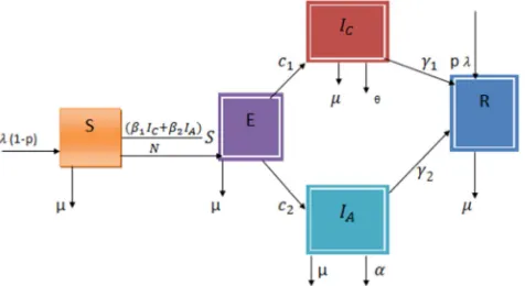
The compartmental flow chart showing the compartments and flow directions of people is given in Figure 1. In that figure, the variables, parameters and recruitment, treatment, vaccination, transfer and death rates are also indicated.
Figure 1. Flow diagram for model.
Including the model assumptions and flow of the people shown in the model diagram, the system of ODE equations representing the model can be constructed as follows:
⁄ ! 1 ⁄ – (1)
⁄ ! ⁄ μ (2)
⁄ ! (3)
⁄ ! #$% (4)
⁄ ! μ (5)
Here, in (1) to (5) the total population size is denoted by and hence ! . 2.2. Positivity of the Solution In order to show that the modified model equations (1) to (5) are to be epidemiologically meaningful and well posed, it is needed to prove that all the state variables are non negative. This fact has been stated as a theorem and the solution is given as a proof as follows: Theorem 1 If the initial population sizes of the model are positive then the population sizes at any time are non negative. In other words, if 0 0, 0 ( 0, 0 ( 0, 0 ( 0, 0 0 thenthe solutions , , , , of equations (1) to (5) are non negative for all t > 0. Proof: The positivity of the model variables are proved one by one starting with the susceptible population. The first equation (1) of the system ⁄ ! 1
⁄ can be expressed as an inequality, without loss of generality, as ⁄ ( ) ⁄ * . Now, up on integrating on both sides of the inequality, the solution is obtained as ( 0 e#, ) -%./0-1.2⁄3 0 4*56. Since 0 0 and the exponential function is always non–negative, it is clear from the foregoing inequality that is a positive quantity. Hence, the solution or the population size of the susceptible compartment is always positive. Secondly let us consider the differential equation (2) as ⁄ ! ⁄ μ can be expressed as an inequality, without loss of generality, as ⁄ ( . Now, up on integrating on both sides of the inequality, the solution is obtained as ( 8# 409%0916. Since 0 ( 0 and the exponential function is always non–negative, it is clear from the foregoing inequality that is a positive quantity. Hence, the solution or the population size of the exposed compartment is always positive. Thirdly, let as consider the differential equation (3) which as ⁄ ! can be expressed as an inequality, without loss of generality, as ⁄ ( . Now, up on integrating on both sides of the inequality, the solution is obtained as ( 0 8# :040$%6 . Since 0 ( 0 and the exponential function is always non–negative, it is clear from the foregoing inequality that is a positive quantity. Hence, the solution or the population size of the chronic infective compartment is always positive. Fourthly, let us consider the differential equation (4) of the system which as ⁄ ! # can be expressed as an inequality, without loss of generality, as5..2
2 ( . Now, up on integrating on both
sides of the inequality, the solution is obtained as (
0 e# ;0<0$1=
. Since, 0 ( 0 and the exponential function is always non–negative, it is clear from the foregoing inequality that is a positive quantity. Hence, the solution or the population size of the acute infective compartment is always positive.
Finally, consider equation (5) which as ⁄ !
μ can be expressed as aninequality, without loss of generality, as ⁄ ( . Since, 0 0 and the exponential function is always non–negative, it is clear from the foregoing inequality that is a positive quantity. Hence, the solution or the population size of the recover compartment is always positive.
the system of equations (1) to (5) are non negative for all t >
0.
2.3. Boundedness of the Solution Region
In order to show that the solution of the present model equations (1) to (5) is bounded it is needed to prove that the total population size is bounded. This fact has been stated in Theorem 2 and the proof is give as follows:
Theorem 2 All the solutions , , , , of the system of equations (1) to (5) are bounded.
Proof: Here, instead of showing that the population size of each compartment is bounded separately, it is preferred as it is simple and straight forward, to show that the total population size is bounded. Now, the total population size, given by S + E + IA+ IB + R ! N, upon differentiating with respect to time takes the form as ⁄ !
⁄ + ⁄ + ⁄ + ⁄ + ⁄ .
On using the equations (1) to (5) and after performing some algebraic operations the foregoing equation reduces to an inequality and takes the form as ⁄ + ≤ . Integrating both sides of the differential inequality and on applying the initial conditions the solution is obtained
as ≤ ⁄ + 0 − ⁄ 8#4 6. Thus, as →
∞ the solution leads to ≤ ⁄ . This implies that the upper boundary for the total population size is ⁄ .
Therefore, any solution of the system of equations (1) to (5) is bounded since 0 ≤ ≤ ⁄ . Therefore, all the feasible solutions of system (1) to (5) form the solution
regions H ! {I , , , , J ∈
{0*{L*: I , , , , J ≥ 0; ≤ ⁄ *. Here it
can be observed that Ω is a positively invariant set under the flow induced by the model system (1) to (5). Hence the system is biologically meaningful and mathematically well – posed.
2.4. Disease Free Equilibrium Point of the Model
Disease free equilibrium points are steady state solutions of a mathematical model indicating that there is no disease. Hence, in absence of the disease both the exposed and infected populations do vanish i.e., ∗! ∗! ∗! 0. Up on substituting these in the model equations (1) to (5) and after some algebraic computations the disease free equilibrium point of the present model is obtained as !
∗, ∗, ∗, ∗, ∗ ! { 1 − ⁄ , 0, 0, 0, ⁄ *.
2.5. Basic Reproduction Number
The basic reproduction number is defined as the effective number of secondary infections caused by typical infected individual during his entire period of infectiousness [11]. The basic reproductive number for the general model (1) to (5) can be determined using the next generation matrix method [12].
Thus, mathematically it is defined as ! Q RS# . Here, Q RS# represents the spectral radius of thematrix RS# and it is given by
RS# ! TU RV W
U WX Y T
U SV W
U WX Y
#
Here, RV is the rate of appearance of new infections in the compartment Z and SV is the transfer of individuals in and out of compartment Z. That is, SV! SV#− SV0. HereSV0is the rate transfer of individuals into compartment Z and SV#is the rate of transfer of individuals out of compartment Z.The rates of change of populations in these compartments are given by the equations (2), (3) and (4).
[V = \
+ ⁄
0
0 ] and ^V= _
μ + +
− + + μ +
− + + μ + `
Differentiating with respect to the variables , , and solving them at the disease free equilibrium point gives
R ! \0
∗⁄ ∗ ∗⁄ ∗
0 0 0
0 0 0 ] and S ! _
μ + + 0 0
− + μ + 0
− 0 + μ + `
Following the foregoing procedure, the reproduction number for the model (1) to (5) can be obtained as
! 1 − + + + + + ⁄ + + + + + +
Recall that as per the definition, the condition < 1 indicates that an infected individual produces less than one new infected individual over the course of its infectious period, and the infection can not spread. On the other hand, > 1 indicates that each infected individual produces on average more than one new infections and the disease can invade the population.
2.6. Endemic Equilibrium Point
c ! d a 1 − ⁄ e; b ! d 1 − − a ⁄ + + e; a
! d − a + + ⁄ + + + + + e; a
! d 1 − − a ⁄ + + + + e; b ! + + ⁄ .
3. Stability Analysis of the
fgh
ih
jk
Model
In this section, the existence and stability of equilibrium points are briefly described using Routh – Hurwitz criterion. Also it is shown that the disease free equilibrium points is locally and globally stable and endemic equilibrium point is locally stable.
3.1. Local Stability Analysis of Disease Free Equilibrium
Theorem 3The disease free equilibrium point of equations (1) to (5) is locally a stable if < 1 and unstable if > 1.
Proof: Here, the stability of the disease free equilibrium of the system of differential equations (1) to (5) is analyzed. The Jacobian matrix is computed at the disease free equilibrium and it takes the form as
|m − n | ! oo
− p + n 0 0
0
− q + n −
∗ ∗ − q + n
− ∗
∗ 0
0 0 0
0 0 − qr+ n 0
0 0 − p + n
o o ! 0
Here in m − n , for simplicity some expressions are denoted by notations as q ! μ + + , q ! +
μ + and qr! + μ + andalso ∗! ∗⁄ ∗ .
The eigenvalues of the matrix m are the solutions of the characteristic equation|m − n | ! 0. Then we obtain
n ! n ! − here the parameter , is positive, we conclude
that the eigenvalues n and n are real distinct and negative and the characteristics polynomial is n ! nr+ q + q +
qr n + q q + q qr+ q qr− ∗− ∗ n +
q q qr− ∗qr− ∗q .
By Routh – Hurwitz criteria the polynomial of order to n = 3takes the form as n ! nr+ s n + s n + srwhere the coefficients of the characteristics polynomial represent the expressions as s ! q + q + qr , s ! q q + q qr+
q qr− ∗− ∗ , sr! q q qr− ∗qr−
∗q .
Conditions required for Routh – Hurwitz criteria for t ! 3 are (i) s > 0; (ii) sr> 0and (iii) s s > sr . Since,q ! μ + + , q ! + μ + andqr !
+ μ + .
Now, the conditions for Routh – Hurwitz criteria are verified as follows: (i) s ! q + q + qr > 0 .
Also s ! μ + + + + μ + + +
μ + > 0. This implies that s > 0 . (ii) sr !
q q qr – ∗qr – ∗q > 0 but since, ∗!
∗⁄ ∗ ! 1 − implying that μ + + + μ +
+ μ + > 1 − + and results
that sr> 0 and (iii)s s > sr. Here, depending on the first two conditions it is straight forward thats s > sr and thus all parameters are positive.
Therefore, by Routh-Hurwitz criteria the system of ordinary differential equation (1)to (5) is locally stable at
disease free equilibrium point if < 1.
3.2. Global Stability of the Disease Free Equilibrium Point
Theorem 4 The disease free equilibrium point of the system of ordinarydifferential equations is globally stable if < 1.
Proof: The rate of change of the variables representing the infected components of the model system of differential equation (1) to (5) can be re-written as v ⁄ !
R v, ; ⁄ ! w v, ; w v, 0 ! 0. Here, v ! ,
and ! , , . If < 1 then, the following conditions
x and x must be satisfied to guarantee globally stable: Herex represents v ⁄ ! R v, 0 is globally stable; and similarly x stands for w v, ! y − w∗ v, , w∗ v, >
0 [z{ v, ∈ Ω. Where y ! R − S. Now, the
matrixw∗ v, ! y − w v, takes the form as
w∗ v, ! \ + 1 − − ⁄0
0 ]
Here, it can be observed that + ⁄ ≤ 1. Thus, it is clear that w∗ v, ≥ 0 and as a consequencex is satisfied.
Hence, by comparison theorem [13], the disease-free equilibrium is globally stable for the model system (1) to (5) if < 1.
3.3. Local Stability of Endemic Equilibrium Point
Theorem 5 The positive endemic equilibrium point of the system ofequations (1) to (5) is locally asymptotically stable, if > 1.
The Jacobian matrix at is
m − n !
| } } }
~− • + np
0
0
− W + n −
∗ − ∗ 0
∗ ∗ 0
− € + n 0 0
0 0 − • + n 0
0 0 − + n ‚ƒ
Here,
• ! ∗ ∗⁄ ∗ ; W ! ; € ! ; • ! ; p ! ∗ ∗⁄ ∗ ; ∗
! ∗⁄ ∗
Now, the characteristic polynomial is
… n ! nL s n† s nr s
rn s†n sL.
Here in … n the polynomial coefficients represent the following expressions:
s ! W € • • ;
s ! W€ W• •€ W € • •W •€ •• • ∗ ∗
sr! •W€ W€ •W •€ •W€ •W• ••€ • W • € • • ∗• ∗ • ∗ ∗€
∗ • ∗ ∗ ∗
s†! •W€ ••W€ • W€ • •€ • •W ∗ • ∗• • ∗• • ∗ ∗€ • ∗€
• ∗ ∗p• ∗p ∗€ ∗
sL! • •W€ • ∗• • ∗€ ∗p• ∗p€
By Routh-Hurwitz criteria the determinant of Hurwitz matrix becomes positive if the following conditions hold true:
s 0; s 0; sr 0; s† 0; sL 0; srs† s sL;
sLs s sr; and sL s s†. But, all the parameters of the
modified model are positive.
Thus, all the roots of the characteristic polynomial are negative and this verifies that the system (1) to (5) is locally asymptotically stable if 1.
4. Numerical Simulation and Discussion
The numerical simulation study of the model is conducted here. For that purpose the sensitive parameters are to be assigned certain valid values. The values of some parameters are taken from the literature and those of the remaining are assumed. However, the list and details are given in Table 2. Also, the initial population sizes considered as 0 !
5000, 0 ! 4000, 0 ! 3000, 0 ! 2000, 0 !
1000.
Table 2. Values for parameters used for simulation.
Parameter Value Source
0.017 [12]
0.017 [12]
2000 Assumption 0.025 Assumption
0.025 [20]
0.024 Assumption
0.3 Assumption
0.2 [20]
0.03 [16]
0.015 Assumption
p 0.4 Assumption
4.1. Population Sizes of the Compartments with Different Reproductive Numbers
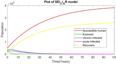
From Figure 2 we see that all compartments accept susceptible and recovery converges to zero. In this case the
value of ! 0.128 which is 1. This shows all comportment converges to disease free equilibrium point. Therefore, this provides absence of disease in the population and the disease dies out.
Figure 2. Numerical simulation of model for ! 0.128.
Figure 3. Numerical simulation of model for ! 3.5887.
4.2. The Role of Vaccination on the Dynamics of the Disease
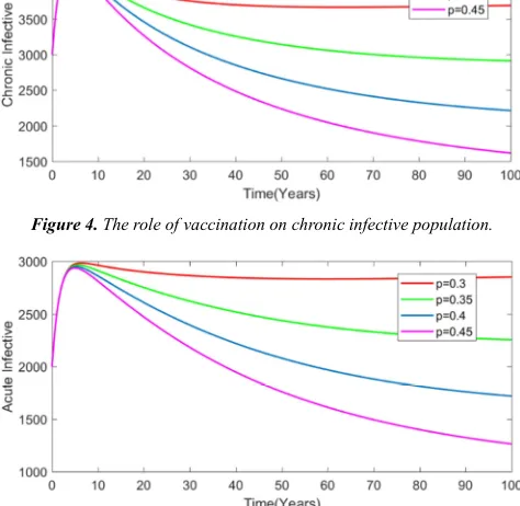
In Figure 4 it is observed that if the vaccination is increased then the chronic infective population is decreased accordingly.
Figure 4. The role of vaccination on chronic infective population.
Figure 5. The role of vaccination on acute infective population.
In Figure 5 it is observed that if the vaccination is increased then the acute infective population is decreased.
The simulation studies in Figures 4, 5 indicate that the increase in the vaccination rate results in the decrease of the infectious population sizes. Symbolically, the quantities and will decrease as increase. This simulation study indicates that the vaccination can play a great role to prevent the spread of hepatitis B virus disease.
4.3. The Role of Treatment Rate on Chronic Infective Population
Figure 6. The role of treatment rate on chronic infective population.
From Figure 6 it is observed that as the treatment rate is increased the chronic infective population size is decreased. This shows that the treatment of chronic infective population
has a great role in eliminating the hepatitis B disease. Thus, the public must be educated so that chronic infective people will take the medical treatment on time and thus leading to elimination of the disease.
4.4. The Effect of Transmission Rate on Infective Population
Figure 7. The effect of transmission rate on chronic infective.
From figure 7 we observe that as transmission rate increase then chronic infective population becomes increase. This shows one chronic infective person will produce averagely more than one infectious.
Figure 8. The effect of transmission rate on chronic infective.
From Figure 8 we observe that as transmission rate increase acute infective also increase. This shows one acute infective person will produce averagely more than one infectious.
Because if the transmission rate increase, then after some times the basic reproduction number is increase or become greater than 1 that is the disease persist in the population and infective populationbecomes increase.
4.5. The Effect of Sensitive Parameters on Basic Reproductive Number
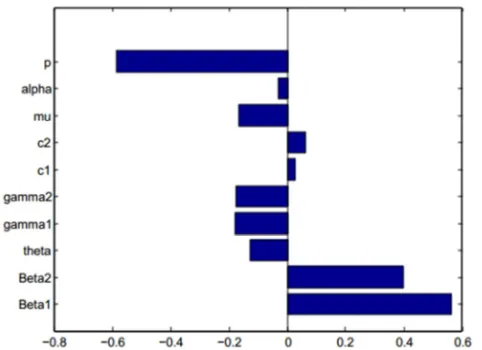
From Figure 9 it can be observed that some of the parameters are directly proportional to the basic reproduction number since they contribute for its growth while the remaining are inversely proportional since they contribute for the decay. The parameters , , , , have direct
proportionality with . In contrast, the
Figure 9. Effect of the sensitive parameters on the basic reproduction number.
5. Conclusions
In this study, the existing four –
compartmental model is modified and extended to a five compartmental model to describe the population dynamics with respect to HBV disease. The spread of HBV by considered with the inclusion of both vaccination and treatment rates. The present model is mathematically well-posed and biologically meaningful since the model variables are proved to be both positive and bounded.
Through the stability analysis it is shown that the disease free equilibrium point is locally and globally stable if < 1. This means that the transmission of disease is under control and because of this reason all individualswill survive. On the other hand, the disease frees equilibrium point is unstable if 1 which means that the disease invade or persist the population. However, the endemic equilibrium point is locally stable if 1.
The numerical simulation study shows that if the transmission rate increases then both chronic and acute infective populations will also increase. Additionally, if the vaccination rates increases then the infective population will decrease. Furthermore, if the treatment rate is increased then the chronic infective will decrease. Therefore, in order to prevent the spread of hepatitis B virus it is advised to (i) increase the vaccination to newly born babies and (ii) increase medical treatment to chronic infective population.
Thus, the mathematical analysis and simulation results of this study indicate thatin preventing the spread of hepatitis B virus both the vaccination and treatment play a great positive
role.
References
[1] U. S. Department of Health and Human Services, center for Disease control and prevention, 2016.
[2] World Health Organization, Hepatitis B virus: epidemiology and transmission risks, 2015.
[3] Tahir Khana, Gul Zamana and M., Ikhlaq Chohanb, The transmission dynamic and optimal control of acute and chronic hepatitis, Journal of Biological Dynamics, 11: 1, 172
− 189, 2017.
[4] Saher, F., Rahman, K., Quresh, J. A., Irshad, M. and Iqbal, H. M., Investigation of an Inflammatory Viral Disease HBV in Cardiac Patients through Polymerase Chain Reaction, Advances in Bioscience and Biotechnology, 3, 417 −422. http: //dx.doi.org/10.4236/abb.2012.324059., (2012).
[5] Hindia Nurhasen, The Transmission Dynamics and Optimal Control of Hepatitis B in Ethiopia Using SVEIRS Model, Addis Ababa University, October, 12, 2017.
[6] Moneim I. A. Al-Ahmed M. and Mosa G. A., Stochastic and Monte Carlo Simulation for the Spread of the Hepatitis B, Australian Journal of Basic and Applied Sciences, (2009) 3,
1607 − 1615. [7] Saint Paul, Minnesota,
www.immunize.org.www.vaccineinformation.org www.immunize.org/catg.d/p4205.pdf 651 − 647 − 9009. [8] I. A. Moneim, H. A. Khalil, Modeling and Simulation of the
Spread of HBV Disease with Infectious Latent, Applied Mathematics, 2015, 6, 745−753.
[9] Sacrifice Nana-Kyere, Joseph Ackora-Prah, Eric Okyere, Seth Marmah, Tuah Afram, Hepatitis B Optimal Control Model with Vertical Transmission Applied Mathematics, Applied Mathematics 7 (1): 5 − 13, 2017.
[10] WHO, Hepatitis B Factsheet, (2001).
[11] Tadele Tesfa Tegegne, Purnachandra Rao Koya and Temesgen Tibebu Mekonnen, Modeling and Simulation study of the Dynamics of HIV/AIDS due to Heterosexual and Vertical Transmissions, Hawassa, ETHIOPIA, 20015.
[12] Molalegn Ayana, Modeling the Impact of Infective Immigrants on the Dynamics and Spread of Zika virus, Hawassa, Ethiopia June, 2017.