level-of-detail adaptation of navigation services
Jelle De Bock
∗, Steven Verstockt
Ghent University - imec, Internet Technology and Data Science Lab, AA Tower, Technologiepark 122, B-9052 Gent, Belgium, [jelle.debock, steven.verstockt]@ugent.be
* Corresponding Author
Abstract: SmarterRoutes aims to improve navigational services and make them more dynamic and personalised by data-driven and environmentally-aware road scene complexity estimation. SmarterRoutes divides complexity into two subtypes: perceived and descriptive complexity. In the SmarterRoutes architecture, the overall road scene complexity is indicated by combining and merging parameters from both types of complexity. Descriptive complexity is derived from geospatial data sources, traffic data and sensor analysis. The architecture is currently using OpenStreetMap (OSM) tag analysis, Meten-Vlaanderen (MIV) derived traffic info and the Alaro weather model of the Royal Meteorological In-stitute of Belgium (RMI) as descriptive complexity indicators. For the perceived complexity an image based complexity estimation mechanism is presented. This image based Densenet Convolutional Neural Network (CNN) uses Street View images as input and was pretrained on buildings with Bag-of-Words and Structure-from-motion features. The model calculates an image descriptor allowing comparison of images by calculation of the Euclidean distances between descrip-tors. SmarterRoutes extends this model by additional hand-labelled rankings of road scene images to predict visual road complexity. The reuse of an existing pretrained model with an additional ranking mechanism produces results correspond-ing with subjective assessments of end-users. Finally, the global complexity mechanism combines the aforementioned sub-mechanisms and produces a service which should facilitate user-centred context-aware navigation by intelligent data selection and/or omission based on SmarterRoutes’ complexity input.
Keywords:data mining, machine learning, trajectory analysis (dealing with quality and uncertainty), traffic analysis, web and real-time applications
1. Introduction
Asroadsgetmorebusyandourlivingareasmoredensely
populated,driving hasbecomechallenging, especiallyin
cognitivelydemandingcircumstancessuchascomplex
junc-tionsor trafficcongestion. In thosehighly critical
situa-tionsextrahelpwouldbehighlybeneficialforaroaduser.
AdvancedDriverAssistanceSystems(ADAS)isthe
col-lectivetermtodescribethesesupportivetechnologies((EC),
2016)(Researchetal.,2002).Brakingsupport,lane
detec-tion, parking aidand emergencycalls are justa handful
of the numerouseffortsthat have beenmade toimprove
driving safety. However, thesestate-of-the-artassistance
featuresareusuallydesignedfortheaveragedriver. There
islittleornoinputfromtheuser-meaningitisgenerally
onlyrelying onsensorsof thevehicle tomakedecisions
(Hasenj¨ager and Wersing, 2017). Recently, somemajor
contributionstowardsuser-centreddata-drivennavigation
assistancehavebeenmade. Asanexample,Okamotoand
Tsiotras(OkamotoandTsiotras,2019)aredemonstrating
thatadditionaldatamightimproveADASimplementations
byadata-drivensteering wheeltorquepredictionmodel.
Combinedwithdriverbehaviourprofiling(Ferreiraetal.,
2017)suchamodelcouldhelpdrivingassistanceplatforms
betterpredictandpreventpossiblecrashesbasedonadriver’s
steeringcombinedwithknowledgeabouthis/herbehaviour
profile.
1.1 Complexitydrivenroutesuggestion
Along with the aforementionedassisting technologiesan
optimalroutewithappropriate, well-timednavigation
in-structionscanalsocontributetotheuser-centred
context-awaredrivingexperience. Giannopolousetal. discovered
forinstancethatdriverageandspatialabilitieshavea
con-siderable influenceon the desired timingsof the
naviga-tioninstructions(Giannopoulosetal.,2017).Sladewskiet
al.(Sladewskietal.,2017)implementedarouteplanning
layoutbasedonweightsoriginatingfromrankingtheroad
turns andtheir accompanied complexity. Thisis agreat
exampleoflessapparent characteristicswhichmake
nav-igationchallenging. In complexurban situations, drivers
(andespeciallyolderorinexperiencedones(Giannopoulos
etal.,2017))mightnotwantthefastestbutsafestor
eas-iestroute. Duchhametal. ((DuckhamandKulik,2003))
implementedsucharoutingalgorithmandfavouredroutes
withless complex manoeuvres overtheabsolute shortest
path. They also found that an easier routefrom A toB
wasonaverage16%longerthantheircorresponding
short-est path. Similar approaches are the algorithm of Krisp
andKeler(KrispandKeler,2015),estimatingcomplexity
basedonthenumberofnearbynodesdetectedinOSM,and
the Least AngleStrategy of Hochmair(Hochmair, 2000)
whichprefers roads withthe least deviationfrom the
1.2 User driving preferences
Another contributing factor towards user-centred context-adaptive navigation is the inclusion of user preferences and customisation. (Michon and Denis, 2001) performed a user study to get an idea of how the users would formulate nav-igation instructions after they were shown the way from a starting point to a destination in Paris. They found that the test persons often fell back on landmarks (e.g. objects or buildings standing out of the environment) when manoeu-vres became more difficult and complex. Various efforts have been made to elaborate landmark based orientation in navigation instructions. Richter and Klippel (Richter and Klippel, 2005) implemented a solution which started from basic and abstract routing directions that were then pro-jected on the actual environmental situation. The finding that users prefer landmark based navigation when com-plexity increases can be incorporated in SmarterRoutes’ implementation. The utilisation of meta-information from geospatial data sources (e.g. does a given intersection have traffic lights or is there a bus stop nearby) serves as an input for complexity estimation during navigation.
The overall advancement of technology and the availabil-ity of extensive (real-time) data introduces the need for data management as navigation and driving can become very challenging with an overload of data at inappropriate moments. Driving and navigating can be sometimes very challenging. A mixture of bad weather conditions, busy traffic and complex driving environments combined with data-overload and very complex driving instructions might cause dangerous situations for the driver (Rolison et al., 2018). To prevent such situations from happening, data-filtering and the provision of appropriate, well-timed in-structions should be implemented. This paper tries to con-tribute to the risk-assessment and data-filtering process by the proposal of a road-scene complexity judgement model based on the combination of geospatial, sensor and image data.
1.3 What is complexity?
Before the components of our complexity system are intro-duced, we should first define what a complex system actu-ally is. The exact definition of complexity has evolved over the years. In the early days, the Latin word “complexus” literally meant “weaving things together” (Schlindwein and Ison, 2004). Ottino (Ottino, 2003) came with a definition for complex systems. They concluded that a system can be considered complex if a lot of individual components and interactions exist. As a lot of things happen simulta-neously and are dependent of each other, it is acceptable to consider the road network and the accompanied traffic as a complex system. The different types of roads with all its road furniture and the interactions of drivers with each other and with the road infrastructure are perfect examples of elements which define the overall complexity of a road scene. Schlindwein and Ison concluded that a major def-inition of complexity can be best described by classifying the possible assessments of them in one of the two sub-categories; descriptive or perceived complexity. The for-mer, is the category in which quantitative measurements of complexity can be placed. In our road based context we can sum up a number of examples such as the number of cars on the road, the distance between them or the num-ber of speed bumps. The latter, perceived complexity, is
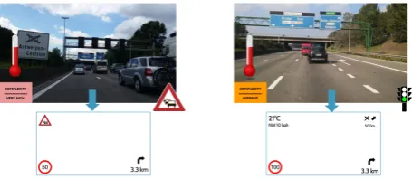
Figure 1. A visualisation of context aware data display whilst driving. Show less information when their is con-gestion.
the group which tries to quantify the perception of an ob-server. In our situation, this can be the thoughts of a driver whilst riding a certain road segment (e.g. this looks dan-gerous or this sector is badly illuminated or I can barely see the road).
A distinct complexity indication might on its turn serve as ultimate input for a smart navigation implementation. In the following subsections we discus the aforemetioned building blocks of the complexity mechanism in further de-tail.
2. The complexity mechanism
2.1 Level-of-detail driven data management
pro-vides just enough information to conveniently orient them-selves. In a user-centred navigational approach this choice should really be up to the users themselves. A parametric dashboard architecture which offers a predefined collec-tion of data fields and services based on the type of user might be a good design to fulfil this important aspect of user-driven navigation.
Nonetheless, Cellario (Cellario, 2001) pointed out that a huge amount of data might cause information overload dur-ing drivdur-ing. Research performed by Morris et al. (Morris et al., 2015) showed that distractions of as little as 2 seconds considerably increase the risk for an accident. The US department of Transportation also made considerable ef-forts in this field of study. They concluded that information should be checked against the following criteria: informa-tion type; priority and complexity; trip status and driving load; and the driver profile (Hulse et al., 1998). Although the latter two criteria are undeniably very important to the safety of an intelligent navigation system we will mainly focus on the former aspect of data filtering. The added dimension of data and distraction management introduces a supplementary use case for the context-aware complex-ity indication mechanism. In the following subsections, a mechanism to estimate environmental road scene com-plexity based on image, geospatial and sensor data will be discussed.
2.2 Scoring an environment’s complexity
Generally, humans are capable to visually judge the im-mediate risk of a certain road situation. This is what we previously called the perceived complexity of an individ-ual. In sheer contrast, traffic accident studies show that the major part of incidents are caused by human mistakes (Rolison et al., 2018). A human’s judgement is the result of the combination from input of our senses with our gath-ered background knowledge. The eyes take a snapshot of the environment and the human brain tries to link this snap-shot with previously encountered situations. Background knowledge about the type of environment ultimately pro-vides us with an idea of the road scene’s complexity. To mimic this natural behaviour the proposed complexity mea-surement mechanism uses transfer learning on Convolu-tional Neural Networks (CNNs) with human judgements of visually perceived risk of a road scene as training labels. A Convolutional Neural Network is a deep neural network which is especially suitable for image input. Image input is processed by a variety of matrix operations which are reducing the individual pixels to a feature matrix. The ex-act feature matrix is the result of training the model with training data for a specific use case (e.g. road type classifi-cation). For readers who want a more in-depth introduction into convolutional neural networks we refer to the work of O’Shea and Nash (O’Shea and Nash, 2015).
Visual complexity score: Convolutional Neural Net Im-age Retrieval (CIR) As mentioned, increasing road com-plexity clearly imposes the need for context-adaptive nav-igation and driving assistance. The first component of the complexity estimation mechanism is computer-aided vi-sual road scene complexity estimation. In the next para-graph we will introduce such an implementation which emulates the human’s visual road scene perception. The suggested implementation uses the proposed framework of Radenovi´c et al. (Radenovi´c et al., 2018). Their solution
excels in finding similarity among images and achieves this by careful selection of descriptor features. Positive matches were detected in large image data sets based on a combination of Bag-of-Words (BoW) and Structure-from-Motion techniques. As negative matches the closest neg-ative image and its k-nearest neighbours are selected (a match is marked as negative by additional 3D reconstruc-tion methods verifying that the match isn’t just showing the object from another point of view). When the tuples (image, best positive match, closest negative matches) are calculated for a training dataset a Convolutional Neural Network can be fine-tuned to minimise positive matching distances and maximising the negative matching ones (see Fig. 2 for the schematic overview of this approach). Fig. 3 illustrates that the model is very capable at finding a visu-ally very similar image in its collection of labelled training data.
Figure 2. Radenovi´c et al. image matching architecture
Figure 3. Best match provided by the model providing it with ”Original image” as an input.
images (18) were hand labelled. Rankings accompanied by their image paths are stored in a separate csv file. Like-wise, image descriptors are calculated using the pretrained model of Radenovi´c et al. (Radenovi´c et al., 2018) and are stored in .h5 files (Hierarchical Data Format). Road scene complexity can now be estimated by calculating the descriptor of a new/unseen street scene image and by com-paring them with the descriptors in the indexed h5 file con-sisting of the training images. Image similarity is defined as the euclidean distance between their descriptors. Eq.1 and Eq. 2 calculate the best and second best match for an
image query (IQ). When the best (Ibest) and the second
best match (I2ndbest) is known a weighted final score (Eq.
3) can be determined. The exact weights are currently set
to 34 and 14. Further and thorough evaluation is needed to
fine-tune and verify the values for the weights.
Ibest= min I0...In
[dist(Ii, IQ)] (1)
I2ndbest= min
I0...In\Ibest
[dist(Ii, IQ)] (2)
W =w1∗Wbest+w2∗W2ndbest (3)
With:
Ii training image i (i≤0< n))
IQ query image
dist(Ii, Q) euclidean distance between descriptors
training imageiand query image
W total and final weight ofIQ
w1 weight of best match
w2 weight of second best match
Wbest score of best matching training image
(from CSV)
W2ndbest score of second best matching training
image (from csv)
Figure 4. Step by step schematic overview of the image based complexity ranking mechanism
Model and ranking mechanism evaluation In the pre-vious paragraph the image-based ranking model was intro-duced. The approach looks promising as the real power lies in the flexibility, relative simplicity and ease of use. The biggest contributor to its overall ranking potential is the adoption of a well established pretrained model tailored for recognising similarity in 3D objects (buildings or road scenes). When this is combined with an additional ing (and lookup) mechanism, a basic but functional rank-ing mechanism is obtained. When we would have opted to retrain an entire model for the image-based complexity judgement task we should need a lot of labelled training
data (M. Foody et al., 1995), which unfortunately isn’t yet the case, but is an aspect we are actively working on. The re-use of an existing CNN-based similarity model, com-bined with an initial collection of road scene images which are accompanied by human labelled rankings, already pro-vides us with a basic, but usable model. Initial user tests show that generated complexity scores are corresponding with subjective evaluations of the testers.
Additionally, to verify this first iteration of the CNN based complexity gauging mechanism, 20 hand labelled images were used to validate the model. As previously discussed, the model used to determine perceived complexity is look-ing for similarity in the images to find the best match in the dataset (images with calculated CNN descriptors and the human-labelled complexity). The bigger and more univer-sal this dataset is, the bigger the chance of finding a road scene with similarly looking characteristics (e.g. bridges, zebra crossings). With this consideration in mind, the
ini-tial model’s achieved mean square error (MSE) of2.92is
a promising starting point for the following versions with more and extended geographically covering human-labelled street scene images.
Geospatial and sensor complexity analysis of a road scene The CNN-based model and ranking system em-ulates the visually perceived road scene safety. As men-tioned in the introduction, human perceived complexity isn’t always an accurate gauge for the actual complexity. The big number of road accidents which are occurring due to human error are a perfect example for this fact. When we want to obtain a complexity model that minimises the potential danger of human (mis)perception, we should also include descriptive complexity indicators into our complex-ity mechanism.
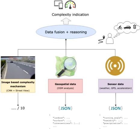
Figure 5. A visual representation of the complexity esti-mation model with all of its sub ranking mechanisms
the road situation is perceived by a road user. In a next step, the initial value can be checked against or further fine-tuned by the descriptive complexity indicators of the archi-tecture. Currently we have implemented geospatial analy-sis (Fig. 5) using OpenStreetMap as its data source. This mechanism is providing us with meta-information about the road which the driver is currently using. Table 1 shows the geospatial information which is obtained for our com-plexity mechanism by an example. The properties are al-lowing categorisation of the environment based on land-use (e.g. grassland, woodland and urban) and road type (e.g. highway, primary, secondary) during the fusioning and reasoning stage (Fig. 5) . The other currently imple-mented descriptive measures of complexity are traffic and weather analysis.
This modular approach facilitates additional inclusion of sensor data to adapt the complexity scoring to a specific use case based on additional and carefully selected environ-mental and peripheral input (e.g. extra inclusion of turn-ing angle or driver stress level). Furthermore, as more and more people tend to carry a smartphone, active research around additional useful sensor data should definitely be considered. An example of a possibly useful sensor is the accelerometer which is standard equipment for most ev-eryday smartphones. Logging acceleration and monitoring changes over time might provide valuable contributions to-wards overall complexity estimation. Zang et al. (Zang et al., 2018) proposed a method for road surface roughness estimation using a mobile application. Their work is ba-sically showing the possibility to get road surface insights from smartphone acceleration sensors. For certain trans-port modes (e.g. motor riders or cyclists) accelerometer data might also provide an approximate leaning angle dur-ing turns (Ldur-ingesan and Rajesh, 2018). When both surface knowledge and tilt angles are combined a general idea of how “sporty” a bike rider is taking turns and provide them with a warning if a certain leaning angle was too extreme for a given type of road.
Another interesting input source might be real-time im-agery coming from action or dash cameras. This bypasses the use of Street View based road scene images, which aren’t always optimally representing the current road sit-uation (e.g. different time of the day, road works). Ad-ditionally, together with the guaranty of real-time footage which can be used for more accurate image based street scene complexity, more profound insights in the environ-ment might be obtained as well. Some examples of possi-ble insights are weather situation (clouded or clear sky or even temperature (Chu et al., 2018)) or image based road surface categorisation (Slavkovikj et al., 2014).
2.3 The influence of user characteristics on complex-ity
The previously introduced complexity mechanisms were all based on the road environment and its related context. The characteristics of the end-user are another equally im-portant factor which should also be considered in a context-aware LoD-management platform. As mentioned in the introduction of this paper (section 1), several interesting studies around a user’s navigational behaviour do exist. Two important user specific characteristics are their age and their general sense of direction. Combination of both characteristics can result in various driver profiles which
can be linked to specific rules on how they behave at a cer-tain complexity level. For instance, when a driver is pro-filed as “a novice driver with mediocre geospatial capabili-ties, these rules might result in the omission of certain data in favour of more thorough route guidance during complex driving situations.
Finally, a global complexity indication mechanism can be compiled using the various sources of geospatial and sen-sor data combined with knowledge about the type of driver. With the help of this indication, a data-driven navigation service should now be able to make a well considered de-cision about which information to omit/display and how exactly to display the necessary information, based on the complexity ranking and the provided user preferences.
3. Evaluation
In the previous section the various components of the com-plexity framework have been discussed in detail. A follow-ing step consisted of testfollow-ing the introduced mechanisms against some real-life scenarios to check if the indicators are corresponding with these scenarios.
Figure 6. R1, Antwerp, relatively quiet traffic, image based complexity 1.5/10 (i.e. low complexity)
Figure 7. R1, Antwerp, congested traffic, image based complexity 8.75/10 (i.e. high complexity)
Image based complexity 5.25(/10)
General OSM analysis
Closest OSM way id 130795868
Road type tertiary
Road surface unknown
Land Use unknown
Maximum speed unknown
Closest intersection
Bearing angle 263
Distance from location 0.07km
Latitude 51.1740211
Longitude 3.9377042
n-type 3
Traffic info
distance from location 2.77km
Latitude 51.19891697
Longitude 3.93597038
Road description Complex nr 12 Moerbeke
Road type driving lane
Speed difference 19
Speed cars 72
Road occupation 1
Weather info
Precipitation 0.00002m
Wind angle 63
Wind direction North
Wind speed 3.20m/s
Temperature 9.95◦C
Table 1. Complexity analysis results for rural town centre of Fig. 8
our decision to split complexity in a perceived and descrip-tive sub-component. The time- and context-dependency on perceived complexity could be bypassed by the use of ac-tion or dash cams as they would provide the model with a real time snapshot of the environment. As an additional bonus, they also avoid the process of downloading and pro-cessing Street View footage. Experiments have shown that this exact process takes the longest time in the entire com-plexity ranking mechanism (5.42 seconds were needed to download and process the Street View image, the entire complexity indication process took 9.75 seconds).
Figure 8. Complexity analysis for a rural town centre, showing the various mechanism parameters in table 1. Fur-ther reasoning about the parameters indicate average com-plexity
The data selection and processing of potential
complex-ity analysis mechanisms was realised in correspondence with SmarterRoutes’ general concepts and principles about modularity. Extra components can be added as needed and the subsequent reasoning and unification of the selected mechanisms ideally happen on a user(group) level.
To demonstrate and verify the perceived complexity CNN model, we implemented a basic set of descriptive complex-ity parameters to suit a broad group of users’ needs. Cur-rently, geospatial analysis is performed by OSM way tag analysis supplying maximum speed, land use, road type and basic intersection information. Sensor based analytics are obtained from the Alaro weather model from the
Bel-gian Meteorological Institute (RMI)1 providing the
com-plexity mechanism with precipitation, temperature and wind condition. Traffic information was obtained by periodi-cally polling the data resulting from the governmental
ini-tiative “Meten in Vlaanderen (MIV)”2which analyses the
traffic statuses of Belgium’s major roads and is providing the model with real-time vehicle speeds, road occupation and speed difference for a certain location.
As a showcase for the various mechanisms we show the analysis for a road scene of a Flemish village centre. Fig-ure 8 shows the full complexity analysis for the centre of Moerbeke-Waas, Flanders. As indicated the perceived im-age based complexity mechanism indicates averim-age com-plexity (5.25/10). As shown under “Closest intersection” (Table 1) and also visible on the map in Figure 8 a 3-way intersection is nearing. This fact should also be considered in the overall complexity estimation. Traffic info is irrel-evant for this exact location as the closest measurement point is more than 2km away. Additionally, the geospatial (tertiary road) and sensor based analysis (i.e. good weather and relatively low wind speed) indicate that the road scene circumstances are relatively safe. The final recommenda-tion coming out of the model would be “average complex-ity, intersection coming up”.
As mentioned the image based complexity mechanism was using a minimal amount of training data and the initial
model is giving a MSE of2.92on a verification set of 20
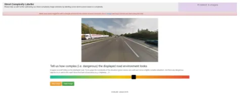
images. We are currently gathering more training data, to get a bigger and geographically broader dataset. For this additional data gathering a number of A to B routes were calculated and Street View footage was obtained for these routes. A total of 6 routes (see Fig. 9), spread across the Flanders region (Belgium), resulted in a total of 2245 im-ages which will be hand labelled by test users using an in-house web-based labelling tool (see Fig. 10).
Nevertheless, as the model might become more accurate by providing it with more training data, perceived complexity will still have several shortcomings. First, an important consideration is the fact that Street View images are just snapshots of the environment. This footage can be out-dated or even unavailable for certain regions. Another im-portant consideration is that complexity can change through-out the day. For instance, a highway will look more com-plex when a lot of vehicles are on the Street View image then it would do when traffic was entirely quiet.
1https://opendata.meteo.be/geonetwork/srv/eng/
catalog.search#/metadata/RMI_DATASET_ALARO 2
Figure 9. Geographical spread of the routes used to gather additional training data.
Figure 10. The user-friendly web interface to conveniently label the route’s (see Fig. 9) Street View images.
4. Conclusion
The introduced SmarterRoutes complexity mechanism was implemented with end-user customisation and simplicity in mind. The human’s perceived complexity is replicated by a CNN-model with an additional ranking mechanism. In addition, geospatial and sensor based analysis provide descriptive complexity measurements which are fine-tuning or correcting the user perception about road complexity. Basic and straightforward fusion and reasoning has already been experimented with (e.g. primary roads are more plex as secondary or traffic congestion means high com-plexity), but additional, future work should be done to stream-line the process.
A big consideration is the fact that the whole mechanism is centred around data. The mechanism’s performance is highly dependant on the quality of the supplied data. As shown in Table 1, land use, road surface or maximum speed are often unknown as users haven’t yet contributed this
in-formation to the OSM database (seehttps://taginfo.
openstreetmap.orgfor an idea of the coverage for cer-tain OSM tags). Additional geospatial datasets or data aug-mentation methods could be used to get more coverage (for instance, the work of Slavkovikj et al. (Slavkovikj et al., 2014) and could be considered in future iterations of the geospatial complexity mechanism).
Additionally, as we try to focus the whole complexity level-of-detail aware navigation and data-management around an individual the need for user studies arise. As previ-ously mentioned, the suggested image based complexity indication component would certainly benefit from addi-tional hand-labelled Street View images. When more la-belled test and training Street View data is used in our model, the MSE for the visual complexity model could be further reduced. Another direct benefit of user stud-ies would be the impact on the perceived complexity by
using different image sources. It would be very interest-ing to present the user the same road scene both as a Street View capture and a action cam image. This would poten-tially give further insights in the influence of weather situa-tion, season, time of day or other nuances on the perceived complexity. Combined with knowledge of traffic (and ac-cidents) experts we could possibly gain also more insights under which circumstances drivers are more likely to miss-estimate complexity.
References
Cellario, M., 2001. Human-centered intelligent vehicles:
Toward multimodal interface integration. IEEE intelligent
systems16(4), pp. 78–81.
Chu, W., Ho, K. and Borji, A., 2018. Visual weather
tem-perature prediction. CoRR.
Duckham, M. and Kulik, L., 2003. “simplest” paths: Au-tomated route selection for navigation. In: W. Kuhn, M. F.
Worboys and S. Timpf (eds),Spatial Information Theory.
Foundations of Geographic Information Science, Springer Berlin Heidelberg, Berlin, Heidelberg, pp. 169–185. (EC), E. R. S. O., 2016. Advanced driver assistance sys-tems summary.
Ferreira, J´unior, J., Carvalho, E., Ferreira, B. V., de Souza, C., Suhara, Y., Pentland, A. and Pessin, G., 2017. Driver behavior profiling: An investigation with different
smart-phone sensors and machine learning. PLOS ONE12(4),
pp. 1–16.
Giannopoulos, I., Jonietz, D., Raubal, M., Sarlas, G. and
St¨ahli, L., 2017. Timing of Pedestrian Navigation
In-structions. In: E. Clementini, M. Donnelly, M. Yuan,
C. Kray, P. Fogliaroni and A. Ballatore (eds),13th
Interna-tional Conference on Spatial Information Theory (COSIT 2017), Leibniz International Proceedings in Informatics (LIPIcs), Vol. 86, Schloss Dagstuhl–Leibniz-Zentrum fuer Informatik, Dagstuhl, Germany, pp. 16:1–16:13.
Hasenj¨ager, M. and Wersing, H., 2017. Personalization in advanced driver assistance systems and autonomous
vehi-cles: A review. In: 2017 IEEE 20th International
Confer-ence on Intelligent Transportation Systems (ITSC), pp. 1– 7.
Hochmair, H., 2000. ”least angle” heuristic: Consequences of errors during navigation. pp. 282–285.
Hulse, M. C., Dingus, T. A., Mollenhauer, M. A., Liu, Y., Jahns, S. K. and Brown, T., 1998. Development of hu-man factors guidelines for advanced traveler information systems and commercial vehicle operations : identification of the strengths and weaknesses of alternative information display formats. Research Paper.
Krisp, J. M. and Keler, A., 2015. Car navigation –
comput-ing routes that avoid complicated crosscomput-ings. Int. J. Geogr.
Inf. Sci.29(11), pp. 1988–2000.
Lingesan, B. and Rajesh, R., 2018. Tilt angle detector us-ing 3-axis accelerometer.
M. Foody, G., Mcculloch, M. and Yates, W., 1995. The effect of training set size and composition on artificial
neu-ral network classification.International Journal of Remote
Sensing - INT J REMOTE SENS16, pp. 1707–1723. Michon, P.-E. and Denis, M., 2001. When and why are vi-sual landmarks used in giving directions? In: D. R.
Mon-tello (ed.), Spatial Information Theory, Springer Berlin
Heidelberg, Berlin, Heidelberg, pp. 292–305.
Naik, N., Philipoom, J., Raskar, R. and Hidalgo, C., 2014. Streetscore – predicting the perceived safety of one
mil-lion streetscapes. In:2014 IEEE Conference on Computer
Vision and Pattern Recognition Workshops, pp. 793–799. Okamoto, K. and Tsiotras, P., 2019. Data-driven human driver lateral control models for developing haptic-shared
control advanced driver assist systems. Robotics and
Au-tonomous Systems114, pp. 155 – 171.
O’Shea, K. and Nash, R., 2015. An introduction to
convo-lutional neural networks.CoRR.
Ottino, J. M., 2003. Complex systems. AIChE Journal
49(2), pp. 292–299.
Radenovi´c, F., Tolias, G. and Chum, O., 2018. Fine-tuning
CNN image retrieval with no human annotation.TPAMI.
Research, T., Monitoring, I. and (TRIMIS), I. S., 2002. Action for advanced driver assistance and vehicle control systems implementation, standardisation, optimum use of the road network and safety (final report).
Richter, K.-F. and Klippel, A., 2005. A model for
context-specific route directions. In: C. Freksa, M. Knauff,
B. Krieg-Br¨uckner, B. Nebel and T. Barkowsky (eds),
Spa-tial Cognition IV. Reasoning, Action, Interaction, Springer Berlin Heidelberg, Berlin, Heidelberg, pp. 58–78.
Rolison, J. J., Regev, S., Moutari, S. and Feeney, A., 2018. What are the factors that contribute to road accidents? an assessment of law enforcement views, ordinary drivers’
opinions, and road accident records. Accident Analysis
Prevention115, pp. 11 – 24.
Schlindwein, S. L. and Ison, R., 2004. Human
know-ing and perceived complexity: implications for systems
practice. Emergence: Complexity and Organization6(3),
pp. 27–32.
Sladewski, R., Keler, A. and Divanis, A., 2017. Computing the least complex path for vehicle drivers based on
clas-sified intersections. In: Proceedings of the AGILE 2017
conference on Geographic Information Science.
Slavkovikj, V., Verstockt, S., De Neve, W., Van Hoecke, S. and Van de Walle, R., 2014. Image-based road type
classi-fication. In:International Conference on Pattern
Recogni-tion, pp. 2359–2364.
Zang, K., Shen, J., Huang, H., Wan, M. and Shi, J., 2018. Assessing and mapping of road surface roughness based on gps and accelerometer sensors on bicycle-mounted