Transfer
Encoding Decoding
Sender Receiver
System
Patric Hindenberger
*, Volker SchwiegerInstitute of Engineering Geodesy, University of Stuttgart, Germany, [firstname.lastname]@iigs.uni-stuttgart.de
* Corresponding author
Abstract: Location Referencing is a well-known methodology to transfer geoobjects from one digital map to another and typically used to share traffic information. Here, especially the dynamic methods play a major role, as they are developed to transfer Location References between different maps in such cases where no common databases and/or common structures are available. The key issue in dynamic Location Referencing is to find the correct geoobject in the target map which corresponds to the geoobject in the source map. So far, in nearly all methods a deterministic algorithm is implemented to perform this. Given the fact that geodata as well as the matching procedure for geodata has some uncertainty, it is obvious to research uncertainty-based algorithms. This paper presents a probability-based decision system by formulating the decision algorithm/functions and evaluating them. The evaluation is done with real traffic information and benchmarked against a deterministic decision system.
Keywords: dynamic location referencing, digital maps, probability theory, decision system
1.
Introduction
For location-based services (LBS), digital maps are of crucial importance and are often provided in different versions. In the context of the transfer of geoobjects (locations) between two digital maps, the term Location Reference (LR) was introduced. Following various definitions for a Location Reference (Hackeloeer, 2016; Lv et al., 2008; Schützle, 2016; Wartenberg, 2007; Wevers, 2000), a Location Reference can be understood as a map-independent description or identification of a digital map based geoobject. The description itself is carried out by means of concrete attributes, which are derived from the well-known attribute categories for general geodata (de Lange, 2013; Devogele et al., 1996; Hagedorn, 2007; Lutz et al., 2009; Ma et al., 2010; Streit, 1996) and can be summarized and grouped as follows (Hindenberger and Schwieger, 2018):
• Geometrical attributes like coordinates/ bearing; • Topological attributes like node valence/degree; • Syntactical (or toponymical) attributes like the
name of an object;
• Semantical (or thematical) attributes like physical appearance of an object or hierarchy in road network.
As geoobjects in general (de Lange, 2013), a LR can consist in planar case of points, lines and areas (Schützle, 2016) and cover typically use cases such as traffic or road information (Hackeloeer, 2016; Wevers and Hendriks, 2006). The umbrella term Location Referencing refers to a summary of all methods and techniques for transferring a LR (Wartenberg 2007; Schützle 2016) and represents a
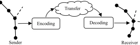
concrete variant of general georeferencing (Hackeloeer, 2016). The specific method is typically called Location Referencing Method (LRM) and used in a Location Referencing System (LRS) (Kenley and Harfield, 2018). The process (Location Referencing Process) within the Location Referencing System is one-dimensional without any iteration and typically the sender (source) and receiver (target) systems are distributed and separated. Svensk and Wikström (2013) and Schützle (2016) split the process in three steps: firstly with encoding the LR for a given geoobject on the side of the sender (i.e. the LR is generated in a defined interface format), secondly the transfer itself between sender and receiver system, and thirdly the decoding on the receiver side which means primarily performing the algorithm to find and detect the correct or the most likely geoobject for the transferred LR in the receiver system.
Figure 1. Process of Location Referencing (according to Svensk and Wikström (2013))
Samal et al., 2004; Stigmar, 2005). Hence, the use of a method to handle such uncertainty by concepts like probability theory is appropriate. However, such a method has just been used in one known LRM (TPEG2-ULR with Markov Chain published in Schramm et al. (2012)), so this makes it interesting to do some additional research and investigations.
Based on previous works published in Hindenberger and Schwieger (2018), this paper presents a probability-based decision system for LRS and is structured as follows: In Section 2 the mathematical principles in the context of the approach are given. Sections 3 and 4 describe the specific decision functions and underlying probability distributions. This is followed by the experimental evaluations in Section 5 and the paper closes with a conclusion given in Section 6.
2.
Mathematical principles
In this approach, the values are seen as random variables. So, in this section the relevant mathematical principles and methods are introduced in the following and used later in Sections 3 and 4.
2.1 Probability theory
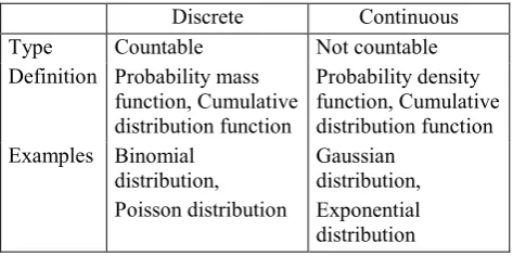
Probability is a measure of the occurrence of a random variable (Eckey et al., 2005). Here, the random variables are differentiated by discrete or continuous (Bosch, 1986) as shown in Table 1.
Table 1. Discrete and continuous random variables Discrete Continuous Type Countable Not countable Definition Probability mass
function, Cumulative distribution function
Probability density function, Cumulative distribution function Examples Binomial
distribution, Poisson distribution
Gaussian distribution, Exponential distribution
In this paper, the exponential and binomial distributions are relevant in particular (compare Section 4.2).
In specific, the exponential distribution is defined as (Bronstein et al., 1993):
𝑓𝑓(𝑥𝑥) =�0, 𝑥𝑥𝜆𝜆𝑒𝑒−𝜆𝜆𝜆𝜆 𝑥𝑥 ≥< 00 , (1)
where 𝜆𝜆=1𝜇𝜇, 𝜇𝜇=𝑒𝑒𝑥𝑥𝑒𝑒𝑒𝑒𝑒𝑒𝑒𝑒𝑒𝑒𝑒𝑒 𝑣𝑣𝑣𝑣𝑣𝑣𝑣𝑣𝑒𝑒.
Furthermore, the binomial distribution is given by (Bronstein et al., 1993):
𝐵𝐵𝑝𝑝𝑛𝑛(𝑘𝑘) = �𝑛𝑛𝑘𝑘�𝑒𝑒𝑘𝑘(1− 𝑒𝑒)𝑛𝑛−𝑘𝑘 , (2)
where p= probability of single event, n= number of trials,
k= number of successes in n trials.
In case of unknown distribution type, the distribution and the underlying parameters need to be estimated (Table 2) by a random sample and finally checked by a “goodness of fit” test (e.g. Kolmogoroff-Smirnoff-Test) to identify the probability distribution.
Table 2. Estimation of distribution parameters (according to Hartung et al. (2009))
Binomial distribution Exponential distribution 𝑒𝑒̂=𝑛𝑛𝑘𝑘=𝑓𝑓𝑟𝑟 (3)
𝑓𝑓𝑟𝑟=𝑟𝑟𝑒𝑒𝑣𝑣.𝑓𝑓𝑟𝑟𝑒𝑒𝑓𝑓𝑣𝑣𝑒𝑒𝑓𝑓𝑒𝑒𝑓𝑓
𝜆𝜆=1𝜇𝜇=𝐸𝐸(1𝑋𝑋�)≈𝜆𝜆̅1 = 𝜆𝜆̂ (4)
𝑥𝑥̅=𝑚𝑚𝑒𝑒𝑣𝑣𝑓𝑓𝑜𝑜𝑓𝑓𝑟𝑟𝑣𝑣𝑓𝑓𝑒𝑒𝑜𝑜𝑚𝑚𝑠𝑠𝑣𝑣𝑚𝑚𝑒𝑒𝑣𝑣𝑒𝑒
By a Kolmogoroff-Smirnoff-Test, the test criterion 𝐷𝐷𝑚𝑚𝑚𝑚𝜆𝜆 is verified against a critical value 𝐷𝐷1−𝛼𝛼 which needs to be reduced in case of parameter estimation. This critical value 𝐷𝐷1−𝛼𝛼 is given for an exponential probability distribution with estimated parameter 𝜆𝜆 on significance
level α=0,05 and random sample size n>30 as (Hartung et
al., 2009):
𝐷𝐷1−∝=0,95=1,08
√𝑓𝑓 , 𝑓𝑓> 30 (5) 2.2 Deterministic and probability-based approaches Mathematical decision concepts can be distinguished into deterministic or uncertainty-based approaches. In the deterministic case, the values are uniquely determined, whereas in the case of uncertainty, the values base on random variables (stochastic, probability-based) or are fuzzy (Rommelfanger and Eickemeier, 2002).
Typically, deterministic values are described by analytical functions which are combined to a final power (or cost) function. This function will be maximized (or minimized) to get the final decision value (Dinkelbach, 1969). Stochastic values themselves are handled by the methods of probability theory. In case of multiple individual probabilities these are also combined. Here, it has be differentiated between stochastically independent and stochastically dependent probabilities. For independent probabilities, single probabilities 𝑒𝑒1, … ,𝑒𝑒𝑛𝑛 are multiplied (Equation 6) whereas for dependent probabilities, the „multiplication rule for conditional probabilities“ needs to be used (Hartung et al., 2009):
𝑒𝑒𝑟𝑟𝑟𝑟𝑟𝑟 = 𝑒𝑒1∗… ∗ 𝑒𝑒𝑛𝑛 (6)
Similar to the deterministic approach, the probability-based approach is an optimization task which means the maximum (or minimum) value will be used to make the final decision (Dinkelbach, 1969; Kromphardt et al., 1962).
3.
Deterministic and probability-based decision
functions
3.1 Definition of criteria
geospatial data sources, (Bruns and Egenhofer, 1996; Gösseln and Sester, 2004; Li and Goodchild, 2012; Rodriguez and Egenhofer, 2004; Volz and Walter, 2004) and play a major role in many applications such as spatial decision systems etc. (Schwering, 2008).
Following Hindenberger and Schwieger (2018), Table 3 shows the selected criteria (similarity measurements) with the focus on linear geoobjects (e.g. roads) described by the topological elements of nodes and edges.
Table 3. Criteria for probability-based decision system
Geometrical
• node distances between two nodes
• bearing differences between edges (line segments)
Topological
• Comparison of node valences/degrees
Syntactical
• Comparison of street names
Semantical
• Comparison of Functional Road Class (FRC)
• Comparison of Form of Way (FOW)
• Comparison of speed categories
• Comparison of one-way-attribute
As pointed out by Hindenberger and Schwieger (2018), the criteria listed result from the outcome of former works in this context, in which the criteria have been used and/or named as relevant (e.g. Schützle, 2016; Wartenberg, 2007).
3.2 Decision functions
In this paper, two groups of decision functions have been specified and formulated:
• Probability-based main function with full set of criteria as primary methodological outcome; • Probability-based and deterministic functions for
comparative calculation.
The latter is given by the fact, that absolute performance strongly depends on the aggregation of the specific test data and the definition of the performance indicator. So, it is necessary to perform such a comparative calculation by using a well-known deterministic approach. For this, the OpenLR-decision function (OpenLR demo implementation, described in Schützle (2016)) has been selected and adapted accordingly. In this, a reduced set of criteria by node distances, bearing differences and the comparison of FRC and FOW is used.
3.2.1 Probability-based functions
Using the full set of criteria, the probability-based main function is defined by Equation 7 following Equation 6 due to the stochastically independence of the criteria:
𝑒𝑒𝑟𝑟𝑟𝑟𝑟𝑟= 𝑒𝑒𝑛𝑛𝑛𝑛∗ 𝑒𝑒𝑏𝑏𝑛𝑛∗ 𝑒𝑒𝑣𝑣𝑚𝑚𝑣𝑣∗ 𝑒𝑒𝑟𝑟𝑠𝑠𝑟𝑟𝑟𝑟𝑟𝑟𝑠𝑠
∗ 𝑒𝑒𝑓𝑓𝑟𝑟𝑓𝑓∗ 𝑒𝑒𝑓𝑓𝑓𝑓𝑓𝑓∗ 𝑒𝑒𝑟𝑟𝑝𝑝𝑟𝑟𝑟𝑟𝑛𝑛 ∗ 𝑒𝑒𝑓𝑓𝑛𝑛𝑟𝑟𝑓𝑓𝑚𝑚𝑜𝑜 , (7)
where
Table 4. Variable names for probability-based decision function 𝑒𝑒𝑛𝑛𝑛𝑛= node distance,
𝑒𝑒𝑏𝑏𝑛𝑛= bearing difference, 𝑒𝑒𝑣𝑣𝑚𝑚𝑣𝑣= node valences, 𝑒𝑒𝑟𝑟𝑠𝑠𝑟𝑟𝑟𝑟𝑟𝑟𝑠𝑠= street name,
𝑒𝑒𝑓𝑓𝑟𝑟𝑓𝑓= functional road class, 𝑒𝑒𝑓𝑓𝑓𝑓𝑓𝑓= form of way, 𝑒𝑒𝑟𝑟𝑝𝑝𝑟𝑟𝑟𝑟𝑛𝑛= speed category, 𝑒𝑒𝑓𝑓𝑛𝑛𝑟𝑟𝑓𝑓𝑚𝑚𝑜𝑜: one-way-attribute. For the comparative calculation and the reduced set of criteria, the probability-based decision function is adapted accordingly by Equation 8:
𝑒𝑒𝑟𝑟𝑟𝑟𝑟𝑟′= 𝑒𝑒𝑛𝑛𝑛𝑛∗ 𝑒𝑒𝑏𝑏𝑛𝑛∗ 𝑒𝑒𝑓𝑓𝑟𝑟𝑓𝑓∗ 𝑒𝑒𝑓𝑓𝑓𝑓𝑓𝑓 (8)
The individual probability values are given by the probability distributions in Section 4.2.
3.2.2 Deterministic function
The OpenLR deterministic approach is specified as a deterministic power function given by Equation 9:
𝑅𝑅𝑂𝑂𝑝𝑝𝑟𝑟𝑛𝑛𝑂𝑂𝑂𝑂=𝑅𝑅𝑛𝑛𝑓𝑓𝑛𝑛𝑟𝑟∗ 𝑓𝑓𝑛𝑛+� 𝑅𝑅𝑠𝑠+ 𝑅𝑅𝑓𝑓𝑟𝑟𝑓𝑓+ 𝑅𝑅𝑓𝑓𝑓𝑓𝑓𝑓� ∗ 𝑓𝑓𝑟𝑟 , (9)
where 𝑅𝑅𝑛𝑛𝑓𝑓𝑛𝑛𝑟𝑟 = Rating factor for node distance, 𝑅𝑅𝑠𝑠 = Rating factor for bearing differences, 𝑅𝑅𝑓𝑓𝑟𝑟𝑓𝑓 = Rating factor for FRC,
𝑅𝑅𝑓𝑓𝑓𝑓𝑓𝑓 = Rating factor for FOW, 𝑓𝑓𝑛𝑛 ,𝑓𝑓𝑟𝑟= weighting factors (default = 3).
In detail, 𝑅𝑅𝑛𝑛𝑓𝑓𝑛𝑛𝑟𝑟 is calculated by Equation 10 for node distance 𝑒𝑒𝑛𝑛𝑓𝑓𝑛𝑛𝑟𝑟 (Euclidian distance, detailed in Hindenberger and Schwieger (2018)):
𝑅𝑅𝑛𝑛𝑓𝑓𝑛𝑛𝑟𝑟= max (0,𝑒𝑒𝑚𝑚𝑚𝑚𝜆𝜆− 𝑒𝑒𝑛𝑛𝑓𝑓𝑛𝑛𝑟𝑟) , 𝑒𝑒𝑚𝑚𝑚𝑚𝜆𝜆= 100𝑚𝑚 (10)
𝑅𝑅𝑠𝑠 is specified by rating Table 5 using the bearing difference 𝑒𝑒𝑏𝑏𝑟𝑟𝑚𝑚𝑟𝑟 (minimum absolute difference between the azimuths of the two paired edges, Hindenberger and Schwieger (2018)).
Table 5. Rating factor 𝑅𝑅𝑠𝑠
𝑒𝑒𝑏𝑏𝑟𝑟𝑚𝑚𝑟𝑟 𝑅𝑅𝑠𝑠
< 6° 100
< 12° 50
< 18° 25
≥18° 0
For the rating factors 𝑅𝑅𝑓𝑓𝑟𝑟𝑓𝑓 and 𝑅𝑅𝑓𝑓𝑓𝑓𝑓𝑓, discrete rating tables have been specified in an analogous way.
4.
Statistical evaluations and estimated
probability distributions
4.1 Additional classifications
random samples in an appropriate way as well as the characteristics of the probability distributions.
The first classification reflects the fact whether the criteria are considered to be map supplier independent or not, resulting in a mixed or dependent (specific) random sample. Secondly by the characteristics of the data (random variables, compare Section 2.1), i.e. if they are continuous or discrete, which defines the type of probability distribution. Both additional classifications are shown in Table 6.
Table 6. Additional classifications due to the probability-based approach
sample supplier
dependent / mixed continuous / discrete distribution
Geometrical mixed continuous
Topological mixed discrete
Syntactical mixed discrete
Semantical dependent discrete 4.2 Estimation of specific probability distributions In Hindenberger and Schwieger (2018), statistical distributions for the above-mentioned geometrical and topological criteria were estimated and published. For the sake of completeness and to present the overall picture, the evaluations and estimations made in the named paper have been picked up (Sections 4.2.2 and 4.2.3) and for the additional criteria, the probability distributions have been additionally estimated and presented here. Here, the focus is on urban and urban hinterland scenarios, so the estimated probability distributions are valid for these scenarios.
4.2.1 Overview of used database and test area
Referring to Hindenberger and Schwieger (2018), the following databases have been used to create set of random samples:
• TomTom Multinet (TT) for the area of Utrecht, version 2008 (TomTom B.V. 2013);
• OpenData City of Cologne, version summer 2016 (Stadt Köln);
• OpenData road network federal state NRW, version summer 2016 (GovData);
• OpenData City of Rostock, version summer 2016 (Hansestadt Rostock);
• OpenStreetMap, current version by date of generating the layer (i.e. summer 2016);
• TomTom Multinet and HERE map for the federal state of Baden-Württemberg provided by the map supplier.
4.2.2 Geometrical evaluations
Here, a mixed random sample (100 corresponding edges) consisting of several supplier combinations with the same size for every subset has been aggregated (Table 7). This gives a sample size of 𝑓𝑓𝑛𝑛𝑓𝑓𝑛𝑛𝑟𝑟 = 200 for node distances and 𝑓𝑓𝑏𝑏𝑟𝑟𝑚𝑚𝑟𝑟= 100 for bearing differences. As detailed by the authors, node distances have been calculated by Euclidian distance and bearing differences by the
minimum absolute difference between the azimuths of the two paired edges.
Table 7. Random samples for geometrical evaluations • TT (Utrecht) with OSM
(Utrecht)
• OpenData (Cologne) with OSM (Cologne)
• OpenData (NRW) with OSM (corresp. region) • OpenData (Rostock)
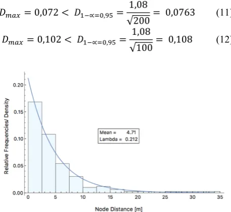
with OSM (Rostock) As a result (Figure 2 and Figure 3), both random samples are exponentially distributed with given 𝜆𝜆 (estimated by Equation 4) to be tested by the Kolmogoroff-Smirnoff-Test (KST).
Processing the KST using Equation 5 gives the results (11) for node distances and (12) for bearing differences. Both test criteria 𝐷𝐷𝑚𝑚𝑚𝑚𝜆𝜆 fall below the critical value 𝐷𝐷1−𝛼𝛼, i.e. the hypothesis that the random samples are exponentially distributed with given 𝜆𝜆 could not be declined:
𝐷𝐷𝑚𝑚𝑚𝑚𝜆𝜆 = 0,072 < 𝐷𝐷1−∝=0,95= 1,08
√200= 0,0763 (11) 𝐷𝐷𝑚𝑚𝑚𝑚𝜆𝜆 = 0,102 < 𝐷𝐷1−∝=0,95= 1,08
√100= 0,108 (12)
Figure 2. Exp. probability density function for node distances
Figure 3. Exp. probability density function for bearing differences
4.2.3 Topological evaluations
Here, the mixed random sample needs to be splitted due to the available nodes with necessary node degrees. Table 8. Random samples for topological evaluations
Node valence = 1,3 and 4 Node valence = 5 and 6 • TT (Utrecht) with OSM
(Utrecht)
• OpenData (Cologne) with OSM (Cologne) • OpenData (Rostock)
with OSM (Rostock) • OSM (Stuttgart) with
HERE (Stuttgart) • HERE (Stuttgart) with
TT (Stuttgart)
• TT (Stuttgart) with OSM (Stuttgart) • OSM (Stuttgart) with
HERE (Stuttgart) • OSM (Stuttgart) with
TT (Stuttgart)
• HERE (Stuttgart) with TT (Stuttgart)
• TT (Stuttgart) with HERE (Stuttgart) From practical point of view, for a given node valence 𝑁𝑁𝑁𝑁𝐺𝐺 in the sender system the corresponding node valence 𝑁𝑁𝑁𝑁𝐶𝐶 in a receiver system has been evaluated. This gives the results in Table 9.
Table 9. Relative frequencies of node valences
𝑁𝑁𝑁𝑁𝐶𝐶 Sample
Size
1 3 4 5 6
𝑁𝑁𝑁𝑁𝐺𝐺
1 0,97 0,03 0,00 0,00 0,00 75 3 0,00 0,84 0,16 0,00 0,00 75 4 0,00 0,17 0,83 0,00 0,00 75 5 0,00 0,07 0,64 0,29 0,00 75 6 0,00 0,10 0,54 0,22 0,14 50
Table 9 shows a nearly 1:1 matching for the common node valences 1,3 and 4. In contrast, the node valences 5 and 6 are more distributed.
As explained in detail by Hindenberger and Schwieger (2018), the general multinomial distribution for all corresponding values and a specific given value can be simplified by a binomial distribution. So, the probability 𝑒𝑒̂𝐺𝐺,𝐶𝐶 for a specific combination “given node valence – corresponding node valence” can be derived from the relative frequency 𝑓𝑓𝑟𝑟 by Equation 3.
4.2.4 Syntactical evaluations
As written in Section 3.1 this is realized as a comparison of street names which means two street names are compared to each other to find out how similar they are. To carry out such string comparation, various methods and concepts for similarity measurements can be applied. Good overviews are given in Naumann (2013) or Deza and Deza (2016). Based on this fact, a preliminary analysis has been performed to find out the best-fitting similarity measure. The analysis itself has been done on normalized strings, i.e. a given string will be transferred to a string with just upper cases, no street numbers, no space, no special (country specific) character, no abbreviations, no other symbols etc. This helps to minimize user-specific differences just by using different ways of naming a street or typical spelling/typing errors. As an outcome, the well-known and use case independent
Levenshtein distance in the variant of Damerau-Levenshtein as a normalized similarity measurement score (Equation 13 following Serva and Petroni, 2008; Naumann, 2013) has been chosen as a compromise. Basically, Levenshtein distance calculates the minimal number of operations which are necessary to transform one string into another. Every operation (insert, delete, edit) is calculated with cost = 1 which results in a sum of costs (Levenshtein, 1966; Zhang, 2009). In the variant of Damerau-Levenshtein distance, transpositions are calculated with cost = 1 (Damerau, 1964):
𝑠𝑠𝑠𝑠𝑚𝑚𝐷𝐷𝑚𝑚𝑚𝑚𝑂𝑂𝑟𝑟𝑣𝑣= 1− max(𝑠𝑠𝑒𝑒𝑟𝑟𝑠𝑠𝑓𝑓𝑠𝑠1,𝑒𝑒𝑒𝑒𝑠𝑠𝑒𝑒𝐷𝐷𝑚𝑚𝑚𝑚𝑂𝑂𝑟𝑟𝑣𝑣𝑠𝑠𝑒𝑒𝑟𝑟𝑠𝑠𝑓𝑓𝑠𝑠2) , (13)
where 𝑒𝑒𝑒𝑒𝑠𝑠𝑒𝑒𝐷𝐷𝑚𝑚𝑚𝑚𝑂𝑂𝑟𝑟𝑣𝑣= number of operations (edit distance), max(𝑠𝑠𝑒𝑒𝑟𝑟𝑠𝑠𝑓𝑓𝑠𝑠1,𝑠𝑠𝑒𝑒𝑟𝑟𝑠𝑠𝑓𝑓𝑠𝑠2)= max. length of strings.
As a result, the similarity measurements are given by a rel. frequency of 𝑓𝑓𝑟𝑟= 0,95 for 𝑠𝑠𝑠𝑠𝑚𝑚𝐷𝐷𝑚𝑚𝑚𝑚𝑂𝑂𝑟𝑟𝑣𝑣 = 100% and consequentially 𝑓𝑓𝑟𝑟= 0,05 for 𝑠𝑠𝑠𝑠𝑚𝑚𝐷𝐷𝑚𝑚𝑚𝑚𝑂𝑂𝑟𝑟𝑣𝑣 < 100% (based on the same mixed random example aggregated for the geometrical evaluations). Inserted in Equation 3, these frequencies also represent the probabilities.
4.2.5 Semantical evaluations
In Section 4.1 the semantical criteria have been introduced as supplier-dependent which means generally that for every combination of map suppliers, the distributions have to be worked out separately. Here it must be noted that this mapping is unidirectional, since the in Section 3.1 specified underlying semantical attributes are usually supplier-specific due to availability, definition, scalability, actuality and interpretation. In this paper, it has been focused on the combination TomTom with HERE, for which the distributions have been analysed. Like in Section 4.2.3 for topological evaluations, the distributions have been analysed that way that specific criteria in one system have been given and the corresponding criteria in the other system have been taken. The sample size has been selected to n=30 since by experience even a smaller sample size shows sufficient results.
As an example, the results are shown for Functional Road Class (FRC) in Table 10 and Table 11. This attribute is defined in TomTom directly as Functional Road Class (FRC) in the interval [0;8] with decreasing importance. In HERE there is a similar attribute named Functional Class (FC) and defined in the interval [1;5] with decreasing importance, too.
As Table 10 and Table 11 show, the general mapping distribution is different: In some cases (e.g. TomTom to HERE for 1 to 2), there is nearly a 1:1 matching whereas in other cases (e.g. HERE to TomTom for 3 to 1..5), the results are splitted.
Table 10. Rel. Frequencies of distribution FRC to FC HERE
1 2 3 4 5
TomTom
0 0,97 0,03 0 0 0
1 0 0,97 0,03 0 0
2 0 0,07 0,9 0,03 0
3 0 0 0,73 0,27 0
4 0 0 0,47 0,43 0,1
5 0 0,03 0,1 0,47 0,4
6 0 0 0 0,07 0,93
7 0 0 0 0,03 0,97
8 0 0 0 0 1
Table 11. Rel. Frequencies of distribution FC to FRC TomTom
0 1 2 3 4 5 6 7 8
HERE
1 0,8 0,17 0 0,03 0 0 0 0 0 2 0 0,83 0,07 0,07 0 0,03 0 0 0 3 0 0,03 0,23 0,13 0,54 0,07 0 0 0 4 0 0 0 0 0,74 0,13 0,13 0 0
5 0 0 0 0 0 0 0 0,83 0,17
5.
Experimental evaluations and results
5.1 Decision algorithm and processingTo evaluate the performance of the probability-based approach, a system has been set up that shows the absolute performance as well as the relative performance compared to a deterministic algorithm implementing the decision functions formulated in Section 3.2 using the following decision algorithm.
Table 12. Conceptual decision algorithm
Step 1 Creating a set of elements system: Edges with starting or endpoints 𝐸𝐸𝑟𝑟𝑟𝑟𝑓𝑓 in the sender representing Location Reference.
Step 2 For every element in individual set of potential candidates 𝐸𝐸𝐸𝐸𝑟𝑟𝑟𝑟𝑓𝑓: collecting an 𝑓𝑓𝑚𝑚𝑛𝑛𝑛𝑛 in the receiver system.
Step 3 For every element of this individual set of potential candidates 𝐸𝐸𝑓𝑓𝑚𝑚𝑛𝑛𝑛𝑛 : Processing the specific decision function.
Step 4
Candidate with the maximum value in this individual set 𝐸𝐸𝑓𝑓𝑚𝑚𝑛𝑛𝑛𝑛: Assumed to be the corresponding element in 𝐸𝐸𝑓𝑓𝑚𝑚𝑛𝑛𝑛𝑛 to the specific element in 𝐸𝐸𝑟𝑟𝑟𝑟𝑓𝑓.
The basic test concept consists of selecting an edge in the sender system, specifying a reference edge (reflecting to the same object) in the target system and performing the decoding process in the receiver system. The list of edges to be transferred results from real live traffic situations in Stuttgart provided by GoogleMaps.
In practice, the starting or ending edge for the given traffic situation has been identified in the sender system
and the corresponding edge (reference edge) in the receiver system has been matched manually. This has been done for the constellation of transferring TomTom to HERE as well as HERE to TomTom which results in two lists (test data) covering the same real live traffic situations. This makes it possible to compare the performance depending on the mapping direction.
As a performance indicator, the hit rate ℎ𝑟𝑟 - calculating the ratio of the number of correctly identified edges 𝑓𝑓𝑓𝑓𝑓𝑓𝑟𝑟𝑟𝑟 to all transferred edges 𝑓𝑓𝑚𝑚𝑣𝑣𝑣𝑣 – have been used (Demir, 2002):
ℎ𝑟𝑟= 𝑓𝑓𝑓𝑓𝑓𝑓𝑟𝑟𝑟𝑟
𝑓𝑓𝑚𝑚𝑣𝑣𝑣𝑣 (14)
In this context, correctly identified means that the identified edge in the receiver system is the same as the specified reference edge.
For processing the evaluations, a module in the QGIS (v 2.18.13) processing toolbox has been developed which automatically performs the decoding process.
5.2 Results
As mentioned before, two different criteria have been evaluated. First, absolute performance by probability-based main function using full set of criteria as defined in Equation 7. Processing this for a list of 𝑓𝑓𝑚𝑚𝑣𝑣𝑣𝑣= 100 edges, the hit rates in Table 13 have been obtained.
Table 13. Hit rates for probability-based main function TomTom to
HERE TomTom HERE to
Correctly identified 89 90
Not identified 11 10
Hit rate 89 % 90 %
Secondly, the relative performance by the functions for comparative calculation (Equations 8 and 9) using the reduced set of criteria. With the same list of edges as above, the hit rates are as follows (Table 14 and Table 15).
Table 14. Hit rates for comparative calculation (TomTom to HERE)
TomTom to HERE
Probability-based Deterministic
Correctly identified 87 76
Not identified 13 24
Hit rate 87 % 76 %
Table 15. Hit rates for comparative calculation (HERE to TomTom)
HERE to TomTom
Probability-based Deterministic
Correctly identified 88 75
Not identified 12 25
5.3 Analyse and assessment of the results
Generally, the overall picture of the results shows an adequate performance of the probability-based approach and gives sufficient hit rates for practical use.
For the probability-based main function, hit rates up to 90 % have been obtained with no significant difference in performance between the two mapping directions. In detail, the list of correctly identified edges slightly differs among both directions. Here, there is no specific criteria in case of no hits, but usually the combination of different criteria.
In case of the relative performance, the probability-based algorithm gives a significant higher performance, in average 12 percentage points, compared to the deterministic. Again, there is no specific criteria for the slight differences for both directions. It is noticeable here, that the hit rate between the full set of criteria (Table 13) and the reduced one (Table 14 and Table 15) is not that significant. As more in-depth analyses have shown, this is due to the predominant impact of the geometrical criteria (covered by both sets) on the overall result. From this it can be concluded that no significant improvement may be expected by adding further criteria.
6.
Conclusion
In this paper, a probability-based approach for a decision algorithm within a Location Referencing Method has been published. After giving an overview of terms and methodology in the context of Location Referencing and some mathematical principles, the specific decision functions used by the algorithm have been formulated and defined. In this, a set of criteria based on similarity measurements for geometrical, topological, syntactical and semantical attributes has been specified and the corresponding probability distributions have been estimated. The performance of these functions has been validated and confirmed by experimental evaluations based on real live traffic situations covering two mapping directions. As a conclusion, the probability-based algorithm delivers an adequate performance (up to 90% hit rate) and thus offers an improvement of 12 percentage points compared to the previous deterministic algorithms. Since this has been conducted for urban and urban hinterland scenarios, the number of uses cases could be extended by other scenarios like rural or motorway. Furthermore, elaborating another approaches to handle uncertainty are beneficial, so a fuzzy-based approach is in process.
7.
References
Bosch, K. (1986). Angewandte Statistik. Vieweg+Teubner-Verlag, Wiesbaden.
Bronstein, Semendjajew, Musiol and Mühlig (1993). Taschenbuch der Mathematik, 6. ed. Harri Deutsch Verlag, Frankfurt/Main.
Bruns, H.T. and Egenhofer, M.J. (1996). Similarity of Spatial Scenes. Seventh International Symposium on Spatial Data Handling, Delft, pp. 173–184.
Damerau, F.J. (1964). A technique for computer detection and correction of spelling errors. Commun. ACM 7, pp. 171–176.
de Lange, N. (2013). Geoinformatik, 3rd ed. Springer Berlin Heidelberg, Berlin, Heidelberg.
Demir, C. (2002). A New Location Referencing Method for Unique Reconstruction of an Object on a Second Map. Technical Paper 2175. 9th World Congress on ITS, Chicago.
Devogele, T., Trevisan, J. and Raynal, L. (1996). Building a Multi-Scale Database with Scale-Transition Relationships. Proc. of the 7th Int. Symposium on Spatial Data Handling. Advances in GIS Research II, Delft, pp. 6.19-6.33.
Deza, M. and Deza, E. (2016). Encyclopedia of distances. 4. ed. Springer, Heidelberg, New York.
Dinkelbach, W. (1969). Sensitivitätsanalysen und parametrische Programmierung, Ökonometrie und Unternehmensforschung / Econometrics and Operations Research. Springer-Verlag, Berlin, Heidelberg.
Eckey, H.-F., Kosfeld, R. and Türck, M. (2005). Wahrscheinlichkeitsrechnung und Induktive Statistik. Gabler-Verlag, Wiesbaden.
Glemser, M. (2000). Zur Berücksichtigung der geometrischen Objektunsicherheit in der Geoinformatik (Dissertation). University of Stuttgart, Stuttgart.
https://www.ifp.uni-stuttgart.de/dokumente/Dissertationen/glemser_diss.pdf. Accessed 20 may 2019.
Goodchild (1992). Geographical information science. Int. J. Geogr. Inf. Syst. 6, pp. 31–34.
Gösseln, G.V. and Sester, M. (2004). Integration of geoscientific data sets and the German digital map using a matching approach. Int. Arch. Photogramm. Remote Sens. 35, pp. 1249–1254.
GovData (2016). Straßennetz Landesbetrieb Straßenbau NRW. https://www.govdata.de/daten/-/details/ac8a18de-29d2-4bd4-ba75-6a1d4b4aabff. Accessed 1 April 2017.
Hackeloeer, A.P. (2016). Conflation of Road Networks from Digital Maps (Dissertation). TU Munich, Munich.https://mediatum.ub.tum.de/doc/1310567/13105 67.pdf. Accessed 20 May 2019.
Hagedorn, B. (2007). Design and Composition of 3D Geoinformation Services. Proceedings of the Fall 2006 Workshop of the HPI Research School on Service-Oriented Systems Engineering, Potsdam.
Hansestadt Rostock (2016). OpenData HRO.
https://www.opendata- hro.de/dataset/strassen/resource/f2a889fa-fe0e-48bf-932d-7da5c7483425. Accessed 20 May 2019.
Hartung, J., Elpelt, B. and Klösener, K.-H. (2009). Statistik: Lehr- und Handbuch der angewandten Statistik, 15. ed. Oldenbourg Verlag, München.
Interoperability Standards. Proc. Conference on Systems Engineering Research (CSER) 2007. Hoboken. Hindenberger, P. (2017). Probability Based Location
Referencing Method – Internal annual report 2017. University of Stuttgart, Stuttgart (not published). Hindenberger, P. and Schwieger, V. (2018). Probability
Based Location Referencing Method – Statistical Evaluations and Estimated Probability Distributions. Adjunct Proceedings of the 14th International Conference on Location Based Services. Zurich, pp. 7– 12.
Kenley, R. and Harfield, D.T. (2018). Scoping Study for a Location Referencing Model to Support the BIM Environment (No. AP-R568-18). Austroads Ltd., Sydney. https://austroads.com.au/publications/asset-management/ap-r568-18. Accessed 20 May 2019. Kromphardt, W., Henn, R. and Förstner, K. (1962).
Lineare Entscheidungsmodelle. Springer-Verlag, Berlin, Heidelberg.
Levenshtein, V.I. (1966). Binary Codes Capable Of Correcting Deletions, Insertions, And Reversals. Sov. Phys.-Dokl. 10, pp. 707–710.
Li, L. and Goodchild, M.F. (2012). Automatically and accurately matching objects in geospatial datasets. Adv Geo-Spat Inf Sci 10, pp. 71–79.
Lutz, M., Sprado, J., Klien, E., Schubert, C. and Christ, I. (2009). Overcoming semantic heterogeneity in spatial data infrastructures. Comput. Geosci. 35, pp. 739–752. Lv, W., Zhu, T. and Dai, X. (2008). Research of Dynamic
Location Referencing Method Based on Intersection and Link Partition. World Acad. Sci. Eng. Technol. - Int. J. Comput. Electr. Autom. Control Inf. Eng. Vol:2 (10). Ma, X., Wu, C., Carranza, E.J.M., Schetselaar, E.M., van
der Meer, F.D., Liu, G., Wang, X. and Zhang, X. (2010). Development of a controlled vocabulary for semantic interoperability of mineral exploration geodata for mining projects. Comput. Geosci. Vol: 36 (12), pp. 1512–1522.
Naumann, F. (2013). Similarity measures. Hasso Plattner Inst.
https://hpi.de/fileadmin/user_upload/fachgebiete/nauma nn/folien/SS13/DPDC/DPDC_12_Similarity.pdf. Accessed 20 May 2019.
Rodriguez, M.A. and Egenhofer, M.J. (2004). Comparing Geospatial Entity Classes: An Asymmetric and Context-Dependent Similarity Measure. Int. J. Geogr. Inf. Sci. 18, pp. 229–256.
Rommelfanger, H.J. and Eickemeier, S.H. (2002). Entscheidungstheorie, Springer-Lehrbuch. Springer Berlin Heidelberg, Berlin, Heidelberg.
Samal, A., Seth, S. and Cueto, K. (2004). A feature-based approach to conflation of geospatial sources. Int. J. Geogr. Inf. Sci. 18, pp. 459–489.
Schneebauer, C. and Wartenberg, M. (2007). On-The-Fly Location Referencing Methods for Establishing Traffic Information Services. IEEE AE Syst. Mag, pp. 14–21.
Schramm, A., Kwella, B., Schmidt, M., Pieth, N. and Ernst, T. (2012). Universal Location Referencing. Fraunhofer FIRST, Berlin.
Schützle, R. (2016). Entwicklung und Evaluierung eines formgestützten Location Referencing Verfahrens (Dissertation). University of Stuttgart, Stuttgart. http://elib.uni-stuttgart.de/handle/11682/8988. Accessed 20 May 2019.
Schwering, A. (2008). Approaches to Semantic Similarity Measurement for Geo-Spatial Data: A Survey. Trans. GIS 12, pp. 5–29.
Serva, M. and Petroni, F. (2008). Indo-European languages tree by Levenshtein distance. EPL Europhys. Lett. Vol: 81 (6).
Stadt Köln (2016). Offene Daten Köln. https://offenedaten-koeln.de/dataset/strasse. Accessed 20 May 2019.
Stigmar, H. (2005). Matching route data and topographic data in a real-time environment. 10th Scandinavian Research Conference on Geographical Information Science, Stockholm, pp. 89–107.
Streit, U. (1996). Statistical Analysis of Spatial Data in Geographic Information Systems, in: Bock, H.-H., Polasek, W. (Eds.), Data Analysis and Information Systems, Studies in Classification, Data Analysis, and Knowledge Organization. Springer Berlin Heidelberg, Berlin, Heidelberg, pp. 208–216.
Svensk, P. and Wikström, L. (2013). Georeferencing Methods - A study on how to deal with georeferencing in the ROSATTE Implementation Platform. http://tn-
its.eu/docs/emaps/eMaPS-D2.42-Triona-Georeferencing-methods-v12-130321.pdf. Accessed 20 May 2019.
TomTom B.V. (2013). OpenLR - Open, Compact and Royalty-free Dynamic Location Referencing. http://www.openlr.org/testdata.html. Accessed 20 May 2019.
Volz, S. and Walter, V. (2004). Linking different geospatial databases by explicit relations. Proceedings of the XXth ISPRS Congress, Comm. IV, Istanbul, Turkey, pp. 152–157.
Wartenberg, M. (2007). Mathematical Methods for Location Referencing (Dissertation). TU Braunschweig, Braunschweig.
Wevers, K. (2000). Improved on-the-fly Location Referencing. ITS World Congress, Turin.
Wevers, K. and Hendriks, T. (2006). AGORA-C Map-Based Location Referencing. Transp. Res. Rec. 1972, pp. 115–122.