A simple powerful bivariate test for two sample location problems in experimental and observational studies

© 2010 Tabesh et al; licensee BioMed Central Ltd. This is an Open Access article distributed under the terms of the Creative Commons Attribution License (http://creativecommons.org/licenses/by/2.0), which permits unrestricted use, distribution, and reproduction in any medium, provided the original work is properly cited.

Open Access

R E S E A R C H

Research

A simple powerful bivariate test for two sample

location problems in experimental and

observational studies

Hamed Tabesh1, S MT Ayatollahi*

and Mina Towhidi

Abstract

Background: In many areas of medical research, a bivariate analysis is desirable because it

simultaneously tests two response variables that are of equal interest and importance in two populations. Several parametric and nonparametric bivariate procedures are available for the location problem but each of them requires a series of stringent assumptions such as specific distribution, affine-invariance or elliptical symmetry.

The aim of this study is to propose a powerful test statistic that requires none of the aforementioned assumptions. We have reduced the bivariate problem to the univariate problem of sum or subtraction of measurements. A simple bivariate test for the difference in location between two populations is proposed.

Method: In this study the proposed test is compared with Hotelling's T2 _{test, two sample}

Rank test, Cramer test for multivariate two sample problem and Mathur's test using Monte Carlo simulation techniques. The power study shows that the proposed test performs better than any of its competitors for most of the populations considered and is equivalent to the Rank test in specific distributions.

Conclusions: Using simulation studies, we show that the proposed test will perform much

better under different conditions of underlying population distribution such as normality or non-normality, skewed or symmetric, medium tailed or heavy tailed. The test is therefore recommended for practical applications because it is more powerful than any of the alternatives compared in this paper for almost all the shifts in location and in any direction.

Background

Few medical research studies involve comparing two groups on only a single response vari-able; comparisons on two or more response variables are usually desired. If a single variable is identified as of major research interest, it will be appropriate to apply a two independent samples t-test or Mann-Whitney test. In some studies, however, two response variables are of equal interest and importance. For example, in studies comparing two different treat-ments for hypertension, it is equally important to compare their effects on both systolic and diastolic blood pressure. For such studies, a bivariate analysis that compares the treatments on two response variables simultaneously may have advantages over two separate univariate * Correspondence:

tests, one for each variable. The great advantage of bivariate analysis is the possibility of increased power. If the response variables are not too highly correlated, the bivariate test has a chance of finding significant differences among the treatments even if none of the univariate tests is significant [1].

In most medical research, location analysis may be sufficient and testing the distribu-tions is not necessary. For example, when it is decided to compare two characteristics of a population, such as the weight and height of infants, with those of another population, the researcher tries to compare the bivariate location in two populations. In terms of sta-tistical theory, this problem may be restated as follows.

We consider two independent random bivariate samples

(x_1i, y_1i), i = 1, ..., m and (x_2j, y_2j), j = 1, ..., n from continuous bivariate populations e.g., weight and height of infants in control and treatment populations. [X₁, Y₁]' _{and [X}

2, Y2]'

denote the joint distributions of (X₁, Y₁) and (X₂, Y₂) respectively. We intend to test

against

where δ = (δ1, δ2) ≠ (0, 0) and H0 means that the joint distribution of (X1, Y1) and (X2, Y₂) are the same.

For the above-mentioned problem, we know that for a bivariate normal population, Hotelling's T2 _{is the best. In addition, under nonsingular linear transformations, T}2 _is

invariant.

When the underlying population is unknown, many nonparametric tests have been proposed. In 1958, Blumen [2] described a sign test for the hypothesis that the medians of two or more variables had a particular value for the bivariate case. The slopes of the vector from the bivariate median to the n sample points were arranged in ascending order according to the respective angles made with the positive horizontal axis. Blumen's proposed statistic is proportional to the squared distance from the centre of gravity of the hypothesized centre. In 1962, Bennett [3] used certain properties of the multivariate normal integral to develop sign tests for the equality of means in two correlated multi-variate populations. Chatterjee and Sen [4] extended the Wilcoxon-Mann-Whitney rank sum test to the case of two variables following a conditional approach. Mardia [5] pro-posed an unconditional non-parametric statistic using the median vector of the com-bined sample. Peters and Randles [6] introduced a sign rank affine invariant test for the difference in location between two elliptically symmetric populations. Hettmansperger and Oja [7] developed a multivariate invariant sign-test for the multi-sample location problem. Sen and Mathur [8] used the angles made by centerized data for two samples with the positive direction of the x-axis to construct a test statistic suggested as an affine-invariant test statistic for the bivariate two sample location problem. Sen and

H0:

[

]

[

]

Mathur [9] proposed a consistent test similar to the Mann-Whitney test for difference in locations between two bivariate populations. LaRocque et al. [10] extended the univari-ate Wilcoxon sign rank test to the bivariunivari-ate location problem. Baringhaus and Franz [11] proposed a test statistic using the difference between the sums of all the Euclidean inter-point distances. Mathur [12] suggested a nonparametric bivariate test for two sample location problem that did not require affine-invariance or elliptic-symmetry to be assumed.

The findings of most of these tests are not easy to apply and their powers depend on the direction of shifts and the covariance matrix of the alternative distribution. Some of the proposed tests are powerful only for particular forms of distributions and some of them require specific assumptions to verify the test statistics. Thus, it seems that the tests available in the literature are not wholly adequate and hence it is necessary to intro-duce a test statistic more powerful than the existing ones, which does not depend on the covariance structure of the underlying population and is also easy to apply with readily available software for those who are not experts in statistics.

In the following section, we present a simple bivariate test statistic for the two sample location problem. To investigate the power of the proposed test and to compare it with the alternatives in the literature, a simulation study was carried out. A summary of the power study is displayed in the results and discussion sections. In the conclusion section, an application of the proposed test statistic to a real set of data is given.

Methods

Test Statistic

Let (X_1i, Y_1i) i = 1, ..., m and (X_2j, Y_2j) j = 1, ..., n be two independent random samples from bivariate populations. [X₁ Y₁]' _{and [X}

2 Y2]' denote the joint distributions of X1, Y1 and X2, Y₂ respectively. We intend to test the null hypothesis given in (1) against the alternative (2). According to the structure of this testing problem, it is presumed that the two distri-butions [X₁ Y₁]' _{and [X}

2 Y2]' have the same structural form, but there may be a location

shift in [X₂ Y₂]' _{with respect to [X}

1 Y1]'. We therefore aim to test the existence of a location

shift.

It is obvious that many tests are available to test the difference in locations between two univaraite populations. It is therefore desirable to find a convenient transformation for changing the bivariate data to the univariate case. We implement our test for three possible combinations of shift direction as follows:

(i) When the shift directions for two variables are the same i.e. δ₁ δ₂ > 0, random vari-ables are defined as S_1i = X_1i + Y_1i for i = 1, ..., m and S_2j = X_2j + Y_2j for j = 1, ..., n. Now to test the null hypothesis H0 in (1) against HA in (2), it is sufficient to test

against

′

[

]

[

]

H0: X1 Y1 ~ X2 Y2

′

[

]

[

]

where δ = δ₁ + δ₂ is a location difference parameter. In fact, this is a location problem in the univariate case and an available test such as the Mann-Whitney test can be used to solve it.

(ii) When the shift directions for two variables are not the same i.e., δ₁ δ₂ < 0, the

ran-dom variables are defined as for i = 1, ..., m and for j = 1, ..., n. Therefore, it is sufficient to test

against

Where δ = δ1 - δ2 is a location parameter. For this location problem in the univariate

case, the Mann-Whitney test is again used.

(ii) When (δ₁ = 0, δ₂ ≠ 0) or (δ₁ ≠ 0, δ₂ = 0), it is enough to apply a rank test to the sec-ond variable or the first variable, respectively.

Remark 1: To decide which of the above three methods must be used in practice, first

the values and are computed, where ,

and , . Then if > 0, method (i) is used

and if < 0, it is appropriate to use method (ii); and method (iii) is used for the test-ing problem when ( ) or ( ).

Remark 2: (a) Note that, when the two variables are on significantly different scales,

the data have to be transferred by the following relations before solving the testing prob-lem:

and

where , and and are the standard deviations of the random variables X₁ (or X₂) and Y₁ (or Y₂), respectively.

S1*i=X1i−Y1i S*2j =X2j−Y2j

′′

[

]

[

]

H₀: X₁ Y₁ ~ X₂ Y₂

′′

[

]

[

]

HA: X1 Y1 ~ X2 Y2 d

ˆ

d₁= X₁−X₂ dˆ₂=Y₁−Y₂ X _m X _i i m 1 1 1 1 = =

∑

X _n X j

j n 2 2 1 1 = =

∑

i m 1 1 1 1 = =

∑

j n 2 2 1 1 = =

∑

1 2

ˆ ˆ

d d_{1 2}

ˆ _{, ˆ}

d₁=0d₂≠0 dˆ₁≠0, ˆd₂=0

′ ′

(

)

X Y X i X

X

Y i Y Y i m i i 1 1 1 ₁ 1 1 ₁ 1 1

, m , ; ,...,

s m s ′ ′

(

)

X Y X j X

X

Y j Y

Y j n

j j 2 2 2 ₁ 1 2 ₁ 1 1

, m , ; ,...,

s

m

s

m_X E X

(b) In application, when the two variables are on significantly different scales, the data are transformed by the following relations before using a test statistic and testing hypotheses:

and

where , and , are the samples pooled variances of the first variables and the second variables in (X₁, Y₁) and (X₂, Y₂), respectively.

Power

This section indicates the results of a Monte Carlo study to assess the power of the new test. For comparison purposes, the performances of the following tests were simulated:

(1) Hotelling's T2 _{test with test statistic:}

where S-1 _{is the inverse of the sample variance-covariance matrix S [13].}

(2) The Rank test, which is based on marginal ranks, is given by

where N = m + n, i = 1, ..., N, j = 1,2, are the set of scores for each j = 1,2 and X_ij are independent identically-distributed random variables with a continuous bivariate distribution [14].

(3) The Cramer test with test statistic:

where the function ϕ is the kernel function. is recommended for location alternatives [11].

′ ′

(

)

X Y X i X

X

Y i Y Y i i

1, 1 1 1, 1 1

s s

′ ′

(

)

⎝

⎜⎜ ⎞_⎠⎟⎟

X Y X j X

X

Y j Y Y j j

2 2

2 1 2 1

, ,

s s

X _m X i

i m 1 1 1 1 = =

∑

i m 1 1 1 1 = =

∑

T2=n

{

}

{

}

R a_N R_ij j i N j = = =

∑

Rij I Xkj Xij k N = ≤ =

∑

aNj( ),...,1 aNj( )N

C mn

m n mn Xi Yj _m Xi Xj _n Yi Yj

= + ⎛⎝⎜ − ⎞⎠⎟− ⎛⎝⎜ − ⎞⎠⎟− ⎛⎝ − 2 1 2 1 2

2 2 2

f f f_⎜⎜ ⎞

⎠⎟ ⎛ ⎝ ⎜ ⎜ ⎞ ⎠ ⎟ ⎟ = =

∑

∑

∑

f_cramer

( )

ˆ ˆ

(4) The Mathur's test based on the test statistic:

where , and for i = 1, ..., m j = 1, ..., n [12].

The new proposed test (P) was compared with the above four tests using samples from bivariate normal and non-normal distributions. Simulations were run for bivariate nor-mal with ρ = -0.5,0,0.5. Also, simulations were run for some non-nornor-mal distributions generated using the g-and-h distribution [15], i.e. generating Z_ij from a bivariate normal

distribution and setting .

For g = 0 this expression is taken to be .

As the g-and-h distribution provides a convenient method for considering a very wide range of situations corresponding to both symmetric and highly asymmetric distribu-tions, its use is highly recommended. The case g = h = 0 corresponds to a normal distri-bution, the case g = 0 corresponds to a symmetric distribution, and, as g increases, the skewness increases as well. For example, with g = 0.5 and h = 0, the skewness is 1.75, which is great [16].

In this study, simulations were run with g = 0.25 and g = 0.5 to span the range of skew-ness values that seems to occur in practice.

The parameter h determines the heaviness of the tail. As h increase, the heaviness increases as well. With h = 0.2 and g = 0, the kurtosis equals 36. This might seem extreme, but even higher values were found by Wilcox, so our simulations were run for h

= 0.2 [16].

Results and discussion

The results in Table 1, Table 2, Table 3, Table 4, Table 5 and Table 6 were based on 10,000 samples of sizes 15, 18 from a bivariate population with location parameters (δ₁, δ₂). A nominal significance level of 0.05 was used. STAT, MASS, CRAMER and ICSNP librar-ies in R program version 2.10.0 were used.

Under the bivariate normal distribution with different correlations, the simulation results showed that the proposed test statistic performed better than any of the test sta-tistics compared here for almost all shifts in location.

The findings of this study show that the proposed test had greater power than Hotell-ing's T2 _{and Mathur's test for skewed populations. Also, had greater power than Cramer's}

test for a small shift in location but reached a power level equivalent to that of the Rank test for a skewed population.

M w_ij

j n

i m

=

= =

∑

∑

w_ij =I D

(

)

X_ij= gZij_g ⎛hZij

⎝ ⎜ ⎜

⎞

⎠ ⎟ ⎟

( )

exp

exp

1 2

2

X_ij =Z_ij ⎛hZij

⎝ ⎜ ⎜

⎞

⎠ ⎟ ⎟

exp

2

Table 1: Monte Carlo rejection proportion for the bivariate normal population (ρ = 0), m = 15, n = 18

δ1, δ2 P T2 R C M

0.00,0.00 0.0500 0.0511 0.0539 0.0538 0.0485

0.15,0.15 0.0878 0.0757 0.0782 0.0791 0.0529

0.15,0.25 0.1197 0.1001 0.1021 0.1034 0.0581

0.25,0.25 0.1589 0.1271 0.1289 0.1320 0.0636

0.30,0.40 0.2653 0.2160 0.2095 0.2202 0.0840

0.40,050 0.3950 0.3275 0.3189 0.3333 0.1143

0.60,0.70 0.6915 0.6069 0.5911 0.6072 0.2293

0.80,0.90 0.8951 0.8414 0.8216 0.8443 0.4327

1.10,1.30 0.9958 0.9913 0.9874 0.9912 0.8408

1.60,1.80 1.0000 0.9999 0.9999 0.9999 0.9982

0.00,0.00 0.0477 0.0511 0.0539 0.0538 0.0485

-0.15,0.15 0.0831 0.0748 0.0782 0.0756 0.0521

0.15,-0.25 0.1131 0.1060 0.1025 0.1062 0.0594

-0.25,0.25 0.1506 0.1240 0.1214 0.1235 0.0646

0.30,-0.40 0.2581 0.2118 0.2071 0.2159 0.0835

-0.40,050 0.4028 0.3254 0.3166 0.3259 0.1150

0.60,-0.70 0.6959 0.6105 0.5873 0.6106 0.2322

-0.80,0.90 0.8995 0.8477 0.8271 0.8507 0.4331

1.10,-1.30 0.9954 0.9905 0.9880 0.9907 0.8446

-1.60,1.80 1.0000 1.0000 1.0000 1.0000 0.9980

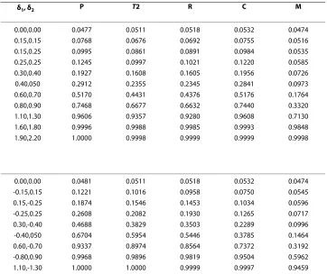
Table 2: Monte Carlo rejection proportion for the bivariate normal population (ρ = 0.5), m = 15, n = 18

δ₁, δ₂ P T2 R C M

0.00,0.00 0.0477 0.0511 0.0518 0.0532 0.0474

0.15,0.15 0.0768 0.0676 0.0692 0.0755 0.0516

0.15,0.25 0.0995 0.0861 0.0891 0.0984 0.0535

0.25,0.25 0.1245 0.0997 0.1021 0.1220 0.0585

0.30,0.40 0.1927 0.1608 0.1605 0.1956 0.0726

0.40,050 0.2912 0.2355 0.2345 0.2841 0.0973

0.60,0.70 0.5170 0.4431 0.4376 0.5176 0.1764

0.80,0.90 0.7468 0.6677 0.6632 0.7440 0.3320

1.10,1.30 0.9606 0.9357 0.9280 0.9608 0.7130

1.60,1.80 0.9996 0.9988 0.9985 0.9993 0.9848

1.90,2.20 1.0000 0.9998 0.9999 0.9999 0.9998

0.00,0.00 0.0481 0.0511 0.0518 0.0532 0.0474

-0.15,0.15 0.1221 0.1016 0.0958 0.0750 0.0545

0.15,-0.25 0.1874 0.1546 0.1453 0.1034 0.0596

-0.25,0.25 0.2608 0.2082 0.1930 0.1265 0.0717

0.30,-0.40 0.4688 0.3829 0.3503 0.2289 0.0996

-0.40,050 0.6704 0.5954 0.5446 0.3785 0.1464

0.60,-0.70 0.9337 0.8974 0.8564 0.7372 0.3192

-0.80,0.90 0.9968 0.9896 0.9819 0.9504 0.5962

When the population was highly skewed, the proposed test statistic dominated Hotell-ing's T2 _{and Mathur's test for almost all shifts in location. It also dominated Cramer's test}

for small and moderate shifts in location.

The power of the proposed test was greater than any of its competitors for almost all shifts in location except the Rank test for a large shift in location under a heavy tailed bivariate distribution.

The simulation results revealed that the proposed test statistics would perform much better when the underlying population was bivariate normal, skewed, highly skewed or heavy tailed.

The simulations were done for sample sizes m = 10 and n = 10, and the results were closely similar. In general, simulations performed for different sample sizes showed simi-lar power trends.

Conclusions

In the medical field, where two measurements such as changes in closing volume and white blood cell count [18], cholesterol level and blood pressure, potassium and sodium [19] are considered for important diagnoses, the bivariate values may be related in an unknown way, so bivariate analysis is considered an important problem. The population bivariate distributions may be unknown in many cases so parametric tests cannot be applied. Some nonparametric tests require assumptions that are hard to validate. The proposed test does not require the stringent assumption of affine-invariance or elliptic-symmetry, and it is very easy to understand and apply using only regular statistical pro-grams. In fact, we have solved the bivariate problem by reducing it to the univariate problem of sum or difference of measurements.

The results of the simulation studies showed that the proposed test performed better than most of it competitors for almost all the shifts in location. This very important property of the proposed test statistic established that it would perform much better whether the underlying population was normal or non-normal, skewed or symmetric, medium tailed or heavy tailed. Therefore, its application is recommended, since it is more powerful than any of the alternatives compared here for almost all shifts in location and in any direction.

Most of the test statistics available in the literature were difficult to compute even with the help of the computer. The proposed test statistic could easily be calculated manually for small and moderate sized data sets, which is another important property.

Table 3: Monte Carlo rejection proportion for the bivariate normal population (ρ = -0.5), m = 15, n = 18

δ1, δ2 P T2 R C M

0.00,0.00 0.0481 0.0511 0.0539 0.0526 0.0474

0.15,0.15 0.1227 0.1033 0.1016 0.0759 0.0542

0.15,0.25 0.1874 0.1528 0.1442 0.0988 0.0602

0.25,0.25 0.2671 0.2145 0.1945 0.1257 0.0685

0.30,0.40 0.4688 0.3896 0.3520 0.2284 0.0992

0.40,050 0.6774 0.5876 0.5438 0.3834 0.1448

0.60,0.70 0.9337 0.8952 0.8565 0.7368 0.3176

0.80,0.90 0.9947 0.9916 0.9826 0.9481 0.5977

1.10,1.30 1.0000 0.9999 0.9999 0.9998 0.9449

0.00,0.00 0.0477 0.0511 0.0539 0.0526 0.0474

-0.15,0.15 0.0768 0.0648 0.0688 0.0727 0.0516

0.15,-0.25 0.0928 0.0911 0.0902 0.0974 0.0553

-0.25,0.25 0.1245 0.0976 0.0990 0.1118 0.0585

0.30,-0.40 0.1902 0.1574 0.1591 0.1901 0.0743

-0.40,050 0.2912 0.2335 0.2300 0.2791 0.0959

0.60,-0.70 0.5281 0.4348 0.4325 0.5178 0.1823

-0.80,0.90 0.7468 0.6747 0.6705 0.7459 0.3300

1.10,-1.30 0.9567 0.9371 0.9295 0.9612 0.7141

-1.60,1.80 0.9996 0.9994 0.9988 0.9999 0.9847

1.90,-2.20 1.0000 1.0000 1.0000 1.0000 0.9998

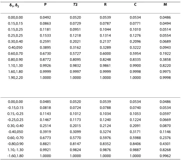
Table 4: Monte Carlo rejection proportion for the bivariate skewed population, m = 15, n = 18

δ₁, δ₂ P T2 R C M

0.00,0.00 0.0492 0.0520 0.0539 0.0534 0.0486

0.15,0.15 0.0863 0.0729 0.0787 0.0771 0.0494

0.15,0.25 0.1181 0.0951 0.1044 0.1010 0.0514

0.25,0.25 0.1533 0.1218 0.1314 0.1276 0.0554

0.30,0.40 0.2591 0.2021 0.2137 0.2096 0.0689

0.40,050 0.3895 0.3162 0.3289 0.3222 0.0943

0.60,0.70 0.6730 0.5727 0.6000 0.5954 0.1922

0.80,0.90 0.8772 0.8095 0.8248 0.8335 0.3858

1.10,1.30 0.9926 0.9832 0.9861 0.9900 0.8220

1.60,1.80 0.9999 0.9997 0.9999 0.9998 0.9975

1.90,2.20 1.0000 1.0000 1.0000 1.0000 0.9998

0.00,0.00 0.0485 0.0520 0.0539 0.0534 0.0486

-0.15,0.15 0.0818 0.0724 0.0788 0.0740 0.0534

0.15,-0.25 0.1143 0.1012 0.1034 0.1053 0.0597

-0.25,0.25 0.1467 0.1173 0.1240 0.1224 0.0669

0.30,-0.40 0.2514 0.2015 0.2124 0.2091 0.0870

-0.40,050 0.3919 0.3099 0.3274 0.3171 0.1146

0.60,-0.70 0.6773 0.5770 0.5976 0.5988 0.2376

-0.80,0.90 0.8821 0.8147 0.8352 0.8406 0.4301

1.10,-1.30 0.9921 0.9824 0.9876 0.9887 0.8268

Simultaneously, comparison of weight and height velocities between two groups of infants, with primary and secondary educated mothers, was the main interest. The bivariate observations were the 87 measurements on weight velocity (X₁) and height velocity (Y₁) over the first year of life for infants with primary educated mothers and 54 measurements on weight velocity (X₂) and height velocity (Y₂) over the first year of life for infants with secondary educated mothers.

Table 7 shows kg/mo, kg/mo, cm/mo and cm/mo. Computing and , we found that and , hence > 0. According to the sign of , method (i) should be used. So S_i = X_i + Y_i were computed for infants with primary and secondary educated mothers (i = 1,2). The Mann-Whitney test was used to test H₀: [X₁ + Y₁] ~ [X₂ + Y₂] against H_A: [X₁ + Y₁] ~ [X₂ + Y₂ + δ]; the p-value = 0.006 led to rejection of the null hypothesis at the 5% level of significance. This was consistent with the conclusion reached using Hotell-ing's T2 _{test for the same data set with p-value = 0.027.}

In order to illustrate the performance of the proposed test versus Hotelling's T2 _test

especially for small size samples, a random sample of 22 infants was selected. Weight and

X₁=0 483. X₂=0 497. Y₁=1 950.

Y₂=2 128. dˆ₁=X₁−X₂ dˆ₂=Y₁−Y₂ dˆ₁<0

ˆ

d₂<0 d dˆ ˆ_{1 2} d dˆ ˆ_{1 2}

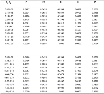
Table 5: Monte Carlo rejection proportion for the bivariate highly skewed population, m = 15, n = 18

δ1, δ2 P T2 R C M

0.00,0.00 0.0487 0.0470 0.0539 0.0532 0.0500

0.15,0.15 0.0834 0.0656 0.0834 0.0725 0.0455

0.15,0.25 0.1128 0.0836 0.1086 0.0929 0.0472

0.25,0.25 0.1478 0.1058 0.1398 0.1175 0.0501

0.30,0.40 0.2464 0.1734 0.2314 0.1942 0.0589

0.40,050 0.3664 0.2661 0.3520 0.2948 0.0777

0.60,0.70 0.6264 0.4938 0.6243 0.5627 0.1694

0.80,0.90 0.8351 0.7194 0.8386 0.8062 0.3500

1.10,1.30 0.9779 0.9429 0.9834 0.9853 0.7959

1.60,1.80 0.9991 0.9973 0.9998 0.9997 0.9933

1.90,2.20 1.0000 0.9997 1.0000 1.0000 0.9994

0.00,0.00 0.0480 0.0470 0.0539 0.0532 0.0500

-0.15,0.15 0.0796 0.0647 0.0813 0.0738 0.0531

0.15,-0.25 0.1095 0.0885 0.1088 0.0987 0.0643

-0.25,0.25 0.1412 0.1024 0.1335 0.1119 0.0657

0.30,-0.40 0.2363 0.1738 0.2270 0.1938 0.0945

-0.40,050 0.3671 0.2640 0.3479 0.2924 0.1152

0.60,-0.70 0.6272 0.4906 0.6294 0.5638 0.2400

-0.80,0.90 0.8419 0.7280 0.8437 0.8110 0.4222

1.10,-1.30 0.9812 0.9425 0.9841 0.9830 0.7890

-1.60,1.80 0.9997 0.9974 0.9998 1.0000 0.9882

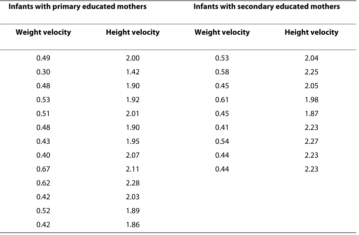
height velocities for this random sample, a part of data from Ayatollahi (2005) [17], are presented in Table 8. The bivariate observations were the 13 measurements on weight velocity (X1) and height velocity (Y1) over the first year of life for infants with primary

educated mothers and 9 measurements on X₂, Y₂ for infants with secondary educated mothers. In Table 9, mean and standard deviation of weight and height velocity over the first year of life for infants with primary and secondary educated mothers are presented.

Table 6: Monte Carlo rejection proportion for the bivariate heavy tailed population, m = 15, n = 18

δ1, δ2 P T2 R C M

0.00,0.00 0.0505 0.0470 0.0539 0.0523 0.0476

0.15,0.15 0.0754 0.0598 0.0723 0.0717 0.0535

0.15,0.25 0.0945 0.0720 0.0898 0.0890 0.0563

0.25,0.25 0.1190 0.0854 0.1091 0.1062 0.0607

0.30,0.40 0.1928 0.1379 0.1725 0.1684 0.0742

0.40,050 0.2789 0.1993 0.2570 0.2465 0.0969

0.60,0.70 0.4974 0.3782 0.4731 0.4554 0.1707

0.80,0.90 0.7167 0.5752 0.6953 0.6823 0.3050

1.10,1.30 0.9369 0.8581 0.9366 0.9326 0.6325

1.60,1.80 0.9977 0.9835 0.9985 0.9983 0.9407

1.90,2.20 0.9998 0.9976 0.9999 0.9999 0.9904

0.00,0.00 0.0480 0.0470 0.0539 0.0523 0.0476

-0.15,0.15 0.0718 0.0579 0.0722 0.0671 0.0500

0.15,-0.25 0.0921 0.0774 0.0905 0.0925 0.0573

-0.25,0.25 0.1154 0.0852 0.1059 0.0999 0.0596

0.30,-0.40 0.1849 0.1359 0.1732 0.1642 0.0750

-0.40,050 0.2743 0.2004 0.2538 0.2373 0.0980

0.60,-0.70 0.4986 0.3694 0.4717 0.4521 0.1720

-0.80,0.90 0.7236 0.5840 0.7053 0.6866 0.3011

1.10,-1.30 0.9394 0.8595 0.9373 0.9346 0.6351

-1.60,1.80 0.9965 0.9847 0.9980 0.9987 0.9436

1.90,-2.20 0.9999 0.9972 0.9999 1.0000 0.9905

Table 7: Mean and standard deviation of weight and height velocity of infants over the first year of life with primary and secondary educated mothers (m = 87, n = 54)

Mother education Weight velocity Height velocity

Primary (m = 87)

Mean 0.483 2.002

Std. Deviation 0.087 0.209

Secondary (n = 54)

Mean 0.497 2.094

Using the proposed test, the p-value was 0.030, which led to rejection of the null hypoth-esis at the 5% level of significance. However, this was not consistent with the conclusion reached using Hotelling's T2 _{test (p-value = 0.072). In this small data set, Hotelling's T}2

could not detect the difference, but the proposed test could detect it as well as in the large data set.

Table 8: Data from the weight and height velocity of infants over first year of life with primary and secondary educated mothers

Infants with primary educated mothers Infants with secondary educated mothers

Weight velocity Height velocity Weight velocity Height velocity

0.49 2.00 0.53 2.04

0.30 1.42 0.58 2.25

0.48 1.90 0.45 2.05

0.53 1.92 0.61 1.98

0.51 2.01 0.45 1.87

0.48 1.90 0.41 2.23

0.43 1.95 0.54 2.27

0.40 2.07 0.44 2.23

0.67 2.11 0.44 2.23

0.62 2.28

0.42 2.03

0.52 1.89

0.42 1.86

Table 9: Mean and standard deviation of weight and height velocity of infants over first year of life with primary and secondary educated mothers (m = 13, n = 9)

Mother education Weight velocity Height velocity

Primary (m = 13)

Mean 0.483 1.950

Std. Deviation 0.095 0.196

Secondary (n = 9)

Mean 0.493 2.128

Competing interests

The authors declare that they have no competing interests.

Authors' contributions

HT proposed the test, most of the redaction, simulation study, application to weight and height velocity. SMTA conceptu-alized and supervised the study. MT proposed the test and redaction. All authors read and approved the final manuscript.

Authors' information

Corresponding author: SMT Ayatollahi, Ph.D., FSS, C.Stat. Professor of Biostatistics, The Medical School, Shiraz University of Medical Sciences, Shiraz, Islamic Republic of Iran. P.O.Box 71345-1874

Acknowledgements

This work was supported by grant number 88-4820 from Shiraz University of Medical Sciences.

Author Details

1_{Department of Biostatistics, Shiraz University of Medical Sciences, Shiraz, Iran and} 2_{Department of Statistics, Shiraz} University, Shiraz, Iran

References

1. Fleiss JL: The Design and Analysis of Clinical Experiments. New york: John Wiley & sons; 1986. 2. Blumen I: A new bivariate sign test. Journal of American statistical Association 1958, 53:448-456. 3. Bennett B: On multivariate sign tests. Journal of the 1962, 24:159-161.

4. Chatterjee SK, Sen K: Nonparametric tests for the bivariate two sample location problem. Bull Calcutta Statist Ass 1964:18-58.

5. Mardia K: A nonparametric test for the bivariate location problem. Journal of the Royal statistical Society, series B 1967, 29:320-342.

6. Peters D, Randles R: A bivariate signed rank test for two sample location problem. Journal of American statistical Association 1991, 85:552-557.

7. Hettmansperger T, Oja H: Affine invariant multivariate multisample sign tests. Journal of Royal Statistical Society 1994, Series B(56):235-249.

8. Sen K, Mathur S: A bivariate signed rank test for two sample location problem. Commun Statist - Theory Meth 1997, 26(12):3031-3050.

9. Sen K, Mathur S: A test for bivariate two sample location problem. Commun Statist - theory Meth 2000, 29(2):417-436.

10. Larocque D, Tardif S, Eeden Cv: An affine-invariant generalization of the wilcoxon signed-rank test for the bivariate location problem. Aust N Z J Stat 2003, 45(2):153-165.

11. Baringhaus L, Franz C: On a new multivariate two-sample test. Journal of Multivariate Analysis 2004, 88:190-206. 12. Mathur SK: A new nonparametric bivariate test for two sample location problem. Stat Meth & Appl 2008,

18(3):375-388.

13. Rencher A: Methods of Multivariate Analysis. New York: John Wiley & sons; 2002. 14. Hajek J, Sidak Z, Sen KP: Theory of Rank Tests. second edition. ACADEMIC PRESS; 1999.

15. Hoaglin DC: Summarizing shape numerically: the g-and-h distributions. In Exploring Data Tables, Trends and Shapes Edited by: Hoaglin D, Mosteller F, Tukey J. New York: Wiley; 1985.

16. Wilcox RR: Simlation results on solutions to the multivariate Behrens-Fisher problem via trimmed means. The Statistician 1995, 44(2):213-225.

17. Ayatollahi SMT: Growth velocity standards from longitudinally measured infants of age 0-2 years born in Shiraz, Southern Iran. American Journal of Human Biology 2005, 17(3):302-309.

18. Merchant JA, Halprin GM, Hudson AR, Kilburn KH, McKenzie WN, Hurst DJ, Bermazohn P: Responses to Cotton Dust. Archives of Environmental Health 1975, 30:222-229.

19. Rawlings JO: Applied Regression Analysis:A Research Tool. Wadsworth, Inc.; 1988.

doi: 10.1186/1742-4682-7-13

Cite this article as: Tabesh et al., A simple powerful bivariate test for two sample location problems in experimental and observational studies Theoretical Biology and Medical Modelling 2010, 7:13

Received: 1 March 2010 Accepted: 7 May 2010 Published: 7 May 2010

This article is available from: http://www.tbiomed.com/content/7/1/13 © 2010 Tabesh et al; licensee BioMed Central Ltd.

This is an Open Access article distributed under the terms of the Creative Commons Attribution License (http://creativecommons.org/licenses/by/2.0), which permits unrestricted use, distribution, and reproduction in any medium, provided the original work is properly cited.