RESEARCH
Open Access
Scoring function to predict solubility mutagenesis
Ye Tian
1, Christopher Deutsch
2, Bala Krishnamoorthy
1*Abstract
Background:Mutagenesis is commonly used to engineer proteins with desirable properties not present in the wild type (WT) protein, such as increased or decreased stability, reactivity, or solubility. Experimentalists often have to choose a small subset of mutations from a large number of candidates to obtain the desired change, and computational techniques are invaluable to make the choices. While several such methods have been proposed to predict stability and reactivity mutagenesis, solubility has not received much attention.
Results:We use concepts from computational geometry to define a three body scoring function that predicts the change in protein solubility due to mutations. The scoring function captures both sequence and structure
information. By exploring the literature, we have assembled a substantial database of 137 single- and multiple-point solubility mutations. Our database is the largest such collection with structural information known so far. We optimize the scoring function using linear programming (LP) methods to derive its weights based on training. Starting with default values of 1, we find weights in the range [0,2] so that predictions of increase or decrease in solubility are optimized. We compare the LP method to the standard machine learning techniques of support vector machines (SVM) and the Lasso. Using statistics for leave-one-out (LOO), 10-fold, and 3-fold cross validations (CV) for training and prediction, we demonstrate that the LP method performs the best overall. For the LOOCV, the LP method has an overall accuracy of 81%.
Availability:Executables of programs, tables of weights, and datasets of mutants are available from the following web page: http://www.wsu.edu/~kbala/OptSolMut.html.
Introduction
Correlations between sequence and structure influence to a large extent how proteins fold, and also how they function. Working under this premise, most computa-tional methods used for predicting various aspects of structure and function employ scoring functions, which quantify the propensities of groups of amino acids to form specific structural or functional units. Scoring functions for mutagenesis predict the effects of changing one or more amino acids (AAs) on critical properties such as stability [1-4] or activity [5], solubility [6], etc. In experimental mutagenesis, one is often faced with the challenge of having to select a small subset from a large set of candidate mutations. Computational methods are invaluable for making such choices without generating all the mutants in the lab.
Most computationally efficient scoring functions ana-lyze protein structure at the atomic level or at the AA level. Frequencies of groups of AAs in contact have widely been used to define scoring functions for fold recognition. The default choice is two body (pairwise) contacts [7-10], but three [11,12] as well as four body contacts [13-15] have also been used to define such potential energies. It is natural to expect higher order contacts to carry more information than two body con-tacts. Further, higher order contacts could not typically be modeled by summing up the component pairwise contacts [12,16]. Four body contacts defined using the concept of Delaunay tessellation(DT) [17] of protein structures have been employed for computational muta-genesis of protein stability [3,18,19] and enzyme activity [5]. The main advantage of employing DT is that it pro-vides a more robust definition of nearest neighbors than pairwise distance calculations. DT of protein structure has also been used as a generic computational tool to analyze various aspects of protein structure such as sec-ondary structure assignment [20], structural classification * Correspondence: [email protected]
1Department of Mathematics, Washington State University, Pullman, WA
99164, USA
Full list of author information is available at the end of the article
[21,22], and analysis of small-world nature of protein contacts [23].
Even though the all-atom structure of a protein is more accurate than representing each AA by a single point, the latter approach has its advantages. Apart from being simpler, the unified residue representation can be applied even when the full-atom structure is not avail-able. This representation is also more well-suited for predicting mutagenesis, where the all-atom structure of the resulting mutant is usually not known. With protein solubility in mind, we introduce thedegree of buriedness for three body contacts under the framework of DT, which estimates the extent of surface exposure or buriedness of contacts without measuring the actual sur-face areas. Notice that an efficient method for calculat-ing solvent accessible surface areas uses alpha shapes [24], which is a generalization of DT, when working on all-atom models of proteins. At the same time, such sur-face area calculations do not consider the sequence identity of the AAs involved. On the other hand, some previous studies that included AA identities of the con-tacts have used arbitrary cut-off values on the associated solvent accessible surface areas to label the contacts as exposed or not [15]. The degrees of buriedness provides an efficient middle ground for analyzing the AA compo-sition and the buriedness of contacts in the same setting.
Compared to stability or reactivity mutagenesis, col-lections of experimental data for solubility mutagen-esis appear scarce. This is especially the case for solubility data that includes structural information. By exploring the literature, we have assembled a struc-tural dataset of 137 single- and multiple-point mutants along with the associated increases or decreases in the wild-type (WT) solubilities. To our knowledge, this is the largest structural database for solubility mutagenesis assembled so far. Some pre-vious studies [6,25,26] have developed computational models to predict whether a protein will be soluble or not. In contrast, we are predictingchanges to the solu-bility of the protein, i.e., whether solusolu-bility increases or decreases due to mutation(s). Henceforth in this paper, when we use the term predicting solubility mutagenesis, we mean the prediction of whether solu-bility increases or decreases.
We define a scoring function to predict solubility mutagenesis based on the frequencies of triplets of AAs that have low degrees of buriedness, i.e., are pre-dominantly on the surface. Machine learning techni-ques such as artificial neural networks or logistic regression [27] are often used to train such scoring functions on the experimental data. For binary classifi-cation problems, support vector machines (SVM) [28] have proven to be one of the most accurate machine
learning techniques. The method of least angle regres-sion (LAR) [29] to fit predictive models using the least absolute shrinkage and selection operator, or theLasso [30] has also gained increased popularity recently. For our dataset, we have a much larger number of triplet types (3895 descriptors) as compared to the number of proteins (137). Hence we develop a new training method based on linear programming (LP), which combines some features of SVM and the Lasso. This LP method allows us to impose meaningful bounds on the weights as part of the learning process. As such, we attain better performances than the standard SVM and Lasso classifiers.
Methods
Delaunay tessellation is a construct from computational geometry that defines clusters of nearest neighbor points based on their relative proximities (see, e.g., [17]). The dual construct of DT called theVoronoi diagramdefines convex polyhedral regions of space that are closer to the parent point than to other points. With each AA repre-sented by a single point in 3 D space, the DT describes the structure of the protein as a collection of space-fill-ing, non-overlapping tetrahedra (see Figure 1 for an illustration in 2D). These tetrahedra naturally define four body AA contacts. Solubility is predominantly a surface property, and surfaces are tessellated using trian-gles. Hence we define and analyze three body Delaunay contacts.
Figure 1Delaunay tessellation of a protein in 2D. The dots
Three-body Delaunay Contacts
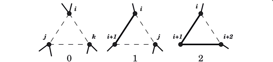
Each Delaunay tetrahedron naturally defines six edges and four triangles. We define three body AA contacts using the Delaunay triangles. We differentiate the con-tacts based on their AA composition without consider-ing the order in which the AAs occur in the protein sequence. This definition is motivated by the observa-tion that contacts are often formed by AAs distant along the backbone chain, but are close to each other in 3 D space. Backbone chain connectivity is an important aspect of the contacts, though, as demonstrated by the performance of four body scoring functions [3,14]. Hence we include backbone chain connectivity as a separate factor in the definition of three body contacts. We define three connectivity classes for three body con-tacts, having zero, one, or two bonded edges in the tri-angle (see Figure 2). We appropriately index the three body connectivity classes as 0, 1, 2. Notice that for the three body connectivity class 1, the bonded edge could either be lower down or higher up along the sequence, i.e., the residue numbers could be (i,i + 1,j) withj> i + 1, or (i,j,j+ 1), with j>i.
Delaunay Buriedness of Contacts
Surface exposure of AA contacts is typically determined by solvent accessible surface area calculations [15]. Since we use a unified residue representation, it is more nat-ural to consider levels of surface exposure from a com-binatorial point of view. Any two Delaunay tetrahedra from the DT are non-intersecting, or intersect at a tri-angle, edge, or just a vertex. Thus, each Delaunay trian-gle is shared by at most two tetrahedra. We define a triangle to beDelaunay buried, or simplyburied, if it is part of two tetrahedra in the DT. A triangle that is part of at most one tetrahedron is hence non-buried, or is on the surface. When a triangle is non-buried, we define each of its three component edges and three vertices as non-buried. To complete the definition, we say that an edge (or a vertex) is buried if it is not non-buried. Notice that the buriedness of edges is defined using the buriedness of the three body contacts of which the edge
is a component. Thus a vertex or an edge is non-buried if it is part of at least one non-buried triangle.
Once we have determined whether each vertex, edge, and triangle are buried or non-buried, we can define various levels of buriedness for two and three body con-tacts. We first introduce the case of two body buried-ness, as the buriedness of three body contacts depend on the buriedness of the component two body contacts. Further, by studying the two body case first, the reader can develop some intuition for the definitions. We define fourlevels of Delaunay buriedness for two body contacts, based on how many of the three simplices -two vertices and the edge connecting them - are buried. We appropriately index these buriedness classes by 0, 1, 2, and 3, based on the number of component simplices that are buried (see Figure 3). We also illustrate the occurrences of the two body buriedness classes in 2D in Figure 1. Interestingly, we can define the same four buriedness classes for two body contacts in three dimen-sions as well.
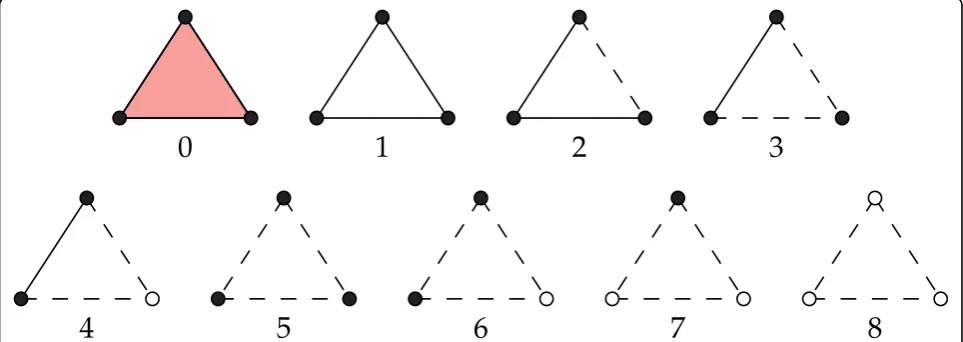
We now extend the definition of buriedness classes to three body contacts. This classification describes the various ways in which the vertices, edges, and the face of each triangle can be located on the surface of the protein, as described by its DT. For example, two ver-tices may be buried with the third one on the surface, or all three vertices and edges may be on the surface with the face buried, and so on. Altogether, there are nine buriedness classes for three body contacts (Figure 4), indexed 0-8, which range from completely non-bur-ied (class 0) to completely burnon-bur-ied (class 8).
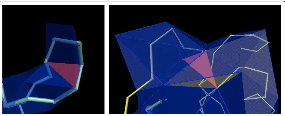
It is straightforward to visualize how some of the buriedness classes occur in proteins, for instance, classes 0, 4, or 8. But other classes may not be as intuitive, e.g., class 5 where the three vertices are on the surface, but the three edges and the triangle are buried. We illustrate buriedness classes 1 and 5 in Figure 5, which happen to be the two most rare classes. We do observe all nine classes in proteins.
Note that in defining the buriedness classes, it is not our goal to estimate any portions of the solvent
Figure 2Backbone connectivity classes for three body contacts.i,j,k, etc., are residue numbers. The connectivity indices (0, 1, 2) are
accessible surface area (SASA) [31]. One could imagine a method that estimates the fraction of SASA that is accessible to a particular residue, and defining its buriedness based on this fraction. In comparison, our simplified definition of buriedness for a single residue is given in the framework of DT. The Voronoi tessellation, which is the direct dual of DT, has been used for accu-rate SASA calculations in the past [32]. At the same time, such methods work at the atomic level rather than represent each residue by a single point. The latter method of using a unified residue representation has been utilized to speed up SASA calculations [33]. The definition of buriedness classes for groups of three resi-dues given here is combinatorial. It is different from typical SASA calculations at atomic level, and is defined specifically in the framework of DT with residues repre-sented by single points.
Distance Cutoffs
The DT is originally constructed without using any dis-tance cutoffs. Still, we need to screen the tetrahedra using a preset distance cutoff in order to define bio-chemically relevant AA contacts. We used a distance cut-off of 9 Angstroms for the 3-body contacts, in order to capture all the relevant surface features of the pro-tein. We developed the entire scoring function using a
dataset of sequentially diverse set of 3988 protein chains with at most 25% pairwise sequence identity at least 2Å resolution, selected by the PISCES server [34]. For this dataset, the relative frequencies of occurrence for the nine triplet buriedness classes 0-8 are 24.6%, 1.3%, 14.4%, 12.4%, 17.2%, 3.2%, 10.9%, 11.7%, and 4.3%, respectively. Thus, the surface triangles are the most fre-quent buriedness class. The corresponding frequencies for the three connectivity classes 0-2 were 48.2%, 43.1%, and 8.6%, respectively, showing that the non-bonded class is the most frequent one.
Assigning Buriedness ClassesThe DT is first computed using the quickhull algorithm (using code adapted from the program of [35]). The triangles are listed by running through the list of tetrahedra (four per tetrahedron). It is a non-trivial task to fix the buriedness classes of ver-tices, edges, and triangles, and we need the buriedness indices of vertices and edges to fix the same for the tri-plets. We do all the assignments as per the definitions illustrated in Figures 3 and 4 by first creating the list of all triangles, and subsequently running through the list two more times. Hence we access the entire list of trian-glesthrice.
In fact, we maintain the faces (triangles) in two sepa-rate lists - one of buried faces and the other of surface
Figure 3Buriedness classes for two body contacts. White/dotted elements are buried and black/solid elements are on the surface. Note that
in Figure 1, solid lines represent the backbone of the protein.
Figure 4Three body Buriedness classes. White/dotted elements are buried and black/solid elements are on the surface. Thus the solid
faces. We create these lists by first running through all the tetrahedra, marking the occurrences of each face in the process. If a face is spotted for the first time, we set the buriedness class of the face as non-buried (i.e., on the surface), and add it to the list of surface faces. If we spot a face for the second time, we update its buriedness class to buried, and move this face from the list of sur-face sur-faces to the list of buried sur-faces. We then make a second run through the two lists of faces in order to assign the buriedness classes of component simplices (edges and points). Note that an edge or a vertex is non-buried if is a component ofat leastone non-buried triangle. Hence we first run through the list of buried faces and mark each subsimplex as buried. We then run through the list of surface faces, and mark each subsim-plex as non-buried. The buriedness class of each vertex and edge is assigned at the end of this pass. We can now run through the lists of faces again to assign the triplet buriedness classes. We do so when we run through the list of faces for calculating the scoring func-tion. As such, we can assign the buriedness classes for all simplices and calculate scores for them in three passes through the lists of all faces. Since each tetrahe-dron in the DT contributes at most four triangles (typi-cally less, once we account for buried triangles), we can assign the buriedness classes of all simplices in O(T) time, where T is (an upper bound on) the number of tetrahedra in the DT of the protein. Notice that the space required for storing all the information pertinent to the faces is alsoO(T).
Scoring Function for Solubility Mutagenesis
DT-based scoring functions have been used for predict-ing the effects of mutations on the stability [3,18,19], and on the reactivity of proteins [5]. Computational approaches that use structural information to predict the effects of mutagenesis on protein solubility have been rare. We hypothesize that the propensities of individual or groups of amino acids to be on the surface of a protein play vital roles in determining its solubility. With the definition of buriedness classes of triplets using the DT of proteins, we have a natural way to define scoring func-tions based on groups of surface residues for predicting the effects of mutagenesis on solubility of proteins.
We generalize the four body log-likelihood score defined earlier by Krishnamoorthy and Tropsha [14] to the three body case, and add buriedness classes. The score of a triangle with amino acidsi, j,k, connectivity classc, and buriedness classbis given by
Q f
p ijk
cb ijkcb ijkcb
= ⎡
⎣ ⎢ ⎢
⎤
⎦ ⎥ ⎥
log . (1)
The frequency term
fijkcb=number of (ijk)−triplets of classes and in datac b sset total number of type triplets in datasetcb
represents the observed frequency of triangles in con-nectivity class c and buriedness class b consisting of amino acidsi,j, and kin a dataset of proteins used to
Figure 5Triplet buriedness classes 1 and 5. Instances of triplet buriedness class 1 (left) and 5 (right), shown in red. The tube represents the
develop the scoring function. The expected frequency term
pijkcb =Ca a a pi j k cb
represents the statistical expectation of encountering the triangle type, where
ai=
number of amino acids of type in dataset total number
i
o
of amino acids in dataset ,
and
pcb= cb
number of type triplets in dataset total number of trriplets in dataset .
Note that the indexc takes values 0, 1, 2, while the indexb takes values from 0-8. The combinatorial factor Caccounts for certain duplicate versions of triplets [14]. As mentioned previously under Distance Cutoffs, the log-likelihood ratios are estimated using a large, sequen-tially diverse set of proteins. This set of proteins is inde-pendent of the set of 137 solubility mutants we have assembled, which is described below.
Since we are characterizing solubility, we define the total score of a conformation as the sum of log-likeli-hood scores of individual triplets belonging to the five most non-buried classes of triangles, i.e.,b classes 0-4 (see Figure 4). We define thescoreof a mutation as the total score of the mutant conformation minus the total score of the WT. We assume the WT structure (in terms of the sidechain centers of residues) for the mutant protein as well, but the identity of the mutated residues are changed accordingly. Hence, we can calcu-late the score of a mutation by finding the change in the total score of only the subset of triangles that see a change in amino acid composition due to the mutation. Note that single and multiple point mutations are handled in a unified way by this method. Finally, we correlate a positive (negative) score of mutation with an increase (decrease) in solubility of the protein.
A dataset of solubility mutants
Scoring functions similar to ours are often optimized by learning from a training set of mutations [1,5,6]. At the same time, unlike the case of stability mutagenesis for which databases such as ProTherm [36] are already available, or reactivity mutagenesis for which some data-sets have been assembled [5], solubility mutagenesis data with structural information has not been presented in a unified manner previously. We have assembled the largest such dataset as yet, consisting of of 137 single-and multiple-point mutants along with data on changes to their solubilities. The mutants were assembled from fifteen different studies - see Table 1 for a summary.
Complete details of the dataset, including PDB codes and chain identifiers, are available in Additional File 1 (Excel), and also from the web page for the paper [37]. We identified several more studies on solubility muta-genesis (e.g., [38]), but could not include the mutants as structural information was not available for the WT.
We are predicting whether the solubility of the WT protein increases or decreases following a mutation. Hence we have tried to select mutants in the dataset that are soluble both before and after the mutation, but the extent of solubility changes. We have the info about whether the mutant is soluble for all except 16 out of 137 mutants in our dataset (this information was not available in the literature for these 16 mutants). From among the 121 mutants with info, only two were reported to become insoluble post mutation. Thus for most mutants in our dataset, the change in solubility reported is indeed an increase or a decrease in the WT solubility. We have also tried to find out what happens to the stability of the WT post mutation along with the change to its solubility. But this information appears often to be not reported in the literature for these mutants. We have this information for 26 of the mutants in the dataset, and among these mutants we see all four possible cases - with increase or decrease for both solubility and stability. As such, we believe that the changes in solubility and stability are independent for the mutants in our dataset.
Training using linear programming
For ease of notation, we index the triplets by their type t = (i, j, k,c,b), wherei, j,k are the amino acids, and c, b are the connectivity and buriedness indices. Assuming the AA composition of triplet tis changed by the mutation, its contribution to the mutation score is ± wtQt, wherewtis the weight for the log-likelihood score
Qt(Equation (1)). The sign is + if the triplet is in the
mutant and - if in the WT.
Note that the default value of each type tis wt= 1
before training, where the contribution of each triplet is weighed equally and completely. Hence we impose the bounds 0 ≤ wt ≤ 2 for each weight in our linear
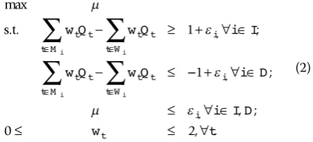
pro-gram. Similar to the optimization model used in SVMs, our objective function is to maximize the minimum margin, as shown in the LP below. In the training set of mutants, we denote the subset of instances seeing increase and decrease in solubility by I and D,
respectively. For protein i, we also denote the triplet types in the mutant that see any changes byMi, and the
same set for the WT byWi.
max
. . , ;
s t w Q w Q i I
w Q w Q
t t t t
t W t M
i
t t t t
t W t M
i i
i i
− ≥ + ∀ ∈
− ≤
∈ ∈
∈ ∈
∑
∑
∑
∑
1
−− + ∀ ∈
≤ ∀ ∈
≤ ≤ ∀
1
0 2
i
i
t
i D
i I D
w t
,
,
;
, ; , .
(2)
The variable μmodels the minimum margin over all instances, i.e., in the optimal solution, it will be equal to the smallest εivalue. Once we get the optimal weights
by solving this LP over the mutants in the training set, Table 1 Dataset of mutations studied
# Article Study Mutants Pred TOT
1 [42] Mutagenesis experiments for
APOBEC3G L260A, C261A, W168A, C281A, C288A, C308A L234A, L235A, F241A, L253A, L371A 9 11 2 [44] AA replacement improving
solubility N159D 0 1
3 [45] AA Contribution to solubility Y76 D, Y76R, Y76 S, Y76E, Y76K, Y76G, Y76A, Y76 H, Y76N, Y76P, Y76C, Y76 M, Y76V, Y76L,
Y76I, Y76F, Y76W 12 17
4 [46] mutagenesis of Ab42
s’Alzheimer’s peptide F19 D, F19E, F19N, F19R, F19Q, F19 H, F19T, F19G, F19K, F19P, F19 S, F19A, F19C, F19 M,F19W, F19Y, F19L, F19V, F19I 18 19 5 [47] Polymerization and solubility
of recombination E6F, E6W, E6L 2 3
6 [48] Genetic selection for protein
solubility (H6Q/V12A/V24A/I32M/V36G), (V12A/I32T/L34P), (V12E/V18E/M35T/I41N), (F19S/L34P), (L34P),(F4I/S8P/V24A/L34P), I32S 6 7 7 [49] Isolation of viral coat protein
mutants (A26T/I118F), N27 S, A107T (N24S/C46R/A96V/N116S), Q109L, (V48A/Q109H), I104V, (N12D/S34G/S52P/I92M/C101R/Q109L/S120T), (A21S/N24D/Q40R/V79A), (Q6L/N12D/I33T/R56C/F95L), (T15N/N24S/V29A/W32C/T45S/I60T/N98Y/I104N/S126P), (V61E/L103F/K106R/Y129H), (F4S/ W32R/Q50R)
13 13
8 [50] Improved solubility of TEV
protease (T17S/N68D/I77V), (T17S/R80S) 2 2
9 [51] Primary structure and
solubility W131A, V165K, A104T, Y203 H, W140F, C19Y, P28T, V32 M, G36R, T288 M, A384P, C70 S, C26S, C93 S, W140K, W140L, W140C, (W86F/W140F), (W130F/W140F), P28K, H44Y, (W86F/W130F/ W140F), R68C, G346 S, G349 S, A198V
21 26
10 [52] Substitutions affecting
protein solubility K97R, (K113F/W140K), (K113F/W140L), (K113F/W140C), K63 M, L104 M, T90A, L87 M, (T90A/E97A), L127 M, V74F, E97A, K69 M, (T345L/M358R), M358L, K97G, K97V, W140C, L10N, L10 D, L10T
12 21
11 [53] Dual selection for
functionally active mutants (Y35Q/F37R), (Y35L/F37T), (Y35G/F37L), (Y35L/F37R), K27E 4 5 12 [54] Assay for increased protein
solubility K185F, K185I, K185V, K185L, K185N, K185D 6 6
13 [55] Phage T4 vertex protein
gp24 (E89A/E90A) 1 1
14 [56] Human cell surface receptor
CD58 (Q21V/S85T/S1F/K9V/K58V/G93L) 1 1
15 [57] Solubility and folding of a
genetic marker W232E, Y242E, I317E, (G32D/I33P) 4 4
the score of a test protein j is calculated as
sj w Qt w Qt t
t Mj t t wj
= −
∈ ∈
∑
∑
, after setting wt = 1for any singleton triplet type t. The solubility of the test protein is predicted to increase if sj > 0 and
decrease ifsj< 0.
Comparison to SVM and Lasso models
The standard optimization model used by SVM does not impose any bounds on the weights wt. In our LP
model, the weights of triplet types that are critical to the determination of solubility are closer to 2, while the unimportant triplets get weights assigned close to zero. Since a singleton triplet does not appear in any of the training set proteins, its value will be set to zero by the LP. In comparison, SVM methods using both linear and nonlinear kernels assign nonzero values to these weights. The key modification we make is to reset the singleton weights to the default value of 1, and use the remaining weights as set by the LP when calculatingsj.
Equivalently, we can incorporate this change in the weights of singleton triplets by replacing each occur-rence ofwtin the LP (2), and subsequently in the
calcu-lation of sj , by wt + 1. The minimum margin of
separation for positive and negative data instances may not be equal in our LP, while the SVM separating hyperplane typically has the same minimum margin for both classes. If a perfect separation of all mutants in the training set into cases of increase and decrease in solu-bility exists, the optimal value ofμwill be non-negative. Further, the larger the value of μ> 0 is, the better the separation margin is. Also, the objective function for the LP is linear, while it is quadratic for SVM even when using the linear kernel.
The idea of imposing bounds on regression coeffi-cients has been used previously in the Lasso regression [30], but this procedure tries a range of values for these bound(s) by creating a family of models. It then chooses the best bound(s) using cross validation. In contrast, the bounds we impose are very specific to the case of the scoring function in question, and we also do not con-sider a sequence of bounds. We compare our LP method to the least angle regression method [29] for building Lasso models for logistic regression. Similar to the optimization model of SVMs, the objective function in the Lasso model is also non-linear.
Cross validation across sequentially diverse folds
As an alternative method of cross validation, we con-sidered the division of the dataset of 137 mutants into various subsets or folds based on sequence similarity. The idea is to explore the robustness of the scoring function across sequentially diverse families of pro-teins. The full dataset of mutants include 19 different PDB entries, and hence we first consider k= 19 folds
with one protein (i.e., one PDB file) per fold. As one would expect, the mutants of the same protein are classified in the same fold according to measures of sequence similarity. When leaving one fold out for the purpose of training and testing, there are many single-ton triplets. Hence we are not able to assign the weights of these triplets effectively, as they do not appear in the training set of mutants. Hence we gradu-ally increase the number of folds for the purpose of training and testing, with the folds still created based on sequence alignment scores. We employed the sequence alignment functions available as part of the Bioinformatics toolbox in MATLAB to create the folds. We considerk = 30, 50, andk= 70 folds in this analysis. These folds are made available in Additional File 3 as well as on the web page for the paper. Comparison to hydrophobicity valuesWe have calcu-lated the average hydrophobicity values of the mutation site residues before and after mutation according to the definitions of Varadarajan et al. [39]. The changein average hydrophobicity of residue j is calculated as
HavMut( )j −HavWT( )j , where Hav(j) is calculated as an average over a window of 7 residues (Equation [2] in the original paper [39]). We want to see if changes in solubility are correlated to changes in hydrophobicity values of the mutated residues. For multipoint muta-tions, we average the per-residue average hydrophobicity changes over all mutation sites. Ideally, hydrophobicity values would be expected to decrease when solubility increases, as the protein attracts more water.
Results
Previous computational studies related to our line of work have tried to predict whether the protein will be soluble or not after mutation, rather than predict the change in its solubility. We still mention these results briefly. Smialowski et al. [25] have summarized the accuracies of most of these methods, all of which use only sequence-based attributes. They reported an overall accuracy of 70%, while Idicula-Thomas et al. [6] reported a slightly higher accuracy of 72%, which has been the best reported accuracy so far (these authors used a different dataset of 64 mutants).
best model for logistic regression (we choose the family as binomial) by using 10-fold cross validation on the training set alone. Thus we use 10-fold CV as the proce-dure for model selection within LAR when performing LOO, 10-fold, and 3-fold CV on the overall set of mutants. The best model thus selected in each case is then used to predict the classes for the mutants in the test set.
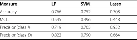
We report the accuracy, Matthew’s correlation coeffi-cient (MCC) [41], and precisions for both classes for each model. The statistics for LOOCV are presented in Table 2, those for 10-fold CV are presented in Table 3, and those for 3-fold CV are presented in Table 4. These statistics show that the LP method outperforms SVM and Lasso classifiers based on all three CV methods. We used the default linear kernel for the SVM classifier. All nonlinear kernel options available in LibSVM performed worse than the linear kernel in this case, typically pre-dicting all, or most, of the mutants to be in one class. The confusion matrices for LP, SVM, and Lasso predic-tion models are provided in Addipredic-tional File 2.
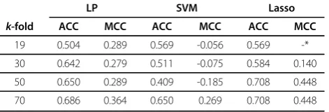
Fork-fold cross validation across sequentially diverse folds, we report the accuracy and MCC values for k= 19, 30, 50, 70 in Table 5. These folds are created using sequence alignment scores, thus grouping mutants with similar sequences in the same fold. For k= 19, which corresponds to leaving one protein out, the perfor-mances are not great. There are many singleton triplets under this setting, for which the optimal weights cannot be assigned by learning. The performances are better when we go tok= 30 folds, with the LP method achiev-ing an accuracy of 0.64 and an MCC value of 0.28. When the number of folds is increased further, the per-formances are expectedly better, as the number of sin-gleton triplets go down. For k = 50 folds, the Lasso models outperformed the LP models, achieving an accu-racy of 0.71 and an MCC value of 0.45. In summary, the scoring functions are effective as long as we can assign weights under training for a big majority of the triplet types. No obvious correlation was observed between the changes in hydrophobicity and solubility values for our dataset of mutants. 36 out of 78 mutants seeing a decrease in solubility show an increase in hydrophobi-city, and 42 out of 59 mutants with increasing solubility showed a decrease in hydrophobicity. The detailed
results are available in Additional File 3 (Excel) and in the web page for the paper [37].
Conclusions
This study demonstrates that the default settings avail-able as part of standard machine learning methods may not be appropriate for all data sets. Our LP-based method could be applied to other similar datasets, in which over-fitting may be a concern due to a large number of descriptors as compared to the number of entries in the training set. At the same time, it may not be obvious what the default weight or the bounds should be for other datasets. One could also implement the flexible treatment of weights as part of the optimiza-tion framework of an SVM model.
We are trying to expand out dataset of solubility mutants by further exploration of literature. We have already found a few mutants whose solubility is reported to be “close to WT"- for example, some mutants from the study of Chen et al. [42] (which are not included in our dataset). One way to include such mutants in our study is to expand the underlying model to include a third class of mutants that seeno changein solubility post mutation. The prediction models would then have to be developed for multiclass prediction - 3-class to be exact, into I, D, and N for no change. At this point, we do not have a sizable number of mutants in the N class, but we plan to identify enough such mutants in the near future. At the same time, it may not be obvious how the LP model can be modified easily to handle more than two classes. The default idea would be to try the one-versus-all strategy, as used in multiclass SVM [40].
For the binary classification case, we expect the LP method to be effective even on larger datasets. The total number of triplet types considered in the scoring Table 3 Statistics for 10-fold CV using LP, SVM, and Lasso models
Measure LP SVM Lasso
Accuracy 0.766 0.752 0.708
MCC 0.545 0.496 0.448
Precision(classI) 0.719 0.705 0.952
Precision(classD) 0.822 0.790 0.664
Table 4 Statistics for 3-fold CV using LP, SVM, and Lasso models
Measure LP SVM Lasso
Accuracy 0.766 0.686 0.715
MCC 0.529 0.359 0.452
Precision(classI) 0.714 0.638 0.917
Precision(classD) 0.811 0.722 0.673
Table 2 Statistics for LOOCV using LP, SVM, and Lasso models
Measure LP SVM Lasso
Accuracy 0.810 0.708 0.701
MCC 0.617 0.405 0.423
Precision(classI) 0.762 0.661 0.909
function is 1540 × 3 × 5 = 23100 (using 20 AAs, 3 connectivity classes, and 5 buriedness classes). Even with a few thousands of mutants in the dataset, one could expect the number of triplets seeing any changes to be larger than the number of mutations themselves. Hence, one could still hope for a complete separation of the three classes when solving the LP for the entire dataset. The current dataset is diverse, but one could re-train the weights by solving the LP on a specific family of proteins, if the goal is prediction for mutants belonging to the same family. This scoring function should perform better on test proteins within the family than the default scoring function, and poorer on ones outside it. Our method handles single- and multi-ple-point mutants in the same manner. In fact, it may be more accurate on multiple-point mutants, as the number of triplets involved in the mutation will typi-cally be larger.
Additional material
Additional file 1: Dataset of solubility mutants. PDB code, chain,
mutation details, and information about whether solubility increased or decreased for each of 137 mutants in the dataset. Information about whether the wild type and the mutant were soluble is included. Further, info on whether stability increased, was unchanged, or decreased due to the mutations is also included when available. Predictions by the linear programming (LP) model under leave-one-out cross validation are also listed for each mutant. Format: Excel file.
Additional file 2: Confusion Matrices. The confusion matrices for
predictions using LP, SVM, and Lasso using leave-one-out, 10-fold, and 3-fold cross validation (9 tables).
Additional file 3: Cross validation across sequentially diverse folds.
Divisions of the dataset into 19, 30, 50, and 70 folds based on sequence similarity of the mutants. Analyses of predictions using LP, SVM, and Lasso methods for each division. Accuracy and MCC of predictions reported for each case. Also included is the comparison of solubility changes to changes in average hydrophobicity values. Format: Excel file.
Acknowledgements
Krishnamoorthy and Deutsch are thankful for the support provided by the NSF Grant EF 0531870 for working on the research presented in this paper.
Author details
1Department of Mathematics, Washington State University, Pullman, WA
99164, USA.2Department of Chemistry, Portland State University, Portland,
OR 97207, USA.
Authors’contributions
YT carried out all the calculations presented in this paper. Some code for the three body scoring function was written by BK. CD carried out the exhaustive literature search to assemble the dataset of mutants. BK supervised all work, and also did the majority of work on writing the paper. YT had some contributions to the writing as well.
All three authors have read and approved the final manuscript.
Authors’Information
BK is an assistant professor in Mathematics, and YT is a PhD student in Mathematics working under BK. BK has done previous work on scoring functions for proteins. CD is currently a graduate student in Biochemistry, and did research under BK as an undergraduate student previously. Part of the work related to the assembly of mutant data set was done by CD when he was an undergraduate student.
Competing interests
The authors declare that they have no competing interests.
Received: 1 June 2010 Accepted: 7 October 2010 Published: 7 October 2010
References
1. Dehouck Y, Grosfils A, Folch B, Gilis D, Bogaerts P, Rooman M:Fast and accurate predictions of protein stability changes upon mutations using statistical potentials and neural networks: PoPMuSiC-2.0.Bioinformatics
2009,25(19):2537-2543.
2. Cheng J, Randall A, Baldi P:Prediction of protein stability changes for single-site mutations using support vector machines.Proteins: Structure, Function, and Bioinformatics2006,62(4):1125-1132.
3. Deutsch C, Krishnamoorthy B:Four-body scoring function for mutagenesis.Bioinformatics2007,23(22):3009-3015.
4. Capriotti E, Fariselli P, Rossi I, Casadio R:A three-state prediction of single point mutations on protein stability changes.BMC Bioinformatics2008, 9(Suppl 2):S6, online.
5. Masso M, Vaisman II:Accurate prediction of enzyme mutant activity based on a multibody statistical potential.Bioinformatics2007, 23(23):3155-3161.
6. Idicula-Thomas S, Kulkarni AJ, Kulkarni BD, Jayaraman VK, Balaji PV:A support vector machine-based method for predicting the propensity of a protein to be soluble or to form inclusion body on overexpression in Escherichia coli.Bioinformatics2006,22(3):278-284.
7. Miyazawa S, Jernigan RL:Residue-residue potentials with a favorable contact pair term and an unfavorable high packing density term, for simulation and threading.Journal of Molecular Biology1996, 256(3):623-644.
8. Sippl MJ:Calculation of conformational ensembles from potentials of mean force.Journal of Molecular Biology1990,213:859-883.
9. Samudrala R, Moult J:An all-atom distance-dependent conditional probability discriminatory function for protein structure prediction. Journal of Molecular Biology1998,275(5):895-916.
10. Li X, Hu C, Liang J:Simplicial edge representation of protein structures and alpha contact potential with confidence measure.Proteins: Structure, Function, and Bioinformatics2003,53(4):792-805.
11. Banavar JR, Maritan A, Micheletti C, Trovato A:Geometry and physics of proteins.Proteins: Structure, Function, and Genetics2002,47(3):315-322.
12. Li X, Liang J:Geometric cooperativity and anticooperativity of three-body interactions in native proteins.Proteins: Structure, Function, and
Bioinformatics2005,60:46-65.
13. Singh RK, Tropsha A, Vaisman II:Delaunay tessellation of proteins: Four body nearest neighbor propensities of amino acid residues.Journal of Computational Biology1996,3(2):213-222.
14. Krishnamoorthy B, Tropsha A:Development of a four-body statistical pseudo-potential for discriminating native from non-native protein conformations.Bioinformatics2003,19(12):1540-1549.
Table 5 Accuracy and MCC values fork-fold CV using LP,
SVM, and Lasso models, when the folds are created using sequence similarity scores
LP SVM Lasso
k-fold ACC MCC ACC MCC ACC MCC
19 0.504 0.289 0.569 -0.056 0.569 -*
30 0.642 0.279 0.511 -0.075 0.584 0.140
50 0.650 0.289 0.409 -0.185 0.708 0.448
70 0.686 0.364 0.650 0.269 0.708 0.448
15. Feng Y, Kloczkowski A, Jernigan RL:Four-body contact potentials derived from two protein datasets to discriminate native structures from decoys. Proteins: Structure, Function, and Bioinformatics2007,68:57-66.
16. Ben-Naim A:Statistical potentials extracted from protein structures: Are these meaningful potentials?The Journal of Chemical Physics1997, 107(9):3698-3706.
17. Edelsbrunner H:Geometry and Topology for Mesh GenerationCambridge University Press, England 2001.
18. Jr CW, LeFebvre B, Cammer SA, Tropsha A, Edgell MH:Four-body potentials reveal protein-specific correlations to stability changes caused by hydrophobic core mutations.Journal of Molecular Biology2001, 311:625-638.
19. Masso M, Lu Z, Vaisman II:Computational Mutagenesis Studies of Protein Structure-Function Correlations.Proteins: Structure, Function, and Bioinformatics2006,64:234-245.
20. Taylor TJ, Rivera M, Wilson G, Vaisman II:New method for protein secondary structure assignment based on a simple topological descriptor.Proteins: Structure, Function, and Bioinformatics2005, 60(3):513-524.
21. Bostick DL, Shen M, Vaisman II:A simple topological representation of protein structure: Implications for new, fast, and robust structural classification.Proteins: Structure, Function, and Bioinformatics2004, 56(3):486-501.
22. Huan J, Bandyopadhyay D, Wang W, Snoeyink J, Prins J, Tropsha A:
Comparing Graph Representations of Protein Structure for Mining Family-Specific Residue-Based Packing Motifs.Journal of Computational Biology2005,12(6):657-671.
23. Taylor TJ, Vaisman II:Graph theoretic properties of networks formed by the Delaunay tessellation of protein structures.Physical Review E (Statistical, Nonlinear, and Soft Matter Physics)2006,73(4):041925.
24. Edelsbrunner H, Koehl P:The geometry of biomolecular solvation. Combinatorial and Computational GeometryMSRI Publications 2005,
52:243-275.
25. Smialowski P, Martin-Galiano AJ, Mikolajika A, Girschick T, Holak TA, Frishman D:Protein solubility: sequence based prediction and experimental verification.Bioinformatics2007,23(19):2536-2542.
26. Wilkinson DL, Harrison RG:Predicting the Solubility of Recombinant Proteins in Escherichia coli.Nature Biotechnology1991,9:443-448.
27. Mitchell TM:Machine LearningMcGraw Hill, 1 1997. 28. Vapnik VN:Statistical Learning TheoryWiley and Sons Inc 1998. 29. Efron B, Hastie T, Johnstone I, Tibshirani R:Least angle regression.Annals
of Statistics2004,32:407-499.
30. Tibshirani R:Regression Shrinkage and Selection via the Lasso.Journal of the Royal Statistical Society, Series B (Methodological)1996,58:267-288.
31. Lee B, Richards F:The interpretation of protein structures: Estimation of static accessibility.Journal of Molecular Biology1971,55(3):379-400, IN3-IN4.
32. McConkey B, Sobolev V, Edelman M:Quantification of protein surfaces, volumes and atom-atom contacts using a constrained Voronoi procedure.Bioinformatics2002,18(10):1365-1373.
33. Cavallo L, Kleinjung J, Fraternali F:POPS: a fast algorithm for solvent accessible surface areas at atomic and residue level.Nucleic Acids Research2003,31(13):3364-3366.
34. Wang G, Jr R:PISCES: a protein sequence culling server.2003.
35. Watson D:CONTOURING: A guide to the analysis and display of spatial data
Pergamon Press 1992.
36. Kumar MS, Bava KA, Gromiha MM, Prabakaran P, Kitajima K, Uedaira H, Sarai A:ProTherm and ProNIT: thermodynamic databases for proteins and protein-nucleic acid interactions.Nucleic Acids Research2006,34:
D204-D206.
37. Supplementary Materials and Executable programs for this paper.
[http://www.wsu.edu/~kbala/OptSolMut.html].
38. Liu J, Boucher Y, Stokes H, Ollis D:Improving protein solubility: the use of the Escherichia coli dihydrofolate reductase gene as a fusion reporter. Protein Expression and Purification2006,47:258-63.
39. Varadarajan R, Nagarajaram H, Ramakrishnan C:A procedure for the prediction of temperature-sensitive mutants of a globular protein based solely on the amino acid sequence.Proceedings of the National Academy of Sciences of the United States of America1996,93(24):13908-13913.
40. Chang CC, Lin CJ:LIBSVM: a library for support vector machines2001 [http:// www.csie.ntu.edu.tw/~cjlin/libsvm].
41. Matthews B:Comparison of the predicted and observed secondary structure of T4 phage lysozyme.Biochem Biophys Acta 4051975, 442-451.
42. Chen KM, Martemyanova N, Lu Y, Shindo K, Matsuo H, Harris RS:Extensive mutagenesis experiments corroborate a structural model for the DNA deaminase domain of APOBEC3G.FEBS letters2007,581:4761-4766.
43. Humphrey W, Dalke A, Schulten K:VMD - Visual Molecular Dynamics. Journal of Molecular Graphics1996,14:33-38.
44. Dale GE, Broger C, Langen H, Arcy AD, Stüber D:Improving protein solubility through rationally designed amino acid replacements: solubilization of the trimethoprim-resistant type S1 dihydrofolate reductase.Protein Eng1994,7(7):933-939.
45. Trevino SR, Scholtz J, Pace C:Amino Acid Contribution to Protein Solubility: Asp, Glu, and Ser Contribute more Favorably than the other Hydrophilic Amino Acids in RNase Sa.Journal of Molecular Biology2007, 366(2):449-460.
46. de Groot N, Aviles F, Vendrell J, Ventura S:Mutagenesis of the central hydrophobic cluster in Ab42 Alzheimer’s peptide.FEBS Journal2006, 273(3):658-668.
47. Adachi K, Konitzer P, Kim J, Welch N, Surrey S:Effects of beta 6 aromatic amino acids on polymerization and solubility of recombinant hemoglobins made in yeast.The Journal of Biological Chemistry1993, 268:21650-21656.
48. Fisher A, Kim W, DeLisa M:Genetic selection for protein solubility enabled by the folding quality control feature of the twin-arginine translocation pathway.Protein Science2006,15(3):449-58.
49. Peabody DS, Al-Bitar L:Isolation of viral coat protein mutants with altered assembly and aggregation properties.Nucleic Acids Research2001, 29(22):e113.
50. van den Berg S, Löfdahl PÅ, Härd T, Berglund H:Improved solubility of TEV protease by directed evolution.Journal of Biotechnology2006, 121(3):291-298.
51. Idicula-Thomas S, Balaji PV:Understanding the relationship between the primary structure of proteins and its propensity to be soluble on overexpression in Escherichia coli.Protein Sci2005,14(3):582-592.
52. Sim J, Sim T:Amino acid substitutions affecting protein solubility: high level expression of streptomyces clavuligerus isopenicillin N synthase in Escherichia coli.Journal of Molecular Catalysis B: Enzymatic1999, 6(3):133-143.
53. Japrung D, Chusacultanachai S, Yuvaniyama J, Wilairat P, Yuthavong Y:A simple dual selection for functionally active mutants of Plasmodium falciparum dihydrofolate reductase with improved solubility.Protein Eng Des Sel2005,18(10):457-64.
54. Maxwell KL, Mittermaier AK, Forman-Kay JD, Davidson AR:A simple in vivo assay for increased protein solubility.Protein Science1999,8(9):1908-1911.
55. Boeshans K, Liu F, Peng G, Idler W, Jang S, Marekov L, Black L, Ahvazi B:
Purification, crystallization and preliminary X-ray diffraction analysis of the phage T4 vertex protein gp24 and its mutant forms.Protein Expr Purif
2006,49(2):235-43.
56. Sun ZYJ, Dotsch V, Kim M, Li J, Reinherz EL, Wagner G:Functional glycan-free adhesion domain of human cell surface receptor CD58: design, production and NMR studies.The EMBO journal1999,18(11):2941-9.
57. Wigley WC, Stidham RD, Smith NM, Hunt JF, Thomas PJ:Protein solubility and folding monitored in vivo by structural complementation of a genetic marker protein.Nature Biotechnology2001,19:131-136.
doi:10.1186/1748-7188-5-33
Cite this article as:Tianet al.:Scoring function to predict solubility