www.the-cryosphere.net/6/467/2012/ doi:10.5194/tc-6-467-2012
© Author(s) 2012. CC Attribution 3.0 License.
The Cryosphere
Repeat optical satellite images reveal widespread and long term
decrease in land-terminating glacier speeds
T. Heid and A. K¨a¨ab
Department of Geosciences, University of Oslo, Box 1047 Blindern, 0316 Oslo, Norway Correspondence to: T. Heid ([email protected])
Received: 17 October 2011 – Published in The Cryosphere Discuss.: 31 October 2011 Revised: 15 March 2012 – Accepted: 19 March 2012 – Published: 10 April 2012
Abstract. By matching of repeat optical satellite images it is now possible to investigate glacier dynamics within large regions of the world and also between regions to improve knowledge about glacier dynamics in space and time. In this study we investigate whether the negative glacier mass bal-ance seen over large parts of the world has caused the glaciers to change their speeds. The studied regions are Pamir, Cau-casus, Penny Ice Cap, Alaska Range and Patagonia. In ad-dition we derive speed changes for Karakoram, a region as-sumed to have positive mass balance and that contains many surge-type glaciers. We find that the mapped glaciers in the five regions with negative mass balance have over the last decades decreased their velocity at an average rate per decade of: 43 % in the Pamir, 8 % in the Caucasus, 25 % on Penny Ice Cap, 11 % in the Alaska Range and 20 % in Patagonia. Glaciers in Karakoram have generally increased their speeds, but surging glaciers and glaciers with flow instabilities are most prominent in this area. Therefore the calculated aver-age speed change is not representative for this area.
1 Introduction
Deriving glacier surface velocities from optical satellite im-ages using image matching is well established within glaciol-ogy. In the beginning manual methods were used (Luc-chitta and Ferguson, 1986), but later automatic techniques took over. Bindschadler and Scambos (1991) and Scambos et al. (1992) were the first to use automatic image match-ing techniques to derive glacier velocities. They used nor-malized cross-correlation (NCC) based on the work of Bern-stein (1983), where some of the terms are solved using Fast Fourier Transform (FFT). Later, different image match-ing techniques have been applied for this purpose. Most
studies have used the NCC technique (e.g. Scambos et al., 1992; K¨a¨ab, 2002; Copland et al., 2009; Skvarca et al., 2003; Berthier et al., 2005), some have used least square matching (Kaufmann and Ladst¨adter, 2003; Debella-Gilo and K¨a¨ab, 2011b), and lately methods correlating only in the frequency domain have become more common (Rolstad et al., 1997; Scherler et al., 2008; Haug et al., 2010; Herman et al., 2011; Quincey and Glasser, 2009) especially after the development of COSI-Corr (Leprince et al., 2007).
Most studies have focused on specific glaciers or smaller glacier regions, and only a few studies so far have focused on deriving glacier surface velocities for larger regions and comparing those (K¨a¨ab, 2005; Copland et al., 2009; Scher-ler et al., 2011a,b; McFadden et al., 2011). However, much focus has lately been put into developing, improving and automating image matching techniques to make them well suited for image matching of glaciers (e.g. Leprince et al., 2007; Debella-Gilo and K¨a¨ab, 2011a,c; Haug et al., 2010; Heid and K¨a¨ab, 2012; Scherler et al., 2008) and also on com-paring image matching techniques to find the methods that produce best results for glaciers (Heid and K¨a¨ab, 2012). It is therefore now possible to focus on comparing glacier veloci-ties within large regions and also between regions to improve our knowledge about glacier dynamics and its variation in space and time.
slow down, at least on regional averages. To test this hypoth-esis, we select five glacier regions where the mass balance has been negative over the last decades. These regions are Pamir, Caucasus, Penny Ice Cap, Alaska Range and Southern Patagonia Ice Field (Fig. 1). The mass balances of these re-gions are listed in Table 1. Other mass balance estimates also exist for some of these regions, but we choose the most recent estimates. In addition we also select Karakoram in Himalaya, where glaciers are assumed to have had a positive mass bal-ance over the last years (Hewitt, 2005), and measured glacier speed increases at Baltoro glacier are assumed to be asso-ciated with this mass surplus (Quincey et al., 2009a). The Karakoram area is also known for its many surging glaciers (Hewitt, 1969, 2007; Copland et al., 2009; Quincey et al., 2011; Copland et al., 2011).
The glaciers in the studied regions are mainly alpine and land-terminating, and they are influenced by different cli-matic conditions. Glaciers on the southern side of the Alaska Range experience a maritime climate, as well as glaciers of the western sides of the Southern Patagonia Ice Field. The other regions have a more continental climate. We can only select areas were it is possible to derive yearly speeds for two periods separated by more than a decade, and hence the availability of Landsat images also influences the selection. Karakoram is chosen because Baltoro glacier has increased its speed during the last years (Quincey et al., 2009a) possi-bly due to positive mass balance, and we therefore want to investigate whether this is also the case for other glaciers in this region. In addition we want to look into the temporal and spatial variability in glacier speeds in Karakoram.
The aim of this study is to test if, and to what degree, glacier speeds have decreased on regional scales due to nega-tive mass balance. Such a relationship is well expected, but it has never been observed on regional scales before. Quincey et al. (2009b) derived speeds for six glaciers in the Himalaya region between 1992 and 2002, but these data show no clear sign of a reduction in speed with time. A reduction in speed in areas with negative mass balance has been observed for in-dividual glaciers using ground observations (Haefeli, 1970; Span and Kuhn, 2003; Vincent et al., 2009), but also increase in speed in areas with negative mass balance has been ob-served (Vincent et al., 2000). Because glaciers may behave very differently even though they experience the same cli-matic conditions, the relationship between mass balance and speed should not only be studied for individual glaciers, but also for entire regions.
2 Methods
Most previous studies that have investigated glacier ve-locities on regional scales using optical images have used ASTER images. One exception is McFadden et al. (2011), who also used Landsat images. We use Landsat images for this study because of the advantages given below. Sensor
specifications are listed in Table 2. The main advantages of Landsat are that one Landsat image covers a 9-fold larger area than an ASTER image, and that they extend back to 1972. The latter makes it possible to study long-term veloc-ity changes. We should however note that it is also possible to combine ASTER and Landsat data in the kind of study per-formed here (K¨a¨ab et al., 2005b). Landsat images are also used in other studies of global glacier changes, like Global Land Ice Measurements from Space (GLIMS) (Bishop et al., 2004; Kargel et al., 2005; Raup et al., 2007), GlobGlacier and Glacier CCI. The use of Landsat data for glacier veloc-ity measurements thus ensures a consistency in source data for the various glacier parameters derived, and a larger com-bined automation potential. Landsat images are available at no cost through the US Geological Survey (USGS).
The disadvantage with Landsat images however, is sub-pixel noise created by attitude variations. Lee et al. (2004) found that the image-to-image registration accuracy was bet-ter than the Landsat-7 image-to-image systematic product accuracy requirement of 7.3 m, and that the average was at about 5 m for the ETM+ sensor. For the TM sensor the accuracy is approximately 6 m (Storey and Choate, 2004). This noise is impossible to model because TM and ETM+ are whisk-broom systems, and therefore the accuracy of the image-to-image registration reduces to this level. For most glaciological studies this is an acceptable accuracy because the glacier displacements over the time period that the glacier features are preserved by far exceed this noise level. The attitude variations of ASTER images can be modelled and removed, as is done in the COSI-Corr matching software, and therefore displacements derived using ASTER can be more accurate than displacements derived using Landsat. In consideration of the above aspects and our primary goal, re-gional decadal-scale glacier velocity changes, we use images from both Landsat TM and Landsat ETM+, depending on the availability of data. The images used in this study are listed in Table 3.
Fig. 1. Location of the six studied regions.
Table 1. Mass balance estimates for the six regions.
Area Mass balance Period Area of mass Source
(m w.e. a−1) balance estimate
Pamir −0.53 1980–1997 Abramov WGMS (1999)
Caucasus −0.13 1966/1967–2002/2003 Djankuat Shahgedanova et al. (2007) Penny Ice Cap −0.57 2004–2009 Southern Canadian Arctic Archipelago Gardner et al. (2011) Alaska Range −0.30 1953–2004 Alaska Range Berthier et al. (2010) Patagonia −0.93 1975–2000 Southern Patagonia Ice Field Rignot et al. (2003)
Karakoram − − − −
Table 2. Landsat and ASTER sensor specifications.
Sensor Spatial resolution Image size Period of (m) (km) operation
Landsat ETM+ 15 183×170 1999–present Landsat TM 30 185×172 1982–present Landsat MSS 68×83 185×185 1972–2001 ASTER 15 60×60 1999–present
When using orientation correlation, we first derive orienta-tion images from the original images. Takingf as the image at timet=1 andgas the image at timet=2, the orientation imagesfoandgoare created from
fo(x,y)=sgn(
∂f (x,y) ∂x +i
∂f (x,y)
∂y ) (1)
go(x,y)=sgn(
∂g(x,y) ∂x +i
∂g(x,y)
∂y ) (2)
where sgn(x)=
0 if|x| =0
x
|x| otherwise
(3) where sgn is the signum function andiis the complex imagi-nary unit. The new imagesfoandgoare complex and hence consist of one real and one imaginary part, where the in-tensity differences in thex direction represent the real ma-trix and the intensity differences in the y direction repre-sent the imaginary matrix. These orientation images are then matched using cross-correlation operated in the frequency domain. The cross-correlation surface CC is given by CC(i,j )=IFFT Fo(u,v)G∗o(u,v)
. (4)
The peak of the cross-correlation surface indicates the dis-placement. Subpixel displacements are derived by fitting or-thogonal parabolic functions to the correlation surface.
Table 3. Overview of the image pairs used in this study. Path/Row refers to the Landsat satellite orbit coordinate system.
Area Sensor Path/Row Date Date Date Date
imaget=1 imaget=2 imaget=1 imaget=2 period 1 period 1 period 2 period 2
Pamir ETM+/TM 151/33 24 Aug 2000 26 Jul 2001 9 Aug 2009 27 Jul 2010 Caucasus TM 171/30 6 Aug 1986 26 Sep 1987 8 Aug 2010 11 Aug 2011 Penny Ice Cap TM 18/13 19 Aug 1985 24 Jul 1987 21 Aug 2009 7 Jul 2010 Alaska Range TM 70/16 15 Jun 1986 21 Aug 1987 20 Aug 2010 6 Jul 2011 Patagonia TM 231/94 26 Dec 1984 14 Jan 1986 20 Mar 2001 18 Jan 2002 Karakoram east ETM+ 148/35 16 Jun 2000 21 Jul 2001 28 Aug 2009 31 Aug 2010 Karakoram west ETM+ 149/35 29 Aug 2001 16 Aug 2002 20 Sep 2009 22 Aug 2010
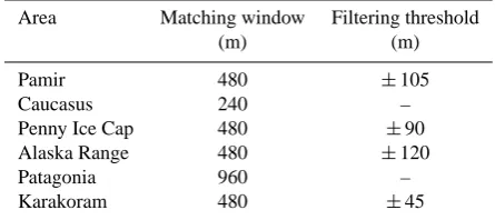
Table 4. Matching window sizes and filtering thresholds in the
dif-ferent areas.
Area Matching window Filtering threshold
(m) (m)
Pamir 480 ±105
Caucasus 240 –
Penny Ice Cap 480 ±90
Alaska Range 480 ±120
Patagonia 960 –
Karakoram 480 ±45
by 17 000 pixels. The size of the small test sections used is 30 km by 30 km. Different window sizes are tested on this section to find a window size that optimizes the match-ing results. The matchmatch-ing result is considered to be opti-mized when assumed correct matches are obtained over most of the glacierized areas, but without increasing the window size more than necessary. This is to avoid much deforma-tion in one window (Debella-Gilo and K¨a¨ab, 2011c). The spacing between the matching windows is half the window size, which means that the matchings are not completely in-dependent. The size of the matching windows used is given in Table 4.
Using specified minimum smoothness of the glacier flow field, we filter the vectors based on comparison with their neighbors. First, all vectors outside glacierized areas are re-moved using digital glacier outlines from GLIMS if available or we digitize such outlines from Landsat images. Using only the remaining vectors, the displacement field in bothx and
y direction is filtered using a 3 by 3 mean low-pass filter. Individual original vectors that deviate more than a certain threshold from this low-pass filtered displacement field are removed (Heid and K¨a¨ab, 2012). The threshold varies be-tween the different areas depending on the displacement vari-ations within the areas. Table 4 shows the different thresh-olds. The low-pass filtered displacement field is only used to
filter the raw displacement field, and not for the final speed comparison. Automatic filtering is not conducted in Cauca-sus and Patagonia because of the few correct matches derived in these areas.
For Pamir, Alaska Range and Karakoram the velocity fields derived are dense enough for comparing velocities de-rived for points closest to the centerline. However, for Cauca-sus, Penny Ice Cap and Patagonia the derived velocity fields are more patchy, and therefore also points further away from the centerline are accepted. In all cases the automatically de-rived results are checked manually by removing points with mismatches in one or both of the two periods. Thus, only points with accepted matches in both periods are used for computing velocity changes.
measurements is ±5 m for ETM+ (Lee et al., 2004) and ±6 m for TM (Storey and Choate, 2004). The accuracy of the matching method is around 1/10 of a pixel (Heid and K¨a¨ab, 2012). We also matched stable ground in all of the image pairs, and for all image pairs the root mean square error (RMSE) was between 1.8 m and 5.7 m. For compari-son of two different displacement measurements, the uncer-tainty will be±8 m for ETM+ and±9 m for TM using root sum square (RSS). Since time spans are about one year, but in some cases slightly shorter, speed changes of more than ±10 m a−1are considered significant speed changes in this study.
We compute the mean speeds and their changes from the means of each individual glacier, not from all measurements directly. This normalization is necessary because some glaciers are large or have good visual contrast and thus allow for many measurements, whereas others do not. However, it is important to notice that the numbers are not area averages since not all glaciers and all parts of glaciers are covered. Deriving glacier velocities using image matching depends on visual contrast in the images. Generally, measurements are therefore restricted to the ablation area and crevassed parts of the accumulation area. Thus, the numbers from our study are indicative for speed changes but do not quantitatively re-flect overall ice flux changes. Decadal reduction in glacier speed is calculated by simply dividing total change through number of decades, not as compound interest due to the short time intervals involved.
3 Results
Changes in glacier speeds are derived for the 2000/2001– 2009/2010 period for Pamir, the 1986/1987–2010/2011 pe-riod for Caucasus, the 1985/1987–2009/2010 pepe-riod for Penny Ice Cap, the 1986/1987–2009/2010 period for Alaska Range, the 1984/1986–2001/2002 period for Patagonia, the 2001/2002–2009/2010 period for Karakoram east, and the 2000/2001–2009/2010 period for Karakoram west. Speed changes from the first to the second period are shown in Figs. 2, 3 and 4 and are also summed up in Table 5. The glacier elevation and the elevation of the measurements in each region are shown in Table 6. Elevation data are ob-tained through http://www.viewfinderpanoramas.org, http:// eros.usgs.gov and http://www.geobase.ca. The largest reduc-tion in speed per decade is found in Pamir where the speed decreased by 43 % per decade. Caucasus has the smallest re-duction in speed of the regions with negative mass balance with only 8 % reduction per decade. Glaciers in Karakoram increased their speeds by 5 % per decade.
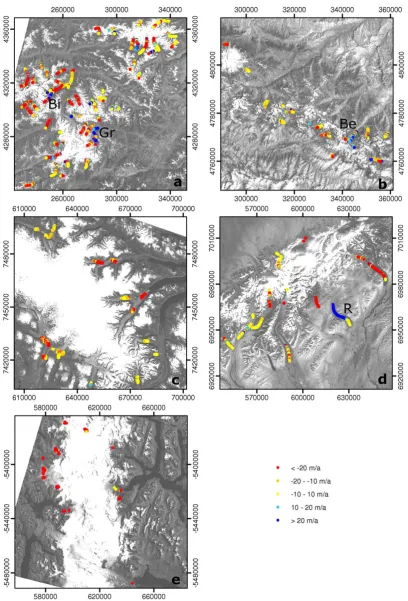
In Pamir we derive speed changes for parts of 50 glaciers. The majority of the glaciers reduced their speed or showed no significant speed changes over the time period, but two glaciers, Bivachnyy and Grum-Grzhimailo, increased their speeds (Fig. 2a). Pamir is a region with surging glaciers
(Dol-gushin et al., 1963), hence also surge activities potentially in-fluence the results. In total the speed decrease is about 39 %, which translates to 43 % per decade.
In Caucasus we derive speed changes for parts of 16 glaciers. Most glaciers reduced their speed over the time pe-riod (Fig. 2b), but the largest glacier in the area, Bezengi glacier, increased its speed over large parts of the glacier. In total, the areas we map show a general decrease in glacier speed of about 19 % over the time period, which translates to about 8 % per decade.
Speed changes are derived for parts of 12 of the outlet glaciers of Penny Ice Cap. Generally all glaciers decreased their speed from the first period to the second (Fig. 2c). The total speed decrease over the areas we map is about 59 %, or 25 % per decade.
The matching in the Alaska Range gives us speed changes for parts of 9 glaciers. All but one glacier, Ruth Glacier, have reduced their speed or had constant speed over the time period (Fig. 2d). Also this is an area with surging glaciers (Post, 1969). In total the speed decrease is about 26 %, or 11 % per decade.
In Patagonia speed changes are derived for 10 of the north-ern outlet glaciers of the Southnorth-ern Patagonia Ice Field. All the outlet glaciers that we map have reduced their speed over the time period (Fig. 2e), and the total percentage of speed reduction is 34 %, or 20 % per decade.
As Fig. 3 shows, the pattern of velocity changes in Karako-ram is complex. In the east, glaciers are mainly increasing their speeds, but the difference in speed between the first and the second period is generally less than 25 m a−1. Two ex-ceptions are Stanghan glacier and Skamri glacier, which have low speeds in the first period and very high speeds in the sec-ond period. In the west, the speed changes are dramatic for glaciers flowing into the Shimshal valley and also for Khiang glacier and Batura glacier. However, there is no clear pattern in the velocity changes, and both accelerating and decelerat-ing glaciers are found. For glaciers in Shimshal valley the speeds are high in both periods, but they are extremely high in one of the periods. Khiang glacier has high speeds in the first period, but in the second period the speed is close to zero. This glacier has not been identified as a surging glacier before. Batura glacier has high speeds in both periods, but the speed is increasing from the first to the second period. A tributary of Batura Glacier in the west is surging in the last period, influencing also the speed of Batura Glacier in the confluence zone. Overall, glaciers in Karakoram increased their speeds with about 5 % per decade, but as Fig. 4 shows, the variation in this area is considerable and the speed change thus not statistically significant.
Fig. 2. Glacier speed changes between the two periods for (a) Pamir, (b) Caucasus, (c) Penny Ice Cap, (d) Alaska Range and (e) Patagonia.
Table 5. Speed change for each area.
Area Mean Mean Percent Percent Number of Number of
speed change speed 1. period speed change speed change points glaciers per decade
(m a−1) (m a−1) decade−1
Pamir −17.0 45.8 −39 % −43 % 3148 50
Caucasus −4.9 25.7 −19 % −8 % 1057 16
Penny Ice Cap −11.3 21.3 −53 % −22 % 471 12
Alaska Range −15.9 61.2 −26 % −11 % 1018 9
Patagonia −85.3 248.6 −34 % −20 % 85 10
Karakoram 1.9 39.3 5 % 5 % 9370 181
Fig. 3. Differences in centerline speed in Karakoram between the two periods 2001–2002 (east)/2000–2001 (west) and 2009–2010. Negative
values indicate lower speeds in the last period. Changes between−10 m a−1 and 10 m a−1are insignificant. Note that the scale is different compared to Fig. 2. The large red circles indicate glaciers that are known to surge (Hewitt, 1969, 2007; Copland et al., 2009). Ba indicates Batura, Bo indicates Baltoro, Sh indicates Shimshal valley, Kh indicates Khiang, Sk indicates Skamri, St indicates Stanghan and Si indicates Siachen.
increase by 4.1 m a−1 from 2000–2001 to 2004–2005, and from 2004–2005 to 2009–2010 they decrease by 18.3 m a−1. Only 1873 points are used to derive the changes using the in-termediate period in Pamir due to striped Landsat-7 images that reduce the number of correct matches. On Penny Ice Cap the speeds increase by 1.5 m a−1from 1985–1987 to 1997– 1998, whereas they decrease by 11.3 m a−1from 1997–1998 to 2009–2010. In this area the same points are being used to derive speed changes using the intermediate period as are being used to derive speed changes without the intermediate period.
4 Discussion
Pamir Caucasus Penny Alaska R. Patagonia Karakoram −200
−150 −100 −50 0 50 100 150
Speed change [m/a]
Fig. 4. The speed change of individual glaciers from the first to the second period for the six different regions. The box outline indicates the
25th percentile and the 75th percentile. The dotted bars indicate the range of the speed changes. Negative values indicate lower speeds in the second period.
Table 6. Elevation of glaciers and speed change measurements in each area.
Area Elevation Elevation Mean elevation Mean elevation glaciers measurements glaciers measurements
(m) (m) (m) (m)
Pamir 2583–7490 2670–5171 4779 4244
Caucasus 1755–5629 1755–3809 3551 2677
Penny Ice Cap 14–2135 218–849 1293 600
Alaska Range 185–6188 237–2286 1755 865
Patagonia 0–3600 215–1432 1317 710
Karakoram 2366–8600 2554–6618 5250 4216
the mass balance changes are taking place. Second, mass balance changes upward of a cross-section propagate down-glacier as kinematic waves (Paterson, 1994). The speed of the kinematic wave is greater than the ice speed, and at the wave front the ice flux changes according to the mass bal-ance. The time it takes for a glacier to adjust its front po-sition, and thereby also its front velocity, to a change in its mass balance is called the response time of glaciers (Johan-nesson et al., 1989). The response time ranges from tens of years for glaciers in warm and wet areas to several thousand years for glaciers in cold and dry climates (Raper and Braith-waite , 2009). However, the reaction time, which is the time it takes before mass balance changes start to effect the termi-nus, can be very rapid.
As Table 6 shows, the speed change measurements are mainly restricted to the lower parts of the glaciers where the visual contrast favors image matching. When the mass bal-ance is negative the ice flux will be reduced over time be-cause there is less mass to transport. This effect accumulates down-glacier so that the change in ice flux is expected to be small in higher areas of the glaciers and high in lower ar-eas of the glaciers. Because our speed change mar-easurements
mainly cover the ablation area they are not representative for entire glaciers, and speed changes for the entire glacierized areas will be lower than what we have estimated here.
(Frapp´e and Clarke, 2007), may have influenced our mea-surements. Fifth and finally, note that our measurements rep-resent speed changes between two annual periods, and not necessarily steady changes in ice flux on a decadal scale.
Seasonal velocity variations with respect to the image ac-quisition dates used potentially influence our findings. Wher-ever possible we therefore tried to find images of a similar point in time within the year. Also, averaging speeds and speed changes over a large number of glaciers will limit the influence of seasonal velocity variations if one assumes that these variations do not happen synchronously over a region. From these considerations follows that the Alaska Range re-sults with the largest difference in acquisition season, in par-ticular between times 1 and 2, and the smallest number of glaciers might potentially be most influenced by velocity sea-sonality.
Some of the glaciers are accelerating from the first to the second period. Both Pamir and the Alaska Range contain surging glaciers. It is therefore not surprising that some glaciers in these areas are accelerating. The Bivachnyy Glacier in Northwestern Pamir is clearly a surge type glacier in its quiescent phase in the first period, due to velocities close to zero. In the second period this glacier is moving much faster with maximum speed of about 100 m a−1. These speeds probably reflect a surge or surge-type movement. Looped moraines on this glacier are visible in the satellite images and confirm that it is a surge-type glacier. The Grum-Grzhimailo Glacier to the southeast in Pamir and the accel-erating glacier in Alaska Range, Ruth Glacier, cannot be de-fined as surge type glaciers from the velocity measurements obtained in this study. These glaciers have speeds of more than 100 m a−1 in both periods, and in addition no looped moraines can be seen in the satellite images. It is however likely that these changes are more related to surge type ac-tivity than to changes in mass balance since the glaciers are situated in areas containing surging glaciers and because they behave differently from their neighboring glaciers. The ac-celerating glacier in Caucasus, Bezengi Glacier, can possibly be accelerating as a reaction to positive mass balance val-ues. Mean mass balance here was close to zero for the period 1966/1967 to 2002/2003 (Shahgedanova et al., 2007), and the mass balance measurements were only done on one glacier, the Djankuat Glacier, so mass balance might have been pos-itive for Bezengi Glacier.
Although Penny Ice Cap and Patagonia have a smaller de-crease in glacier speed per decade than Pamir, these are the two areas that show the most homogeneous speed decrease from the first period to the second. No glacier in these two ar-eas accelerates, and in Patagonia almost all compared points show a speed decrease of more than 20 m a−1from the first to the second period. This is probably because all investi-gated glaciers in these two areas are dynamically stable and hence only have velocity variations that can be attributed to changes in mass balance.
The moderate increase in glacier speeds in Eastern Karakoram indicates that these glaciers are increasing their speeds as a response to the positive mass balance in this area. Quincey et al. (2009a) proposed that Baltoro accelerated due to positive mass balance, and the present study shows that this is also the case for Siachen Glacier. Staghan Glacier and Skamri Glacier are clearly surge-type glaciers in their quies-cent phase in the first period due to their low speeds. In the second period the glaciers are surging according to derived speeds of more than 200 m a−1and also large areas where the speed cannot be measured probably due to very high speeds and much surface transformation.
Many of the glaciers flowing into the Shimshal valley are glaciers with flow instabilities. They cannot be characterized as surge type glaciers from the speed changes derived in this study. This is because they have large speeds in both periods, hence sliding is clearly an important component of the sur-face speed although the velocities are lower than in the other period. A previous study has speculated that many glaciers in the Karakoram have flow instabilities instead of being of classical surge type (Williams and Ferrigno, 2010). The re-sults in the present study for glaciers flowing into Shimshal valley support this.
The velocity measurements obtained here indicate that glaciers in Karakoram behave differently depending on lo-cation. Glaciers in the east (around Siachen and Baltoro) seem to be dynamically stable and their speed changes are linked to changes in mass balance. This is also supported by the very few observations of glacier surges in this area, and few looped moraines. The Central North Karakoram (around Skamri) probably contains many surging glaciers because of the very low speeds that are measured in this area. This indi-cates that these are surging glaciers in their quiescent phase. Many of these glaciers have also been identified as surging glaciers in previous studies (Hewitt, 1969, 2007; Copland et al., 2009). The area in northwest (around Shimshal) con-tains many glaciers that vary their speeds considerably be-tween the two periods. However many of them cannot be defined as surging glaciers in the classical sense. This is be-cause the speed is high in both periods, and therefore sliding seems very important at all times. This area also contains some classical surging glaciers.
5 Conclusions and perspectives
On regional scales and over longer time periods, the glacier speeds are expected to decrease because less mass accumu-lates and therefore also less mass will be transported down to lower elevations. We have shown that this regional speed de-crease is taking place. We did not have the data to investigate whether there is a quantitative relationship between the mag-nitude of the negative mass balance and the percent speed de-crease. This is because the response time of glaciers is differ-ent from area to area, and within the areas, and due to other reasons such as the uncertain representativeness of our ve-locity measurements with respect to available mass balance data. Glaciers in Karakoram generally increased their speed due to the positive mass balance, but the speed changes here are heavily influenced by the dynamic instabilities.
Our study opens up for a range of other analyses based on regional or worldwide glacier velocity measurements as were demonstrated here. For instance, it seems possible to roughly estimate the response time of glaciers from inventory param-eters (Haeberli and Hoelzle, 1995), and investigate their cor-relation with speed changes and mass balance measurements. Velocity measurements can be correlated against glacier in-ventory parameters such as length, area and hypsometry. Glacier velocities can also be used to estimate erosion rates or mechanisms (Scherler et al., 2011b) and transport times (Casey et al., 2012) and thus to contribute towards better un-derstanding of glacial landscape development. On the more applied side, widespread decrease in glacier speed will in-crease the probability and speed of glacier lake development in areas prone to such lakes, because ice supply is one of the dominant factors in lake development and growth. Studies of speed change can help to point out areas where glacier lakes can develop or the growth of existing ones is expected (K¨a¨ab et al., 2005a; Bolch et al., 2008; Quincey et al., 2007).
As a future glacier monitoring strategy, annual velocities should be derived every year, preferably for all glaciated re-gions of the world. Such a monitoring of glacier veloci-ties would allow to study worldwide changes in the veloc-ity fields. Doing this every year would also enable to track significant year-to-year speed variations, which are missed in our study due to the longer time periods between the velocity fields derived.
Now that recent studies have demonstrated that it is fea-sible not just to focus velocity measurements on specific glaciers or smaller glacier regions, more effort should be put into deriving glacier velocities globally. This study shows that deriving glacier velocities for large regions or even on a global scale can give valuable insights to glaciers’ dynamic climate change response and to glacier flow instabilities. It also shows that there is a potential to understand the impor-tance of glacier sliding and deformation on regional scales better by investigating speed changes over time and the spa-tial structure of velocities.
Supplementary material related to this
article is available online at: http://www.the-cryosphere. net/6/467/2012/tc-6-467-2012-supplement.zip.
Acknowledgements. Glacier outlines are downloaded from the GLIMS database http://glims.colorado.edu/glacierdata/. Landsat images are downloaded from http://glovis.usgs.gov/. Elevation data are obtained through http://www.viewfinderpanoramas.org, http://eros.usgs.gov and http://www.geobase.ca. We received valuable comments on the manuscript by Duncan Quincey, an anonymous referee, Mauri Pelto, Ian Howat, Luke Copland and Christopher Nuth. The study is funded by The Research Council of Norway through the Precise analysis of mass move-ments through correlation of repeat images (CORRIA) project (no. 185906/V30), the ESA Climate Change Initiative project Glaciers cci (4000101778/10/I-AM), and the International Centre for Geohazards (SFF-ICG 146035/420). The study is also a contribution to the “Monitoring Earth surface changes from space” study by the Keck Institute for Space Studies at Caltech/JPL.
Edited by: I. M. Howat
References
Bahr, D., Dyurgerov, M., and Meier, M.: Sea-level rise from glaciers and ice caps: a lower bound, Geophys. Res. Lett., 36, L03501, doi:10.1029/2008GL036309, 2009.
Bernstein, R.: Image geometry and rectification, in: Manual of Remote Sensing, American Society of Photogrammetry, Falls Church, VA, 881–884, 1983.
Berthier, E., Vadon, H., Baratoux, D., Arnaud, Y., Vincent, C., Feigl, K., Remy, F., and Legresy, B.: Surface motion of moun-tain glaciers derived from satellite optical imagery, Remote Sens. Environ., 95, 14–28, doi:10.1016/j.rse.2004.11.005, 2005. Berthier, E., Schiefer, E., Clarke, G. K. C., Menounos, B.,
and Remy, F.: Contribution of Alaskan glaciers to sea-level rise derived from satellite imagery, Nature Geosci., 3, 92–95, doi:10.1038/NGEO737, 2010.
Bindschadler, R. and Scambos, T.: Satellite-image-derived veoloc-ity field of an Antarctic ice stream, Science, 252, 242–246, 1991. Bishop, M., Olsenholler, J., Shroder, J., Barry, R., Raup, B., Bush, A., Copland, L., Dwyer, J., Fountain, A., Haeberli, W., K¨a¨ab, A., Paul, F., Hall, D. K., Molnia, J. K., Trabant, D., and Wessels, R.: Global land ice measurements from space (GLIMS): remote sensing and GIS investigations of the Earth’s cryosphere, Geocarto International, 19, 57–85, 2004.
Bolch, T., Buchroithner, M. F., Peters, J., Baessler, M., and Ba-jracharya, S.: Identification of glacier motion and potentially dangerous glacial lakes in the Mt. Everest region/Nepal using spaceborne imagery, Nat. Hazards Earth Syst. Sci., 8, 1329– 1340, doi:10.5194/nhess-8-1329-2008, 2008.
Casey, K. A., K¨a¨ab, A., and Benn, D. I.: Geochemical characteriza-tion of supraglacial debris via in situ and optical remote sens-ing methods: a case study in Khumbu Himalaya, Nepal, The Cryosphere, 6, 85–100, doi:10.5194/tc-6-85-2012, 2012. Copland, L., Pope, S., Bishop, M., Schroder Jr., J. F., Clendon, P.,
ve-locities across the Central Karakoram, Ann. Glaciol., 50, 41–49, 2009.
Copland, L, Sylvestre, T., Bishop, M. P., Shroder, J. F., Seong, Y. B., Owen, L. A., Bush, A., and Kamb, U.: Expanded and recently increased glacier surging in the Karakoram, Arct. Antarct. Alp. Res., 43, 503–516, 2011.
Debella-Gilo, M. and K¨a¨ab, A.: Sub-pixel precision algorithms for normalized cross-correlation based image matching of mass movements, Remote Sens. Environ., 115, 130–142, 2011a. Debella-Gilo, M. and K¨a¨ab, A.: Monitoring slow-moving
land-slides using spatially adaptive least squares image matching, in: Proceedings of the Second World Landslide Forum, 3–9 Oct 2011, Rome, Italy, 2011b.
Debella-Gilo, M. and K¨a¨ab, A.: Locally adaptive template sizes for matching repeat images of Earth surface mass move-ments, ISPRS J. Photogramm. Remote Sens., 69, 10–28, doi:10.1016/j.isprsjprs.2012.02.002, 2012.
Dolgushin, L. D., Yevteyev, S. A., Krenke, A. N., Rototayev, K. G., and Svatkov, N. M.: The recent advance of the Medvezhiy glacier, Priroda II, 85–92, 1963.
Fitch, A. J., Kadyrov, A., Christmas, W. J., and Kittler, J.: Orienta-tion correlaOrienta-tion, in: British Machine Vision Conference, Cardiff, UK, 2–5 September 2002, 133–142, 2002.
Frapp´e, T.-P. and Clarke, G.: Slow surge of Trapridge Glacier, Yukon territory, Canada, J. Geophys. Res.-Earth, 112, F03S32, doi:10.1029/2006JF000607, 2007.
Gardner, A., Moholdt, G., Wouters, B., Wolken, G., Burgess, D., Sharp, M., Cogley, J., Braun, C., and Labine, C.: Sharply increased mass loss from glaciers and ice caps in the Canadian Arctic Archipelago, Nature, 473, 357–360, doi:10.1038/nature10089, 2011.
Haeberli, W. and Hoelzle, M.: Application of inventory data for estimating characteristics of and regional climate-change effects on mountain glaciers: a pilot study with the European Alps, Ann. Glaciol., 21, 206–212, 1995.
Haefeli, R.: Changes in the behaviour of the Unteraargletscher in the last 125 years, J. Glaciol., 9, 195–212, 1970.
Haug, T., K¨a¨ab, A., and Skvarca, P.: Monitoring ice shelf velocities from repeat MODIS and Landsat data - a method study on the Larsen C ice shelf, Antarctic Peninsula, and 10 other ice shelves around Antarctica, The Cryosphere, 4, 161–178, doi:10.5194/tc-4-161-2010, 2010.
Heid, T. and K¨a¨ab, A.: Evaluation of existing image matching meth-ods for deriving glacier surface displacements globally from op-tical satellite imagery, Remote Sens. Environ., 118, 339–355, 10.1016/j.rse.2011.11.024, 2012.
Herman, F., Anderson, B., and Leprince, S.: Mountain glacier ve-locity variation during a retreat/advance cycle quantified using sub-pixel analysis of ASTER images, J. Glaciol., 57, 197–207, 2011.
Hewitt, K.: Glacier surges in Karakoram Himalaya (Central Asia), Can. J. Earth Sci., 6, 1009–1018, 1969.
Hewitt, K.: The Karakoram Anomaly? Glacier Expansion and the “Elevation Effect”, Karakoram Himalaya, Mountain Research and Development, 25, 332–340, doi:10.1659/0276-4741(2005)025[0332:TKAGEA]2.0.CO;2, 2005.
Hewitt, K.: Tributary glacier surges: an exceptional concentration at Panmah Glacier, Karakoram Himalaya, J. Glaciol., 53, 181– 188, doi:10.3189/172756507782202829, 2007.
Johannesson, T., Raymond, C., and Waddington, E.: Time-scale for adjustment of glaciers to changes in mass balance, J. Glaciol., 35, 355–369, 1989.
Kargel, J., Abrams, M., Bishop, M., Bush, A., Hamilton, G., Jiskoot, H., K¨a¨ab, A., Kieffer, H., Lee, E., Paul, F., Rau, F., Raup, B., Shroder, J., Soltesz, D., Stainforth, D., Stearns, L., and Wessels, R.: Multispectral imaging contributions to global land ice measurements from space, Remote Sens. Environ., 99, 187–219, doi:10.1016/j.rse.2005.07.004, 2005.
K¨aser, G., Cogley, J. G., Dyurgerov, M. B., Meier, M. F., and Ohmura, A.: Mass balance of glaciers and ice caps: Consen-sus estimates for 1961–2004, Geophys. Res. Lett., 33, L19501, doi:10.1029/2006GL027511, 2006.
Kaufmann, V. and Ladst¨adter, R.: Quantitative analysis of rock glacier creep by means of digital photogrammetry using multi-temporal aerial photographs: two case studies in the Austrian Alps, Permafrost, 1/2, 525–530, 2003.
K¨a¨ab, A.: Monitoring high-mountain terrain deformation from re-peated air- and spaceborne optical data: examples using digital aerial imagery and ASTER data, ISPRS J. Photogramm. Remote Sens., 57, 39–52, 2002.
K¨a¨ab, A.: Combination of SRTM3 and repeat ASTER data for deriving alpine glacier flow velocities in the Bhutan Himalaya, Remote Sens. Environ., 94, 463–474, doi:10.1016/j.rse.2004.11.003, 2005.
K¨a¨ab, A., Huggel, C., Fischer, L., Guex, S., Paul, F., Roer, I., Salz-mann, N., Schlaefli, S., Schmutz, K., Schneider, D., Strozzi, T., and Weidmann, Y.: Remote sensing of glacier- and permafrost-related hazards in high mountains: an overview, Nat. Hazards Earth Syst. Sci., 5, 527–554, doi:10.5194/nhess-5-527-2005, 2005a.
K¨a¨ab, A., Lefauconnier, B., and Melvold, K.: Flow field of Kro-nebreen, Svalbard, using repeated Landsat 7 and ASTER data, Ann. Glaciol., 42, 7–13, 2005b.
Lee, D., Storey, J., Choate, M., and Hayes, R.: Four years of Landsat-7 on-orbit geometric calibration and per-formance, IEEE T. Geosci. Remote, 42, 2786–2795, doi:10.1109/TGRS.2004.836769, 2004.
Lemke, P., Ren, J., Alley, R., Allison, I., Carrasco, J., Flato, G., Fujii, Y., K¨aser, G., Mote, P., Thomas, R., and Zhang, T.: Ob-servations: changes in snow, ice and frozen ground, in: Climate Change 2007: The physical science basis. Contribution of Work-ing Group I to the Fourth Assessment Report of the Intergov-ernmental Panel on Climate Change, edited by: Solomon, S., Qin, D., Manning, M., Chen, Z., Marquis, M., Averyt, K. B., Tignor, M., and Miller, H. L., Cambridge University Press, Cam-bridge, UK and New York, NY, USA, 2007.
Leprince, S., Barbot, S., Ayoub, F., and Avouac, J.: Automatic and precise orthorectification, coregistration, and subpixel cor-relation of satellite images, application to ground deforma-tion measurements, IEEE T. Geosci. Remote, 45, 1529–1558, doi:10.1109/TGRS.2006.888937, 2007.
Lucchitta, B. and Ferguson, H.: Antarctica – measuring glacier ve-locity from satellite images, Science, 234, 1105–1108, 1986. McFadden, E. M., Howat, I. M., Joughin, I., Smith, B. E., and
Ahn, Y.: Changes in the dynamics of marine terminating outlet glaciers in west Greenland (2000–2009), J. Geophys. Res., 116, F02022, 10.1029/2010JF001757, 2011.
Ox-ford, 1994.
Post, A.: Distribution of surging glaciers in western North America, J. Glaciol., 8, 229–240, 1969.
Quincey, D. J. and Glasser, N. F.: Morphological and ice-dynamical changes on the Tasman Glacier, New Zealand, 1990–2007, Global Planet. Change, 68, 185–197, doi:10.1016/j.gloplacha.2009.05.003, 2009.
Quincey, D. J., Richardson, S. D., Luckman, A., Lucas, R. M., Reynolds, J. M., Hambrey, M. J., and Glasser, N. F.: Early recognition of glacial lake hazards in the Himalaya using re-mote sensing datasets, Global Planet. Change, 56, 137–152, doi:10.1016/j.gloplacha.2006.07.013, 2007.
Quincey, D. J., Copland, L., Mayer, C., Bishop, M., Luckman, A., and Belo, M.: Ice velocity and climate variations for Baltoro Glacier, Pakistan, J. Glaciol., 55, 1061–1071, 2009a.
Quincey, D. J., Luckman, A., and Benn, D.: Quantification of Ever-est region glacier velocities between 1992 and 2002, using satel-lite radar interferometry and feature tracking, J. Glaciol., 55, 596–606, 2009b.
Quincey, D. J., Braun, M., Glasser, N. F., Bishop, M. P., Hewitt, K., and Luckman, A.: Karakoram glacier surge dynamics, Geophys. Res. Lett., 38, L18504, doi:10.1029/2011GL049004, 2011. Raper, S. C. B. and Braithwaite, R. J.: Glacier volume response
time and its links to climate and topography based on a concep-tual model of glacier hypsometry, The Cryosphere, 3, 183–194, doi:10.5194/tc-3-183-2009, 2009.
Raup, B., K¨a¨ab, A., Kargel, J., Bishop, M., Hamilton, G., Lee, E., Paul, F., Rau, F., Soltesz, D., Khalsa, S., Beedle, M., and Helm, C.: Remote sensing and GIS technology in the global land ice measurements from space (GLIMS) project, Comput. Geosci., 33, 104–125, doi:10.1016/j.cageo.2006.05.015, 2007. Rignot, E., Rivera, A., and Casassa, G.: Contribution of the
Patag-onia Icefields of South America to sea level rise, Science, 302, 434–437, doi:10.1126/science.1087393, 2003.
Rolstad, C., Amlien, J., Hagen, J. O., and Lund´en, B.: Visible and near-infrared digital images for determination of ice velocities and surface elevation during a surge on Osbornebreen, a tidewa-ter glacier in Svalbard, Ann. Glaciol., 24, 255–261, 1997. Scambos, T. A., Dutkiewicz, M. J., Wilson, J. C., and
Bind-schadler, R. A.: Application of image cross-correlation to the measurement of glacier velocity using satellite image data, Re-mote Sens. Environ., 42, 177–186, 1992.
Scherler, D., Leprince, S., and Strecker, M. R.: Glacier-surface ve-locities in alpine terrain from optical satellite imagery – accu-racy improvement and quality assessment, Remote Sens. Envi-ron., 112, 3806–3819, 2008.
Scherler, D., Bookhagen, B., and Strecker, M. R.: Spatially variable response of Himalayan glaciers to climate change affected by de-bris cover, Nature Geosci., 4, 156–159, doi:10.1038/ngeo1068, 2011a.
Scherler, D., Bookhagen, B., and Strecker, M. R.: Hillslope-glacier coupling: the interplay of topography and glacial dy-namics in High Asia, J. Geophys. Res.-Earth, 116, F02019, doi:10.1029/2010JF001751, 2011b.
Shahgedanova, M., Popovnin, V., Petrakov, D., and Stokes, C. R.: Long-term change, interannual and intra-seasonal variabil-ity in climate and glacier mass balance in the Central Greater Caucasus, Russia, Ann. Glaciol., 46, 355–361, doi:10.3189/172756407782871323, 2007.
Skvarca, P., Raup, B., and De Angelis, H.: Recent behaviour of Glaciar Upsala, a fast-flowing calving glacier in Lago Argentino, Southern Patagonia, Ann. Glaciol., 36, 184–188, 2003.
Span, N. and Kuhn, M.: Simulating annual glacier flow with a linear reservoir model, J. Geophys. Res., 108, 4313, doi:10.1029/2002JD002828, 2003.
Storey, J. and Choate, M.: Landsat-5 bumper-mode geomet-ric correction, IEEE T. Geosci. Remote, 42, 2695–2703, doi:10.1109/TGRS.2004.836390, 2004.
Vincent, C., Vallon, M., Reynaud, L., and Le Meur, E.: Dy-namic behaviour analysis of glacier de Saint Sorlin, France, from 40 years of observations, 1957–97, J. Glaciol., 46, 499–506, doi:10.3189/172756500781833052, 2000.
Vincent, C., Soruco, A., Six, D., and Le Meur, E.: Glacier thick-ening and decay analysis from 50 years of glaciological obser-vations performed on Glacier d’Argentiere, Mont Blanc area, France, Ann. Glaciol., 50, 73–79, 2009.
WGMS: Glacier Mass Balance Bulletin No. 5 (1996–1997), edited by: Haeberli, W., Hoelzle, M., and Frauenfelder, R., IAHS (ICSI)/UNEP/UNESCO. World Glacier Monitoring Service, Zurich, Switzerland, 96 pp., 1999.
WGMS: Global Glacier Change: Facts and Figures, edited by: Zemp, M., Roer, I., K¨a¨ab, A., Hoelzle, M., Paul, F., and Hae-berli, W., UNEP, World Glacier Monitoring Service, Zurich, Switzerland, 88 pp., 2009.