M E T H O D O L O G Y
Open Access
Discovering feature relevancy and
dependency by kernel-guided probabilistic
model-building evolution
Nestor Rodriguez and Sergio Rojas–Galeano
**Correspondence: [email protected] Universidad Distrital FJC, School of Engineering, Bogota, Colombia
Abstract
Background: Discovering relevant features (biomarkers) that discriminate etiologies of a disease is useful to provide biomedical researchers with candidate targets for further laboratory experimentation while saving costs; dependencies among biomarkers may suggest additional valuable information, for example, to characterize complex epistatic relationships from genetic data. The use of classifiers to guide the search for biomarkers (the so–calledwrapperapproach) has been widely studied. However, simultaneously searching for relevancy and dependencies among markers is a less explored ground. Results: We propose a new wrapper method that builds upon the discrimination power of a weighted kernel classifier to guide the search for a probabilistic model of simultaneous marginal and interacting effects. The feasibility of the method was evaluated in three empirical studies. The first one assessed its ability to discover complex epistatic effects on a large–scale testbed of generated human genetic problems; the method succeeded in 4 out of 5 of these problems while providing more accurate and expressive results than a baseline technique that also considers dependencies. The second study evaluated the performance of the method in benchmark classification tasks; in average the prediction accuracy was comparable to two other baseline techniques whilst finding smaller subsets of relevant features. The last study was aimed at discovering relevancy/dependency in a hepatitis dataset; in this regard, evidence recently reported in medical literature corroborated our findings. As a byproduct, the method was implemented and made freely available as a toolbox of software components deployed within an existing visual data–mining workbench. Conclusions: The mining advantages exhibited by the method come at the expense of a higher computational complexity, posing interesting algorithmic challenges regarding its applicability to large–scale datasets. Extending the probabilistic
assumptions of the method to continuous distributions and higher–degree interactions is also appealing. As a final remark, we advocate broadening the use of visual graphical software tools as they enable biodata researchers to focus on experiment design, visualisation and data analysis rather than on refining their scripting programming skills.
Keywords: Relevancy discovery, Dependency estimation, Feature selection, Epistasis, Hepatitis dataset, Visual programming tools
Background
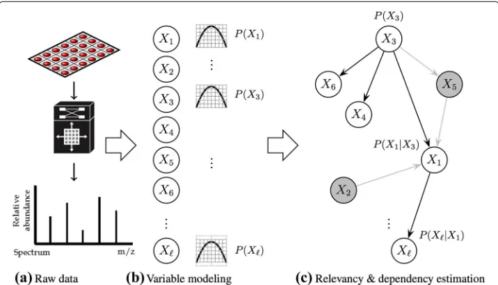
The current state of data acquisition technology is providing industry and academy with large–scale sources of information that are relatively cheap to store and collect, but expen-sive to process and understand; this phenomenon is pervaexpen-sive to domains as diverse as bioinformatics, fraud detection, computer vision, recommender systems, particle physics, financial analysis, weather forecasting, and social networks media streaming, to name a few. One of the main challenges arising in processing such huge amounts of data, is to discover from the many observed variables (also known asfeatures), those that are most relevant to explain significant patterns –or markers– of hidden concepts. This task is known as feature selection in the data–mining community or biomarker discovery in the biomedical ambit. In addition to relevancy discovery, also of interest is the identifica-tion of interacidentifica-tions (dependencies) between those markers; a schematic depicidentifica-tion of such relevancy–dependency scenario is illustrated in Fig. 1.
Relevancy estimation techniques are aimed at finding subsets of markers in datasets with a high number of dimensions, where noisy, redundant or irrelevant variables abound. The selected features may become targets of more detailed studies requiring expensive experimentation or human expertise, thus saving costs and time not spent on the dis-carded variables. This problem of selecting the relevant variables can be regarded as a search procedure over the space of all possible combinations of variable subsets, therefore, an NP-Hard problem [1]; similarly, finding the underlying structure of a graph represent-ing dependencies between those variables is also combinatorial [2]. Thus the need of usrepresent-ing approximating, iterative methods is an alternative to find suitable solutions.
Research in techniques for discovering relevant variables is a very active field in the data mining community (see e.g. [2–7]), and has attracted much attention in the last two decades [8]. Thefilterapproach ranks the variables according to a linear criterion such as
their correlation to the prediction target; they are computational simple, but usually fails to capture non–linear patterns of discrimination.
In contrast, the wrapperapproach performs the search guided by the classification accuracy of a discriminant rule that evaluates the suitability of a subset of features; although computationally more demanding, this setting is able to find smaller and more discriminative sets of relevant features, specially when non–linear concepts are hid-den. In this respect several approaches have been proposed previously using different metaheuristics, probabilistic assumptions and discrimination techniques. One particular flavor uses probabilistic model–building genetic algorithms combined with well–known classifiers (a review of applications of this approach in the bioinformatics domain can be found in [9]). This kind of algorithms simultaneously estimate the parameters of a probabilistic relevance model of the variables andthe structure of a graph represent-ing relationships among them. Recent studies usrepresent-ing a Bayes network as such model have reported promising results in discovering interactions in genetic data [2, 6, 10, 11].
In a similar vein, here we describe a novel method that models relevancy and depen-dency by coupling a weighted kernel machine for pattern classification [12] into a probabilistic–based genetic algorithm [13] for dependency estimation. Previous studies considered combining classical and probabilistic genetic algorithms with weighted ker-nel classifiers for relevancy–only discovery [14, 15]; our contribution in this paper is to extend those approaches to take advantage of the discrimination power of a weighted ker-nel classifier to guide the search for a probabilistic model that simultaneously estimates marginal and interacting effects among the features in a discrimination problem.
Method Previous work
Overview of probabilistic-based genetic algorithms
This kind of genetic algorithms are stochastic search techniques that evolve a probability distribution model from a pool of solution candidates, rather than evolving the pool itself. The distribution is adjusted iteratively with the most promising (sub-optimal) solutions until convergence. Hence, they are also known as Estimation of Distribution Algorithms (EDA, for short). The generic estimation procedure is shown in Algorithm 1. Step (1) initialises the model parametersθ. Step (2) is the loop that updates the parametersθuntil convergence. Step (3) samples a poolS ofncandidates from the model. Step (4) ranks the pool according to a cost functionf(·)and chooses the top-ranked into B. Step (5) re-estimates the parametersθ from this subset of promising solutions.
Algorithm 1:Generic EDA
Input: Pool sizen, problem dimensionality, and cost functionf(·)
1 θ ←initialize()
2 repeatuntilθ converges
3 S←sample(P(X;θ),n)
4 B←select(S,f(·)) 5 θ ←estimate(θ,B)
6 end
The actual realisation of each step in the generic template of Algorithm 1 defines differ-ent types ofEDAs: discrete or continuous parameters; binomial, multinomial or Gaussian distributions; univariate, bivariate or multivariate dependencies, see among others: [14, 16–23]. Our approach to the problem of interest is based on the following assump-tions: discrete parameters, Gaussian distributions, bivariate dependencies.
For this purpose we resorted to build upon the Bivariate Marginal Estimation of Distribution Algorithm (BMDA) proposed by [19]. InBMDA the nodes of a graphG are associated to the problem variablesXi, and pair-wise dependencies are represented with a minimum-spanning-forest,MSF(see Fig. 2). The roots of theMSFcorrespond to indepen-dent variables associated with marginal effects, whereas the rest of the nodes correspond to dependant variables associated to interaction effects with respect to their parents (notice that in a forest, any non–root node has at most one parent). Therefore, the prob-ability model assumed by BMDA is the following bivariate binomial distribution with parametersθ = {MSF,{ρi},{ρij}}, whereRMSFis the set of root variables,EMSFis the set of
interactions among the variables, and{ρi}and{ρij}are the parameters of the independent and interacting factors respectively, of the overall probability distribution:
P(X;θ)= i∈RMSF
P(Xi;ρi)
(i,j)∈EMSF
P(Xi|Xj;ρj,ρij)
BMDA adheres to the generic EDA template of Algorithm 1, with tailored sampling and estimation rules that we describe next for illustration purposes. Firstly, the sampling mechanism (Step (3) in the algorithm) is modified as to preserve the most promising can-didatesBfrom the previous iteration along with new candidates sampled from the current model (n2candidates):
S=sampleP(X;θ),n 2
∪B (1)
Secondly, the estimation strategy (Step (5) in the algorithm) comprises the following operations:
1. Build adisconnected graphG(V,Et), withVthe set of problem variables, andEt the set of variable interactions determined by a bivariate Pearsonχ2dependency test criterion:Et= {(i,j)∈V×V:i=j∧χij2≥3.84}. Here the statisticχ2is computed from the current candidate poolBat iterationt.
2. ComputeMSF(Et)representing variable dependencies. Build the set of root nodes
RMSFby choosing at random one node of every component inMSF(Et).
3. Estimate parameters{ρi:i∈RMSF}and{ρij:(i,j)∈EMSF}using frequentist
updates (see Eq. (2)), again over the current candidate poolBat iterationt(N.B. Here,[c]=1if the argumentcis true or 0 otherwise).
ρa i =
n
k=1
[Bki=a] , ρijab= n
k=1
Bki=a∧Bkj=b
, (2)
Overview of kernel machines for pattern classification
As it was mentioned earlier, we use a classifier that guides the search for more suitable subsets of features (Step 4 of Algorithm 1). From the many pattern classification tech-niques, kernel machines [12] have shown outstanding performance on diverse problem domains; thus we chose them as base classifiers for our method.
Kernel machines classify patterns using a linear combination of nonlinear mappings, known as kernel functions, evaluated on the current input instanceiover the observed instances in the pastj < i, using the ruleyˆi = sign
i−1
j=1αjκ(xj,xi)
, where ˆyi is the class prediction and the coefficients{αj} are learnt with standard linear discriminant algorithms such as thePerceptronor theSVM[12].
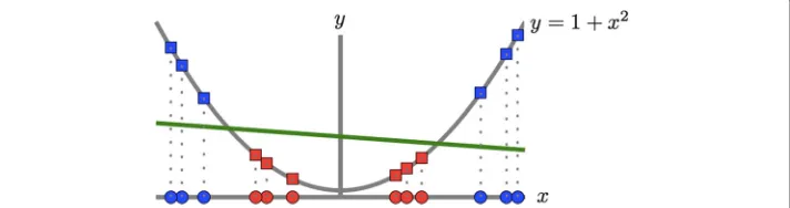
The classification power of kernel machines is partly due to the ability of the kernel function to map the input space into a higher–dimensional space [24], that is,κ(xj,xi)=
(xj)(xi). In such transformed space nonlinearities are probably easier to resolve, while the classifier preserves the computational simplicity of a linear discriminant in input space [25] (see Fig. 3). There is no need to explicitly declare the nonlinear mapping as long as the kernel function is defined as a symmetric positive semidefinite function [12, 24]. Two of such widely–used kernel functions are the RBF and the polynomial ker-nel,κσ(x,z)=exp−σi=1(xi−zi)2
, andκd(x,z)=(xz)d. The parametersσandd define the width of the RBF and the degree of the polynomial kernel, respectively.
Modified weighted versions of these kernels incorporate scale factorsw= {w1,. . .,w: wi∈[0, 1]}for each of thedimensions (i.e. variables) in order to modulate their contri-bution to the total computation [14, 26, 27]. The weighted RBF and weighted polynomial kernels are then defined asκσ(x,z;w) = exp−σi=1wi(xi−zi)2
, andκd(x,z;w) =
i=1wi(xi·zi)
d
, respectively. Here we remark that aswiis closer to 1, its associated variable becomes more relevant since it contributes a larger magnitude to the final value of the kernel computation. It is in this sense that we interpret the vectorwas representing
Fig. 3Transforming the input space onto a higher dimensional space using a nonlinear mapping(·), may resolve nonlinearities with linear discriminants. Here a binary dataset (positive class=red, negative=blue) is visualised in two different subspaces, a line inR1and a parabola inR2. The original data (ovals) is not linearly
separable inR1. The transformed data (squares) is separable inR2by an arbitrary linear discriminant (green).
the relevancy distribution of the variables for the purposes of classification. Accordingly, classification performance will guide theEDAto estimate these relevancy factors.
Additionally we observe that because of the additive nature of these kernel functions, the resulting scaling in each dimension can be obtained by preprocessing the input data with a modified version of the weight vectorw. For instance, regarding the RBF kernel it can be seen that:
κσ(x,z;w)=exp −σ
i=1
wi(xi−zi)2
=exp −σ
i=1 √
wixi−√wizi
2
=κσ(w⊗x,w⊗z),
wherew= {√w1,. . .,√w}and⊗denotes the component–wise product. The case of the
weighted polynomial kernel is analogous. This observation was originally pointed out in [14] and more recently in [27].
Related methods for relevancy and dependency estimation
Some previous studies have considered a multi-objective approach for simultaneous opti-misation of accuracy and relevance distribution. Two representative techniques utilise
EDAs to estimate the parameters of a probability model from which the relevance fac-tors are sampled. One of such approaches, theEBNAalgorithm [28]) uses a multivariate probabilistic model that incorporates second–order dependencies between the variables. The search of relevancy and dependencies is guided by the discriminatory power of a Naive-Bayes classifier. The authors report promising results in finding suitable variable subsets with good generalisation performance, although the benefit of obtaining insights about relationships between variables is traded–off with an overhead in computational complexity.
On the other hand,wKierais a wrapper approach for feature relevance estimation that combinesEDAs and kernel machines [14]. The estimation is carried out using an array of scale factors coupled to a weighted kernel machine whose classification accuracy guides the search for the relevance distribution using an UMDA algorithm [13]. The authors reported encouraging results compared to filter methods in discovering relevant variables on a number of different classification tasks, including problems with linear and non-linear hidden concepts in very–high dimensional spaces. The algorithm however, does not retrieve additional information about the interactions between the relevant variables, because it assumes they are conditionally independent. In this respect, wKiera dif-fers from the method we propose in this paper which, despite combining also a kernel machine with anEDA, estimates relevance based on a probabilistic model of bivariate interactions, obtaining a network of dependencies that may provide additional insights regarding the combined effects of related features, as we shall explain in the next section.
The scores computed byReliefFare positive for relevant features and negative for irrelevant ones. Although it does not provide explicit information about the dependen-cies, this technique has proven fast and effective for relevance estimation on problems with strong feature interactions, where other filters become myopic and fail to find them [30].
Proposed algorithm
The new method that we termedweigthed Kernel Iterative Estimation of Dependencies and Relevancy Algorithm (Kiedrafor short) uses a hybridised version of BMDA and
wKierato estimate the relevancy distribution and second order dependencies of input variables. The search is guided by the suitability of the relevance factors when classifying the data with its corresponding weighted kernelSVM. The following steps were introduced in the design ofKiedra:
• When building the correlation graph, the Mutual Information (MI) criterion [31] was additionally considered to estimate dependencies between arbitrary pairs of variables, that is, to the extent to which they share information. A third Combined Mutual Information andp-value (SIM) criterion was also considered; the latter mixes both statistical and information–theory dependence [32]. Consequently, the rule to compute the edges on the dependency network was modified to that in Eq. (3):
Et=
(i,j)∈V×V:i=j∧any_of
χ2
ij ≥3.84,MIij>0,SIMij>0
(3)
• When choosing the root nodesRMSFof the dependency network (forest), instead of
selecting at random we introduced another information–theory criterion that selects nodes minimising the marginal entropyH(·)in each connected componentVkof the network,kVk=V ∧ kVk = ∅, as stated in Eq. (4). The marginal entropy is computed frequentist-wise from the current candidate poolBat iterationt. The rationale behind the introduction of this criterion is that those nodes with lowest entropy are richer in information content, and thus good candidates to become independent parents of the dependency subnetworks (in this sense this criterion was originally proposed in theMIMICalgorithm [17]).
RMSF=
rk:rk =arg min i
H(Xi∈Vk)
(4)
• Finally, candidate relevance factors are sampled from the current probability model and incorporated to a population including the previous best solutions found: S ←sample(P(X;θ),n2)∪B. Each candidate in this populationwk∈Sis assessed by building a weightedSVMand obtaining its classification accuracy with a 5–fold cross–validation on the modified datasetD←D⊗wk. The population is ranked by best accuracies and the top candidates are selected. These candidates are then used to re–estimate the dependency network and the relevance parameters of the
Empirical study
In this section we report the results of a number of experiments designed to validate the feasibility of the proposed method. Initially we provide details about our implemen-tation platform. Then we describe the first experiment aimed at testing the ability of the method in discovering epistasis on generated human genetic datasets; there we used
ReliefFas a baseline to compare, for it is also a method that treats feature interactions. Our empirical study continued with a second experiment designed to compare the pro-posed approach with otherEDA-based and kernel-based methods on some benchmark classification problems. Lastly, we conducted a third experiment intended again to dis-cover relevancy and dependencies in a medical domain, specifically on a hepatitis dataset, this time corroborating the results with recent findings in the literature of that disease.
Implementation
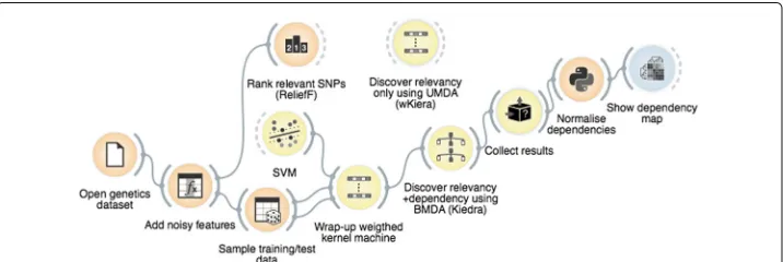
The method was implemented using theGoldenberrysuite of visual components for stochastic–based search optimisation within theOrangemulti–platform workbench for data mining [33, 34]. In this environment, visual components (known aswidgets) exe-cuting different steps of the algorithm such as data input and sampling,SVMs training,
BMDAestimation, etc., are dragged onto a visual canvas where they are assembled to cre-ate theKiedraprogram shown in Fig. 4. TheWrapperCostFunctionwidget is the core of the program; it gets input from theDataandSVMwidgets and wraps them up in a weighted kernel machine which in turn is provided as the cost function required by theBMDAoptimiser. Additional widgets were used for comparison withReliefFand
wKiera, and also for results collection and visualisation, namelyRank,DistanceMap,
BlackBoxTesterandUMDA(we note in passing that thewKieraalgorithm can be implemented by simply replacingBMDAwithUMDAin this assemblage). More information of these widgets and their configuration can be found in the Additional file 1: Additional Methods and Tools section.
Experiment 1: Relevancy and dependency in genetic epistasis
Genetic epistasis refers to those complex gene-gene interactions that may trigger sus-ceptibility to a common human disease. Instead of characterising a single nucleotide
polymorphism (SNP) as an isolated marker of a disease, epistasis assumes a combi-nation of markers is in fact associated to the phenotypic manifestation of the disease. Hence, epistasis in genetic datasets is an interesting target for simultaneous relevance and dependencies mining.
In this first set of experiments we focused on evaluating the effectiveness of the method in discovering such complex interactions. For this purpose we considered a recently proposed testbed of human genetic–like model–free datasets simulating eti-ologies between combinations of SNPs [35]; the datasets were designed to minimise predictiveness of single or pairs of genetic variations and maximise highe–order inter-actions. The original datasets consisted of 3, 4 or 5 SNPs; we modified them by adding both 5 and 10 features unrelated to disease status so as to represent three, four, or five-way epistatic problems polluted with noise. The irrelevant features were sampled from an uniform random distribution as Ri ∼ U(0, 10). A summarised description of these datasets is given in Table 1; those labeled as “NoLow” indicates that no lower– effects can be found, that is, epistasis involves strong interactions among the entire set of relevant SNPs. Besides, we chose ReliefF as a baseline to compare the perfor-mance of the proposed method, considering its ability to also treat feature interactions, is well-known [30].
For each dataset, the experiment was conducted following the scheme shown in Fig. 4. On the one hand, once the noise was added, features in the polluted dataset were scored usingReliefF; those obtaining positive scores were labeled as relevant, otherwise as irrelevant. On the other hand,Kiedraexperiments were executed as follows. Firstly the modified dataset was split in training and testing subsets (25%/75%); then anSVMwas parameterised (C=100, RBF kernel withσ =10) and wrapped–up in a weighted kernel machine along with the data. The latter was then provided as the cost function to evolve a BMDA (n= 20,iter= 80, SIM criterion). In view of the stochastic nature ofKiedra, the above protocol was repeated 30 times with the resulting scale factors being collected and averaged; then a cut–off threshold of 0.7 was applied to select relevant from irrelevant features.
The subsets found with both methods were finally contrasted to the ground truth in order to record a coordinate(#R, #N)of the correct number of relevant(#R)and noisy
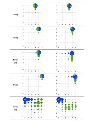
(#N) features that were discovered. These records are summarised in the bubble fre-quency plots of Fig. 5. They are arranged according to their pollution rate (5 or 10 added noisy features). Here, the area of any bubble in each problem represent the frequency at which the method hit the corresponding coordinate(#R, #N) of relevant and noisy features within the 100 datasets.
Let us examine first the plots in the left-hand column of the figure. In the first two prob-lems,3wayand4way,Kiedrawas able to discover the correct number of relevant and
Table 1Description of simulated epistatic problems (see [35] for further details)
Problem Datasets Simulated SNPs Noisy SNPs Disease status Instances
3way 100 3 5 and 10 0 or 1 3000 (balanced) 4way 100 4 5 and 10 0 or 1 3000 (balanced) 4way-NL 100 4 5 and 10 0 or 1 3000 (balanced) 5way 100 5 5 and 10 0 or 1 3000 (balanced)
Fig. 5Bubble frequency plot of epistasis discovery withKiedra(blue) andReliefF(green). Plots are arranged by epistatic problem in rows, i.e. number of relevant SNPs, and noise pollution in columns, i.e. number of irrelevant features: 5 (left) or 10 (right). One hundred datasets per problem were analysed; a bubble in any plot depicts the relative frequency of correct discovered (#relevant, #noisy) features
corresponding to its coordinate (abscissas are #relevant). Largest bubbles are the most frequent result found byKiedrain each problem; the slices shown in such bubbles illustrate in proportion (hits) how often ReliefFagreed with that finding
noisy features within the whole collection of datasets. Likewise, in problems4way-NL
and5way, Kiedraonly missed a few 2 datasets in each problem.ReliefFin turn, discovered correctly up to 84, 97 and 93 datasets in problems3way,4wayand5way, achieving a lower rate of 61 hits for problem4way-NL. These results hint at the abil-ity ofKiedrato discover epistatic effects even with coexisting uninformative markers.
Now, let us discuss the results shown in the plots of the right–hand column of the figure. We recall that these problems were modified with twice the number of polluted features. A similar trend can be seen for the behaviour ofKiedra. The method achieved a correct hit rate of 98 out of 100 in problems3wayand4way; this rate was down to 80 in problem4way-NLand slightly lower in5way. On the other hand,ReliefFwas adversely affected by such level of noise, for it obtained correct hit rates of 44, 39, 3 and 12 respectively.
Finally, let us comment on the plots of the last row in the figure (problem
5way-NL), whose results differ amply from those reported previously. In this prob-lem, ReliefFseems to perform better in comparison withKiedra, although not a conclusive trend is evident. In the 5-noisy features problem it is able to find the cor-rect coordinate (5,5) in about 10 hits, but the most frequent result was coordinate (4,4) with 21 datasets. Likewise in the 10-noisy features problem the most frequent discov-ered coordinate was (3,5) while the optimal (5,10) was never found. On the other hand,
Kiedra clearly underperformed in this problem as their findings are highly biased to coordinates where the correct number of noisy features are identified, but in contrast few or none of the relevant are found. We recall that the originators of these epistatic datasets reckon that this is the hardest problem, as its etiology comprises interactions of the entire set of 5 SNPs, while no lower-degree interactions were enabled, as opposed to the other problems [35]. We remark however, that the dependency graph in whichKiedrais based assumes a bi–variate probability distribution, which may explain why it fails in modeling higher–order interactions appropriately.
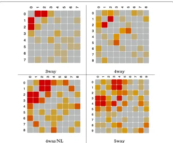
On a different note, it is worth mentioning that at the expense of obtaining explicit information about gene–gene interactions,Kiedrais computationally more demand-ing thanReliefF. This is becauseKiedrarequires training and testing a classifier at every iteration during the evolution of its probability model. This effort is compensated however, by its ability to explicitly compute the feature dependency graph while searching for the relevant variables. To illustrate this point, Fig. 6 shows examples of dependency heatmaps generated from the dependency graph computed byKiedrafor arbitrary cho-sen datasets belonging to problems3wayto 5way(5 noisy features), whose epistasis, as it was discussed above, was correctly discovered by the method. These dependency heatmaps are symmetric matrices that were visualised using theShowDependencyMap
widget of Fig. 4. Notice that each interaction map is meant to be interpreted jointly with the associated relevance factors, in order to identify informative interactions between rel-evant features and to ignore irrelrel-evant interactions. For example, in the shown heatmaps the epistatic interactions would be located in the section of the matrices involving fea-tures 0 to 2 (3way) or 0 to 3 (4way) or 0 to 4 (5way), as those were the features correctly selected as relevant byKiedra. In contrast, one can argue that the remainder sections of the matrices contain spurious dependencies arising from correlations due to randomness of the added noise, a fact corroborated because these features were correctly designated as irrelevant by the method.
Experiment 2: Feature relevance discovery in benchmark classification problems
Fig. 6Dependency heat maps in epistatic problems with 5 added noisy features. These matrices represent dependency graphs (gene–gene interactions) computed byKiedra(notice that dependencies are non–directed since matrices are symmetric). Relevant variables are numbered starting from 0 (i.e. {0,1,2} in problem3way, {0,1,2,3} in problem4wayand so on). Interaction intensity is represented by a warm–based gradient palette
from the UCI repository [36] (see description in Table 2). The results forEBNAwere taken from those reported in [28]. wKieraandKiedrawere implemented with the visual components of Fig. 4.
One experiment was conducted per each dataset as follows. The dataset was initially preprocessed as to fill–in missing values with a Naive Bayes classifier and to normalise within a [0, 1] real interval. The processed dataset was then randomly split intotraining andtestsubsets of equal size. These subsets are the inputs for the cross–validation scheme used to estimate the accuracy of each candidate solution. For each method, 10 repetitions were executed with different random splits. Average statistics were collected using the
BlackBoxTesterwidget.
We evaluated the performance of these methods in two aspects: relevancy discovery and classification accuracy. Firstly, let us examine the average number of relevant variables
Table 2Description of benchmark classification datasets
Dataset Variables Classes Instances
Ionosphere 34 2 351
Soybean 35 19 307
Horse–colic 27 24 368
Annealing 38 6 798
Table 3Average number of relevant variables discovered in each dataset
Dataset Raw EBNA wKiera Kiedra
Ionosphere 34 13.40±2.11 7.30±0.82 7.20±0.92
Soybean 35 6.10±1.85 5.10±0.99 6.50±1.58 Horse–colic 27 18.90±2.76 16.40±1.90 16.60±2.12 Annealing 38 20.50±3.13 9.60±0.97 9.40±1.43 Image 19 8.00±0.66 7.72±1.24 7.45±1.36
per dataset, which are reported in Table 3. It is clear thatKiedraandwKierashow comparable results; besides both obtained smaller variable subsets than those ofEBNA.
Kiedrawas able to outperformwKierain three cases. Reduction rates in the number of variables with respect to the original dimensionality, varied from around 76% or more (Ionosphere, Soybean and Annealing) to 60% (Image) to 40%, (Horse–colic). It is worth noting that in two cases (Ionosphere and Annealing), the new method achieved around half the size of the subsets found withEBNA; moreover, these were among the datasets with higher number of raw variables.
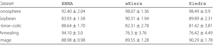
Regarding average classification accuracy (see Table 4), againKiedraandwKiera
show similar performance, with a slight advantage toKiedrain two datasets. The sim-ilarity in the performance of these two techniques was anticipated, given that both are based on a kernel classifier (SVM). However, we remark thatKiedraprovides additional valuable information about possible dependencies in the variable subsets, whichwKiera
do not. On the other hand,EBNAoutperformed the kernel-based techniques in two cases (Horse–colic and Annealing), suggesting the Naive Bayes classifier may yield more effec-tive discriminants for those datasets, although using larger feature subsets (almost twice the size).
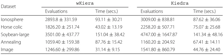
Lastly, we also report on runtime performance statistics for the kernel–based methods (see Table 5). In average,wKieraneeded fewer evaluations of the cost function in order to converge, compared toKiedra; in terms of execution times there is no conclusive evi-dence of one method being faster that the other. However, we reckon these differences as being not remarkable, considering thatKiedrasimultaneously produces estimates about possible variable dependencies. Unfortunately runtime information was not reported in the referencedEBNAreport.
Experiment 3: Relevancy and dependency estimation on a medical domain
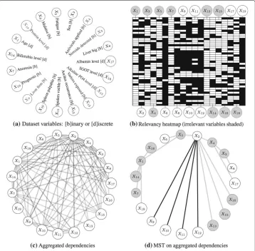
The third study was focused on assessing the simultanoeus relevancy/dependency ability of the method on a medical domain. It was conducted on theHepatitisdataset from the UCI repository [36, 37]. In this dataset, 19 clinical observations from 155 patients suf-fering from hepatitis were recorded, along with the final outcome (die or survive). The notation and domain of the variables in the dataset are given in Fig. 7(a).
Table 4Average prediction accuracy in each dataset
Dataset EBNA wKiera Kiedra
Ionosphere 92.40±2.04 98.07±1.36 98.49±0.9 Soybean 83.93±1.58 90.31±1.94 89.89±2.31 Horse–colic 88.64±1.70 82.31±2.78 81.42±3.81 Annealing 94.10±3.0 76.3±3.76 76.42±4.49
Table 5Average runtime performance (only available forwKieraandKiedra)
Dataset wKiera Kiedra
Evaluations Time (secs.) Evaluations Time (secs.)
Ionosphere 2893.8±331.59 93.11±30.21 3009.00±838.81 87.62±36.06
Horse colic 1826.20±251.74 43.02±13.19 2258.20±507.71 75.07±25.68 Soybean-large 3501.00±437.77 151.04±38.42 4747.00±1647.87 141.34±48.16 Annealing 1059.40±159.38 87.76±15.42 1160.20±204.92 67.41±14.11 Image 1246.60±299.86 31.14±9.15 1541.80±860.79 44.76±24.40
The experiment was implemented using the sameKiedratestbed of Fig. 4; we simply changed the data source. The data was preprocessed and sampled for training and test-ing subsets as before. This protocol was repeated 100 times in order to prevent biased results due to randomness in the proposed method. Relevancy factors of the best solu-tion found in each repetisolu-tion were collected; then, variables discovered in more than half of the repetitions yielding accuracies greater than 80%, were selected as relevant (see the relevancy heatmap of Fig. 7(b)).
Additional variability was induced by shuffling the order of the patients in the dataset in each repetition. As a result we noticed dissimilar dependency trees were found. Thus, these trees were aggregated into a single graph, accounting the strengths of the dependen-cies as proportional to the number of times they showed up during the repetitions (see Fig. 7(c)). Lastly, in order to estimate the final pairwise dependencies, we computed the minimum-spanning-treeon this aggregated graph, using the inverse of the counts as edge costs and applying Kruskal’s algorithm [38] (see Fig. 7(d)).
Kiedrafound a total of nine relevant variables: Sex (X2), Malaise (X6), Liver big (X8),
Liver firm (X9), Spleen palpable (X10), Spiders visible (X11), Ascites occurrence (X12),
Albumin level (X17) and Prognosis (X19). Besides, according to Fig. 7(b), the method found
strong evidence of relevancy in subset{X6,X19}, followed by fair evidence of relevancy
in {X8,X9,X10,X11,X12}, and lastly, borderline evidence in {X2,X17}. The first subset
indicates, not surprisingly, that prognosis by histology is probably the most effective pre-dictor of the disease, although being expensive and risky of complications [39]; similarly, malaise is seemingly correlative with the disease and it is a symptom usually reported by patients [40].
In contrast, the second subset correspond to more disease-specific symptoms: hep-atomegaly (liver oversizing and stiffness) and splenomegaly (spleen enlargement) com-monly reflect severity of liver damage [39, 41], spider nevi are visible in patients with the different variants of the disease [42, 43], and ascites has been reported as being strongly associated with hepatic dysfunctions [44]. Regarding the last subset, albumin is a protein synthesised in the liver, so it is reasonable to correlate changes in its level with infection with hepatitis. The peculiar finding here is Sex (X2), a non-disease-specific variable that
nonetheless, has been recently linked to treatment response and survival rates with other unexpected features such as race (female, white) [39, 44]. In addition, it is worth noting that the relevant dependencies found by our method are between this variable and the other disease-specificX9,X10,X11,X12predictors mentioned earlier.
We remark that these findings are corroborated by other related studies, such as [45] suggesting that variables X19, X11, X17 and X12 were highly indicative of the
Fig. 7Relevancy and dependency discovery in theHepatitisdataset usingKiedra(see the discussion of these results in the text).aDescription of the variables in the dataset.bA heatmap of the discovered relevancy factors; each row correspond to the factors comprising the best solution of one repetition of the experiment. Relevant (white) and irrelevant (shaded) variables where chosen with a cutoff value of 0.5 on the average factors over all repetitions (only repetitions obtaining a classification accuracy greater than 80% were considered).cA graph of aggregated dependencies obtained over all repetitions. Opacity indicates the frequency of repetition a dependency was found.dThe minimum-spanning-tree on the aggregated graph, suggesting the final estimated dependencies. Relevancy is also shown (irrelevant variables and associated dependencies are shaded)
{X6,X17,X14,X19,X11}as relevant, with further experimentation finding predictive value
in variableX2. Other studies using information theoretic, statistical and regularisation
learning methods [47] as well as various machine learning and bioinspired techniques [48] also reported these variables in their relevant subsets, or report subsets with similar sizes (10–12 variables) obtaining similar prediction accuracies between 80–85% [49].
On the other hand, the following variables were characterised as not explanatory by
Kiedra: Age (X1), Steroids detected (X3), Antivirals applied (X4), Fatigue (X5), Anorexia
(X7), Varices exposed (X13), Bilirrubin level (X14), Alkaline PO4 level (X15), SGOT level
(X16) and Protein level (X18). From this subset, it causes surprise bilirrubin not being
dataset such information was not available. The other potential marker included in this subset is the alkaline phosphate level; however, some clinical studies have shown that this enzyme maintain normal levels during hepatitis infection, although it may raise in other hepatic–related injuries such as cholestasis [40].
No further evidence of other data mining studies assigning relevancy in the remainder variables was found [37, 47, 48]. Notice that consequently, we also regarded the depen-dencies associated with these variables as not relevant for the prediction of the disease outcome.
Conclusion
We have described a method to tackle the dual combinatorial problem of relevancy-dependency discovery by coupling a weighted kernel classifier to guide the evolution of a probabilistic model of marginal and interacting effects among the problem features. Empirical evidence found in two experiments, one in a genetic epistasis testbed and another in a classification benchmark, indicates comparable performance with related baseline methods while providing richer dependency and relevancy information; in a third experiment comprising a hepatitis dataset, the method findings were corroborated with those reported in recent medical literature.
The promising potential mining capabilities of the method come at the expense of higher computational complexity of the algorithmic and data structures that it involves. In view of the nowadays increasingly availability of high–throughput and stream technolo-gies for data acquisition, natural questions emerge in regards to the applicability of the method in large–scale scenarios. In this respect, we envisage two interesting avenues for further research, the first one related to algorithmic crafting so as to speed up the compu-tation of the kernel function, which might be a bottleneck in such big data scenarios e.g. [14, 27, 50, 51]; the second one is considering compact representations of the probability model enabling memory and time savings during updating of its parameters [23, 52–54]. On a different perspective, the current design of the method is restricted to discrete probabilistic models; therefore modeling continuous distributions with its associated computational challenges, is also of significant interest. Besides, since the probabilistic model assumes a bivariate distribution, the method is prone to miss epistasis due to higher–order interactions, as it was shown in the hardest genetic problem in the empirical study. Thus, future work would also consider addressing this limitation.
As a final word, we also advocate adopting user–friendly visual graphical data–mining tools enabling biomedical analysts to focus on their experiments rather than on improving their low–level programming skills (see [55] for deeper insights on visual programming environments for bioinformatics). Hence, an additional challenge arising is growing and refining the suite of visual software components that currently implements the method.
Additional file
Additional file 1:Additional Methods and Tools. (PDF 153 kb)
Acknowledgements Not applicable.
Availability of data and materials
The epistatic human-like gentic datasets are available at: https://github.com/greenelab/model-free-data (last visit: December 08/2016). The benchmark classifications and hepatitis datasets are available in the UC Irvine Machine Learning Repository (available at: http://archive.ics.uci.edu/ml/, last visit: December 08/2016). The software used for
experimentation in this article is publicly available as:
Project name: Goldenberry. (http://goldenberry-labs.org, last visit: December 08/2016). Version: 2.0
Operating systems: Platform independent Programming language: Python, Qt Other requirements: Orange version 2.7 License: Simplified BSD License
Authors’ contributions
SRG conceived the problem and the hybrid dependency–relevancy method, designed the study, interpreted the results, and led the drafting of the manuscript. NR developed the software used to implement the method, conducted the experiments, collected the results, and helped interpreting the results. All authors read and approved the final manuscript.
Authors’ information
NR contribution was done while he was a graduate student at Universidad Distrital FJC, School of Engineering.
Competing interests
The authors declare that they have no competing interests.
Consent for publication Not applicable.
Ethics approval and consent to participate Not applicable.
Received: 5 August 2016 Accepted: 14 February 2017
References
1. Davies S, Russell S. NP-completeness of searches for smallest possible feature sets. In: AAAI Symposium on Intelligent Relevance. Palo Alto: AAAI Press; 1994. p. 37–9.
2. Gheisari S, Meybodi MR, Dehghan M, Ebadzadeh MM. Bayesian network structure training based on a game of learning automata. Intl J Mach Learn Cybernet. 2016;Online first:1–13.
3. Aldehim G, Wang W. Determining appropriate approaches for using data in feature selection. Intl J Mach Learn Cybernet. 2016;Online first:1–14.
4. Bolón-Canedo V, Sánchez-Maroño N, Alonso-Betanzos A, Benítez JM, Herrera F. A review of microarray datasets and applied feature selection methods. Inf Sci. 2014;282(0):111–35.
5. Szymczak S, Holzinger E, Dasgupta A, Malley JD, Molloy AM, Mills JL, Brody LC, Stambolian D, Bailey-Wilson JE. r2vim: A new variable selection method for random forests in genome-wide association studies. BioData Mining. 2016;9(1):1–15.
6. Li J, Malley JD, Andrew AS, Karagas MR, Moore JH. Detecting gene-gene interactions using a permutation-based random forest method. BioData Mining. 2016;9(1):1–17.
7. Taguchi Y-H. Principal component analysis based unsupervised feature extraction applied to budding yeast temporally periodic gene expression. BioData Mining. 2016;9(1):1–23.
8. Guyon I, Nikravesh M, Gunn S, Zadeh LA. Feature Extraction: Foundations and Applications. Berlin Heidelberg: Springer; 2006.
9. Armañanzas R, Inza I, Santana R, Saeys Y, Flores JL, Lozano JA, Peer Y. V. d., Blanco R, Robles V, Bielza C, Larrañaga P. A review of estimation of distribution algorithms in bioinformatics. BioData Mining. 2008;1(1):1–12. 10. Su C, Andrew A, Karagas MR, Borsuk ME. Using bayesian networks to discover relations between genes,
environment, and disease. BioData Mining. 2013;6(1):1–21.
11. Motsinger-Reif AA, Deodhar S, Winham SJ, Hardison NE. Grammatical evolution decision trees for detecting gene-gene interactions. BioData Mining. 2010;3(1):1–15.
12. Shawe-Taylor J, Cristianini N. Kernel Methods for Pattern Analysis. New York: Cambridge University Press; 2004. 13. Larrañaga P, Lozano JA. Estimation of Distribution Algorithms: A New Tool for Evolutionary Computation. Boston:
Kluwer Academic Publishers; 2002.
14. Rojas-Galeano S, Hsieh E, Agranoff D, Krishna S, Fernandez-Reyes D. Estimation of relevant variables on high-dimensional biological patterns using iterated weighted kernel functions. PLoS ONE. 2008;3(3):1806. 15. Rojas S, Fernandez-Reyes D. Adapting multiple kernel parameters for support vector machines using genetic
algorithms. In: Proceedings of the 2005 IEEE Congress on Evolutionary Computation. Edinburgh: IEEE; 2005. 16. Muhlenbein H, Paag G. From recombination of genes to the estimation of distributions: I. binary parameters In:
Voigt H-M, Ebeling W, Rechenberg I, Schwefel H-P, editors. Parallel Problem Solving from Nature PPSN IV. Lecture Notes in Computer Science. Berlin Heidelberg: Springer; 1996. p. 178–87.
18. Sebag M, Ducoulombier A. Extending population-based incremental learning to continuous search spaces. In: International Conference on Parallel Problem Solving from Nature. Springer; 1998. p. 418–427.
19. Pelikan M, Müehlenbein H. The bivariate marginal distribution algorithm In: Roy R, Furuhashi T, Chawdhry P, editors. Advances in Soft Computing. London: Springer; 1999. p. 521–35.
20. Larrañaga P, Etxeberria R, Lozano JA, Peña JM. Combinatorial optimization by learning and simulation of bayesian networks. In: Proceedings of the Sixteenth Conference on Uncertainty in Artificial Intelligence. Burlington: Morgan Kaufmann; 2000. p. 343–52.
21. Pelikan M, Goldberg DE. Hierarchical bayesian optimization algorithm = bayesian optimization algorithm + niching + local structures. Burlington: Morgan Kaufmann; 2001. p. 525–32.
22. Nakao M, Hiroyasu T, Miki M, Yokouchi H, Yoshimi M. Real-coded estimation of distribution algorithm by using probabilistic models with multiple learning rates. Procedia Comput Sci. 2011;4:1244–51.
23. Neri F, Iacca G, Mininno E. Compact optimization. In: Handbook of Optimization. Berlin Heidelberg: Springer; 2013. p. 337–64.
24. Aizerman MA, Braverman EA, Rozonoer L. Theoretical foundations of the potential function method in pattern recognition learning. Autom Remote Control. 1964;25:821–37.
25. Cortes C, Vapnik V. Support-vector networks. Mach Learn. 1995;20:273–97.
26. Chapelle O, Vapnik V, Bousquet O, Mukherjee S. Choosing multiple parameters for Support Vector Machines. Mach Learn. 2002;46:131–59.
27. Tan M, Tsang IW, Wang L. Towards ultrahigh dimensional feature selection for big data. J Mach Learn Res. 2014;15(1):1371–429.
28. Inza I, Larrañaga P, Etxeberria R, Sierra B. Feature subset selection by bayesian network-based optimization. Artif Intell. 2000;123(1–2):157–84.
29. Kononenko I, Šimec E, Robnik-Šikonja M. Overcoming the myopia of inductive learning algorithms with relieff. Applied Intell. 1997;7(1):39–55. doi:10.1023/A:1008280620621.
30. Robnik-Šikonja M, Kononenko I. Theoretical and empirical analysis of relieff and rrelieff. Mach Learn. 2003;53(1-2):23–69.
31. Peng H, Long F, Ding C. Feature selection based on mutual information: criteria of max-dependency, max-relevance, and min-redundancy. IEEE Trans Pattern Anal Mach Intell. 2005;27:1226–38.
32. Perlich C, Rosset S. Identifying bundles of product options using mutual information clustering. In: SDM. Philadelphia: SIAM; 2007. p. 390–7.
33. Demšar J, Curk T, Erjavec A, Hoˇcevar T, Milutinoviˇc M, Možina M, Polajnar M, Toplak M, Stariˇc A, Štajdohar M, Umek L, Žagar L, Žbontar J, Žitnik M, Zupan B. Orange: Data mining toolbox in python. J Mach Learn Res. 2013;14:2349–353.
34. Garzón-Rodriguez LP, Diosa HA, Rojas-Galeano S. Deconstructing GAs into Visual Software Components. In: Proceedings of the Companion Publication of the 2015 on Genetic and Evolutionary Computation Conference. GECCO Companion ’15. New York: ACM; 2015. p. 1125–32.
35. Himmelstein DS, Greene CS, Moore JH. Evolving hard problems: Generating human genetics datasets with a complex etiology. BioData Mining. 2011;4(1):21.
36. Bache K, Lichman M. The UCI repository of Machine Learning databases. 2013.
37. Diaconis P, Efron B. Computer intensive methods in statistics. Sci Am. 1983;248(5):116–31.
38. Cormen TH, Leiserson CE, Rivest RL, Stein C. Introduction to Algorithms, 3rd edn. Cambridge: MIT Press; 2009. 39. Rosen HR. Chronic hepatitis C infection. N Engl J Med. 2011;364(25):2429–38.
40. Ryder S, Beckingham I. ABC of diseases of liver, pancreas, and biliary system: acute hepatitis. BMJ Br Med J. 2001;322(7279):151.
41. Kuroda H, Kakisaka K, Oikawa T, Onodera M, Miyamoto Y, Sawara K, Endo R, Suzuki K, Takikawa Y. Liver stiffness measured by acoustic radiation force impulse elastography reflects the severity of liver damage and prognosis in patients with acute liver failure. Hepatology Res. 2015;45(5):571–7.
42. Younis I, Sarwar S, Butt Z, Tanveer S, Qaadir A, Jadoon NA. Clinical characteristics, predictors, and survival among patients with hepatopulmonary syndrome. Ann Hepatol. 2015;1(14):354—360.
43. Chakradhar G, Sudheer D, Rajeswari G, Sriram K, Siva J, Kumar L, Reddy S. Study of pentoxifylline role on prognosis in patients with acute alcoholic hepatitis. J Evol Med Dental Sci. 2015;4(07):1098–1111.
44. Bernal W, Lee WM, Wendon J, Larsen FS, Williams R. Acute liver failure: A curable disease by 2024? J Hepatol. 2015;62(1):112–20.
45. Breiman L. Statistical modeling: the two cultures (with comments and a rejoinder by the author). Stat Sci. 2001;16(3):199–231.
46. Tuv E, Borisov A, Runger G, Torkkola K. Feature selection with ensembles, artificial variables, and redundancy elimination. J Mach Learn Res. 2009;10:1341–66.
47. Tsanas A, Little M, McSharry P. A methodology for the analysis of medical data. In: Handbook of Systems and Complexity in Health. New York: Springer; 2013. p. 113–25.
48. Subbulakshmi CV, Deepa SN. Medical dataset classification: A machine learning paradigm integrating particle swarm optimization with extreme learning machine classifier. Sci World J. 2015;2015:1–12.
49. Yildirim P. Filter based feature selection methods for prediction of risks in hepatitis disease. Int J Mach Learn Comput. 2015;5(4):258.
50. Herbster M. Learning additive models online with fast evaluating kernels. In: Proceedings of the 14th Annual Conference on Computational Learning Theory and and 5th European Conference on Computational Learning Theory. COLT ’01/EuroCOLT ’01. London: Springer; 2001. p. 444–60.
51. Maji S, Berg A, Malik J. Efficient classification for additive kernel SVMs. Pattern Anal Mach Intell IEEE Trans. 2013;35(1):66–77.
53. Iturriaga S, Nesmachnow S. Solving very large optimization problems (up to one billion variables) with a parallel evolutionary algorithm in CPU and GPU. In: Seventh International Conference on P2P, Parallel, Grid, Cloud and Internet Computing. Victoria: IEEE; 2012. p. 267–72.
54. Dong W, Chen T, Tino P, Yao X. Scaling up estimation of distribution algorithms for continuous optimization. Evol Comput IEEE Trans. 2013;17(6):797–822.
55. Milicchio F, Rose R, Bian J, Min J, Prosperi M. Visual programming for next-generation sequencing data analytics. BioData Mining. 2016;9(1):1–17.
• We accept pre-submission inquiries
• Our selector tool helps you to find the most relevant journal
• We provide round the clock customer support
• Convenient online submission
• Thorough peer review
• Inclusion in PubMed and all major indexing services
• Maximum visibility for your research
Submit your manuscript at www.biomedcentral.com/submit

![Table 1 Description of simulated epistatic problems (see [35] for further details)](https://thumb-us.123doks.com/thumbv2/123dok_us/354353.1527995/9.595.120.479.659.735/table-description-simulated-epistatic-problems-details.webp)