Extracting a low-dimensional description of multiple gene expression datasets reveals a potential driver for tumor-associated stroma in ovarian cancer

M E T H O D

Open Access

Extracting a low-dimensional description of

multiple gene expression datasets reveals a

potential driver for tumor-associated

stroma in ovarian cancer

Safiye Celik

, Benjamin A. Logsdon

, Stephanie Battle

, Charles W. Drescher

, Mara Rendi

, R. David Hawkins

and Su-In Lee

Abstract

Patterns in expression data conserved across multiple independent disease studies are likely to represent important molecular events underlying the disease. We present the INSPIRE method to infer modules of co-expressed genes and the dependencies among the modules from multiple expression datasets that may contain different sets of genes. We show that INSPIRE infers more accurate models than existing methods to extract low-dimensional representation of expression data. We demonstrate that applying INSPIRE to nine ovarian cancer datasets leads to a new marker and potential driver of tumor-associated stroma,HOPX, followed by experimental validation. The implementation of INSPIRE is available at http://inspire.cs.washington.edu.

Keywords:Gene expression, Variable discrepancy, Low-dimensional representation, Module, Conditional dependence, Latent variable,HOPX, Tumor-associated stroma

Background

As datasets increase in size, scope, and generality, the possibility to infer potentially relevant and robust fea-tures from data increases. Extracting a biologically intui-tive low-dimensional representation (LDR) of data in an unsupervised fashion (i.e. based on the underlying struc-ture in the data, not with respect to a particular predic-tion task) has become an important step to identify robust and relevant information from data. Development of unsupervised LDR learning methods is a very active area of modern research in machine learning and high dimensional data analysis [1–3]. Specific machine learning domains to see noted success recently in-clude the development of deep learning algorithms [3], where authors demonstrate enormous increases in performance on difficult tasks such as image and text

classification [4, 5]. Analogously, in cancer transcripto-mics, unsupervised LDR learning has seen success on very difficult problems, such as predicting patient outcome in breast cancer in the DREAM7 breast cancer prognosis challenge [6]. The winning team leveraged an unsuper-vised LDR extraction method on independent transcrip-tomic data from multiple cancer types and significantly outperformed the other contestants in the challenge by a large margin [7] along with all other known prognostic signatures in breast cancer.

There are three main challenges with applying existing unsupervised LDR learning approaches to cancer transcriptomic data. First, any one study may not be generalizable in that there will be either technical (e.g. sample ascertainment) or experimental (e.g. batch effects) confounders that make an LDR of data extracted from an individual dataset in a naïve way not necessarily generalizable to other datasets. Second, identifying simple modules (co-expressed sets of genes) using methods such as WGCNA [8] or simple clustering approaches [9, 10] will not necessarily capture complex dependence struc-tures among the modules. Appropriately accounting for

* Correspondence:[email protected] 1

Department of Computer Science & Engineering, University of Washington, Seattle, WA, USA

3_{Department of Genome Sciences, University of Washington, Seattle, WA,}

USA

Full list of author information is available at the end of the article

rich dependencies among these modules will improve their biological coherence. It has been shown that modeling the dependencies among modules improves the quality of the inferred modules from gene expres-sion data [11]. Finally, and most importantly, most cancer transcriptomic data are within the p≫n re-gime (high-dimensional), i.e. we usually have tens of thousands of genes, but only hundreds of samples at most. This means that a successful method must include a very aggressive dimensionality reduction mechanism that allows generalization across datasets, since the potential for overfitting is high. This implies that models that allow for arbitrarily rich dependen-cies among variables (such as those used in deep learning methods) cannot necessarily be applied with-out overfitting the data.

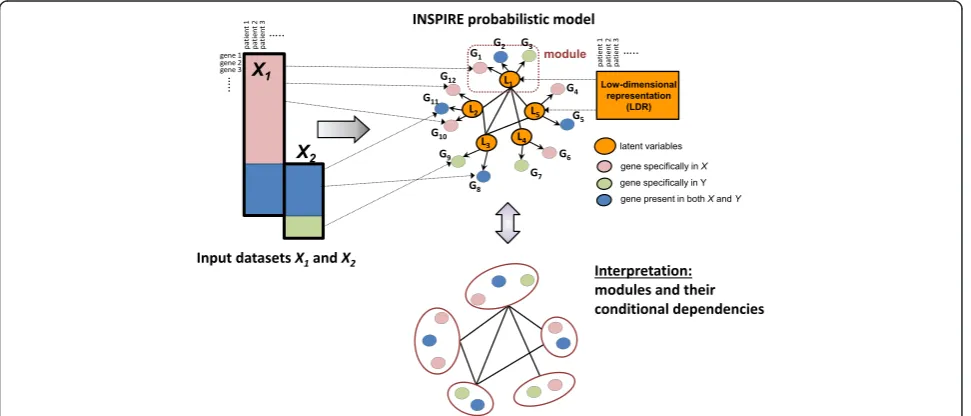
We present a novel unsupervised LDR learning method, called INSPIRE (INferring Shared modules from multiPle gene expREssion datasets), to infer highly coherent and robust modules of genes and their dependencies on the basis of gene expression datasets from multiple independ-ent studies (Fig. 1). INSPIRE is an unconvindepend-entional and ag-gressive data dimensionality reduction approach that extracts highly biologically relevant and coherent modules from gene expression data, where the number of samples is much less than the number of observed genes – the

norm for cancer expression data. INSPIRE addresses the three aforementioned challenges. First, INSPIRE naturally integrates many datasets by modeling the latent (hidden, unobserved) variables in a probabilistic graphical model [12], where the latent variables are modeled as a Gaussian graphical model, which is the most commonly used prob-abilistic graphical model for continuous-valued variables (Fig. 1). Each observed gene is treated as a noisy and inde-pendent observation of these underlying latent variables. By jointly inferring the assignment of observed genes to latent variables and the structure of the Gaussian graph-ical model among these latent variables, we can naturally capture both modules and their dependencies that generalize across multiple datasets (Fig. 1). This addresses the issue with generalizability of modules across datasets. Second, our method naturally models the dependencies among the modules, which allows us to capture more complicated dependencies among pathways, cell popula-tions, or other biologically driven modules than naïve ap-proaches such as hierarchical clustering. In a previous study [11], we have shown that modeling the dependen-cies among modules directly improves the biological co-herence of the modules we learn and their generalizability across datasets. Finally, by modeling the data as noisy ob-servations from a much lower dimensional subset of mod-ules, we are able to overcome the curse of dimensionality

Fig. 1Overview of the INSPIRE framework. INSPIRE takes as input multiple expression datasets that potentially contain different sets of genes and learns a network of expression modules (i.e. co-expressed sets of genes) conserved across these datasets. INSPIRE is a general framework that can take any number of datasets as input; two datasets (X1andX2) are shown in representation for simplicity.Top left: Two input datasets are represented byrectangles with black solid lines. Rows represent genes and columns represent samples. Theblue regioncontains the data for the genes that are contained in both datasets. Thepink and green regionscontain the data for the genes which are contained by only one of the datasets.

and have better power to learn both the modules and their dependencies, even when the number of genes is much greater than the sample size. Through extensive simulated and real data analysis (Fig. 2), we demonstrate that our approach is a great practical trade-off between model

complexity and model parsimony when understanding biological pathways characterizing the cancer transcrip-tome across ovarian cancer patients.

Previous approaches to extract LDR from expression data can be divided into two categories; (1) supervised

a

b

c

methods that extract an LDR that is discriminative of different class labels in the training samples; and (2) un-supervised methods (including INSPIRE) that extract an LDR purely based on the underlying structure of the data.

A supervised method aims to extract an LDR that is discriminative between class labels in a particular predic-tion problem. Several authors developed methods that use known pathways or biological networks along with gene expression data to extract an LDR (“pathway markers”) whose activity is predictive of a given pheno-type [13–16]. Chuang et al. [13] propose a greedy search algorithm to detect subnetworks in a given protein-protein interaction (PPI) network, such that each sub-network contains genes whose average expression level is highly correlated with class labels (metastatic/ non-metastatic) measured by the mutual information. The authors claim that subnetwork markers outperform individual genes for predicting breast cancer metastasis. Lee et al. [14] developed a similar algorithm to select sub-sets of genes from MSigDB (Molecular Signatures Data-base) C2 (curated) pathways that give the optimal discriminative power for the classification of leukemia/ breast cancer phenotypes. Both Chuang et al. [13] and Lee et al. [14] determine LDR as the average expression levels of genes in each subnetwork and pathway, respectively. Taylor et al. [15] propose a similar approach that uses a PPI network, but instead of computing the LDR by aver-aging gene expression levels within a subnetwork (or a pathway), they compute the expression difference between a hub protein and all of its neighbors in the PPI network. Ravasi et al. [16] used a similar approach to extract sub-network features as hub transcription factors (TFs) from TF PPI networks in human and mouse. Besides the methods that infer an LDR by averaging (or aggregating) expression levels of subsets of genes, there have been methods to select a subset of genes. For example, Hersch-kowitz et al. [17] used 106 genes selected by the intrinsic analysis for a classification problem (122 mouse breast tu-mors/232 human breast tumors). The intrinsic analysis aims to select genes that are relevant to tumor classifica-tion by identifying genes whose expression show rela-tively low within-group variation and high between-group variation for known between-groups of tumors in each of human and mouse datasets [17]. Although super-vised methods would be useful to infer an LDR rele-vant to a particular prediction problem, they have several disadvantages over unsupervised methods. First, we need to have a particular prediction problem with class labels, which may not be available. Second, they usually rely on the assumption that the same genes are differentially expressed in all samples within a class, which is unlikely to be true in heterogeneous diseases such as cancer.

On the other hand, unsupervised LDR learning methods extract an LDR without knowing about the class labels, while the learned LDR can be used for clas-sification purposes later. One of the most commonly used methods is the principal component analysis (PCA) [18] which sequentially extracts most of the variance (variability) of the data. Another is independent compo-nent analysis (ICA) [10, 19], a statistical technique for revealing hidden factors that underlie sets of random variables, measurements, or signals. However, each prin-cipal component (PC - or eigengene) or IC is a linear combination of all genes not a small subset of genes, which makes it difficult to biologically characterize it. Clustering algorithms [20], on the other hand, generate explicit gene clusters and they define an LDR as a set of mean or median expression levels of the genes in each cluster. In the seminal work by Langfelder and Horvath (a technique called WGCNA) [8], the adjacencies re-trieved from Pearson’s correlation of the expression levels of the gene pairs is transformed into topological overlap measure (TOM), namely network interconnec-tivity that takes into account the shared neighbors of each gene pair, which is then used in a hierarchical clus-tering to define modules. While WGCNA [8] defines its similarity measure (i.e. TOM) based on the marginal correlations between genes, other authors have used partial correlations (conditional dependencies) to model gene relationships [11, 21, 22]. Chandrasekaran et al. [21] incorporated latent variables into a Gaussian graph-ical model among individual genes, while Celik et al. [11] divided variables into modules and learned module-level dependencies (module graphical lasso (MGL)). He et al. [22] defined an LDR as a set of latent factors and modeled each latent factor as a linear combination of genes (structured latent factor analysis (SLFA)). While similar to Celik et al. [11] in modeling a higher-level de-pendency structure, He et al. [22] does not form explicit clusters. Finally, Cheng et al. [7] identified 12 metagenes, each of which is a weighted average of the genes that are co-expressed across multiple cancer types. They showed that the prediction model they derived based on these metagenes is highly predictive of survival in breast can-cer within the context of the DREAM7 Challenge, lead-ing to the top scorlead-ing model [6].

missing data and learn a single statistical model from the imputed data. However, most imputation methods perform poorly when a large number of values are miss-ing (Fig. 1). We demonstrate that INSPIRE outperforms the imputation-based approaches (methods named “Imp–” in Figs. 3 and 4). Second, INSPIRE uses a novel probabilistic model that can describe more complex re-lationships (i.e. conditional dependencies) than pairwise marginal correlations among genes. We show that INSPIRE outperforms a correlation-based method, WGCNA. Finally, INSPIRE uses a novel learning algo-rithm to make use of all samples in multiple datasets, which increases the statistical power to detect a statis-tical robust model (Fig. 1). Our extensive experiments show that these key properties of INSPIRE lead to bio-logically more relevant and statistically more robust fea-tures than alternative methods.

When we apply INSPIRE to nine gene expression datasets from ovarian cancer studies (Fig. 2c), we iden-tify a novel tumor-associated stromal marker, HOPX, which additional analyses suggest may be a molecular driver for a conserved module in the network that con-tains known epithelial-mesenchymal transition (EMT) inducers and is significantly associated with percent stroma in ovarian tumors from The Cancer Genome Atlas (TCGA). This module is one of the two modules that best represent one of the predominant subtypes of ovarian cancer, “mesenchymal” subtype identified in the TCGA ovarian cancer study [23]. These multiple lines of evidence suggest that HOPX may be a great target for further functional validation to understand the mainten-ance of tumor-associated stroma along with understand-ing the clinically relevant “mesenchymal” subtype in ovarian cancer.

The implementation of INSPIRE, the data used in the study, and the resulting INSPIRE models are freely avail-able on our website [24].

Methods

Expression data preprocessing

We downloaded the gene level processed expression data (level 3) for TCGA ovarian cancer from the Firehose pipeline as of the March 2014 analysis freeze (http://gdac.broadinstitute.org/runs/stddata__2014_03_16/ data/OV/20140316/) for all three platforms available for ovarian cancer (Affymetrix U133A, Agilent g4502, Human Exon array). We first removed potential plate level batch effects with ComBat [25] for all expression datasets. As was done in the TCGA ovarian cancer study [23], we combined the three separate expression measurements for each of 11,864 genes to produce a single estimate of gene expression level by performing a factor analysis across the three studies. All data are log transformed. For other datasets, we downloaded

the raw cell intensity files (CEL) for Affymetrix U133 Plus 2.0 and U133A arrays (Affymetrix, Santa Clara, CA, USA) from the Gene Expression Omnibus [26] for accessions: GSE14764 [27], GSE26712 [28], GSE6008 [29], GSE18520 [30], GSE19829 [31], GSE20565 [32], GSE30161 [33], GSE9899 [34]. Expression data were then processed using MAS5.0 normalization with the “Affy”Bioconductor package [35] and mapped to Entrez gene annotations [36] using custom chip definition files (CDF) [37] which was followed by natural log transform-ation of MAS5.0 normalized intensities. The expression data were then Z-transformed so that each gene has zero mean and unit variance across the samples within each dataset. As stated in Tibshirani [38], Z-transformation of expression data is a standard practice for any method that uses a sparsity tuning parameter so that the sparsity tuning parameter is invariant to the scale of the variables, particularly before applying a penal-ized regression technique such as lasso (L1 penalty) or ridge (L2 penalty) [38–42]. Since the graphical model likelihood is indeed equivalent to multiple coupled regression likelihoods, this is generalized to the network estimation problem where we optimize a graphical model likelihood [11, 43–49].

Copy number variation (CNV) data processing

We downloaded the CNV data from 488 ovarian cancer patients in the TCGA cohort from the cBio Cancer Genomics Portal web page [50]. We used R package cgdsrto download the data. The 16,597 CNV levels in the downloaded data were derived from the copy-number analysis algorithm GISTIC [51] and indicate the copy-number level per gene. CNV level “–2” is a deep loss, possibly a homozygous deletion, “–1” is a shallow loss (possibly heterozygous deletion), “0” is diploid, “1” indi-cates a low-level gain, and“2”is a high-level amplification.

INSPIRE learning algorithm

(i)

a

b

c

(ii)

(iii)

(iv)

(i)

(ii)

(iii)

(iv)

(i)

(ii)

(iii)

(iv)

commonly used term to refer to hidden, unobserved ables in the statistical domain. Inferring the latent vari-ables by using the INSPIRE method is an effective way to obtain low-dimensional features for prediction tasks (e.g. predicting histopathological phenotypes) or clustering (e.g. patient stratification) (Fig. 1).

INSPIRE uses a formal probabilistic graphical model, specifically the Gaussian graphical model (GGM), to model the relationships between genes and latent variables, and the conditional dependence relationships among the latent variables. A GGM is a popular prob-abilistic graphical model for representing the conditional dependency network among a set of continuous-valued random variables. In a GGM, the variables connected by an edge are conditionally dependent to each other given all the other variables in the model [52, 53]. For ex-ample, in a simple latent network shown in Fig. 1, five latent variables (L1, …, L5) have mutual depend-encies. So, let L = {L1, …, L5} ~N(0, ΣL), then non-zero pattern of ΣL− 1 corresponds to the conditional dependencies among the latent variables, namely the topology of the network. That means, since L1andL2 are connected to each other, for example, knowingL1’s expression level gives information aboutL2’s expression level, even when we know the expression levels of all the other latent variables, which indicates a direct de-pendency betweenL1and L2. We refer to the observed variables that stem from the same latent variable as a module. As an example, genesG1,G2, and G3in Fig. 1 form a module since they are associated with the same latent variable L1. Below, we provide a mathematical formulation of the INSPIRE probabilistic model and the learning algorithm.

LetX1,…,XQbe a set ofQexpression datasets where theqth datasetXq_{¼ X}q

1;…;Xqpq

n o

contains the expres-sion levels ofpqgenes acrossnqsamples and each ofXiq is a row vector of sizenq. LetL1,…,LQbe a set of matri-ces where eachLq is associated with a dataset and con-sists of k latent variables. Lq= {L1q, …, Lkq} ~N(0, ΣL), where ΣL is a k×k covariance matrix. These latent variables can be viewed as a LDR of expression data and ΣL represents the dependencies among the fea-tures. We assume that ΣL is conserved across the Q datasets. Each gene is associated with exactly one of the k latent variables as represented by the directed

edge between a gene and a latent variable in Fig. 1. The total number of unique genes across all Q data-sets is pT; and each data matrix Xq contains samples from a different subset of pq genes (pq≤pT). Let Z be a pT×k matrix indicating which of the k modules each ofpTgenes belongs to, such that∀i,j Zij∈{0, 1} and

∀ i, Pc_c¼¼k1Zic¼1 . Each observed datasetX q

is generated by the multivariate Gaussian distributionXq| ZqLq,σ2~ N(ZqLq, σ2), where Zqis apq×kmatrix composed of the rows ofZcorresponding to thepqgenes contained by the datasetXq. Here, we refer to a set of genes that correspond to the same latent variable as a module where σ deter-mines the module tightness. As an example, thejth mod-uleMjcan be defined asMj=∪Q{q= 1}{Xiq|Zijq= 1}. Thus, Zdefines the module assignment of all unique genes in all Qdatasets into kmodules. Each gene belongs to exactly one module. We choose hard assignment of genes to modules (∀i,∃! c:Zic= 1) to reduce the number of pa-rameters. Soft assignment is a straightforward extension where we relax the constraint∀i,j Zij∈{0, 1} to∀i,j0≤ Zij≤1.

INSPIRE jointly learns the latent variablesL= [L1,…,LQ] each corresponding to a module; the module assignment indicator Z; and the feature dependence network ΣL−1. GivenQdatasetsX1,…,XQ, whereXq _∈ℝfpqnqg

contains

nqobservations on pq genes and nT ¼ Pq¼Q

q¼1nq;INSPIRE aims to learn the following:

– Lq_∈ℝfknqg_{for eachq(∈{1,…,Q}) containing the}

values onkfeatures innqsamples inXq

– Z|∑Z_i= 1, a binary vector for eachi(∈{1,…,p_T}) specifying the module membership of theith gene in one of thekmodules; and

– ΘL(∈ℝ{k×k}) denoting the estimate of the inverse

covariance matrix of the features, i.e.ΣL−1.

We address our learning problem by finding the joint maximum a posteriori (MAP) assignment to all of the optimization variables – L, Z, andΘL. This means that we optimize the joint log-likelihood function of the Q data matrices, with respect to L, Z, and ΘL(≻0). Given the statistical independence assumption that genes in a dataset Xq are statistically independent to one another given the latent variablesLq, the joint log likelihood can be decomposed as follows:

(See figure on previous page.)

Fig. 3Illustrationof the synthetic data, aligned with four groups of bars in each of (a)–(c).Rowsrepresent genes and columns represent samples.

97

genes

181

13 genes

42 patients

OV2

a

c

d

b

OV

1

8234 genes

missing in OV2

missing in OV1

logP X1_{; …; X}Q_{; L}1_{; …; L}Q_{; Z; Θ} L;λ; σ

¼X

Q

q¼1

logP Xð qjLq;ZqÞ þ X Q

q¼1

logPðLqjΘLÞ

þlogPð Þ þΘL logP Zð Þ ¼ nT

2 flog det ΘL−tr Sð LΘLÞg−λ X

j≠j′ ð ÞΘL jj′

− 1

2 XQ

q¼1

Xq_−Zq_Lq

k k2

2

σ2 þconst;

ð1Þ

where SL¼n1T

Xq¼Q q¼1L

q_Lq T _{is the empirical estimate}

of the covariance matrix ΣL and λ is a positive tuning parameter that adjusts the sparsity of ΘL. We assume

a uniform prior distribution over Z, which makes log P (Z) constant.

We use a coordinate ascent procedure over three sets of optimization variables – L, Z, and ΘL. We it-eratively estimate each of the optimization variables until convergence.

LearningL: To estimateL1,…,LQfrom Eq. (1) givenZ andΘL, we solve the following problem:

max

L1_;…;LQ −tr L

q_Lq T_Θ L

−kXq−ZqLqk

2 2

σ2

( )

ð2Þ

Setting the derivative of the objective function in Eq. (2) to zero with respect to Lqc for q ∈ {1, …, Q} and c ∈ {1,…, k} leads to:

Lqc¼

Zq TcXq−σ2 X

i≠cðΘLÞicL q

i

∥Zq Tc∥22þσ2ðΘLÞcc

: ð3Þ

LearningZ: In order to estimateZgivenL1,…,LQ, we solve the following optimization problem:

min Z1…ZpT

XQ

q¼1

Xq−ZqLq

k k2

2 ð4Þ

In the hard assignment paradigm that we follow throughout this paper, Eq. (4) assigns genepito module c∈{1,…,k} that minimizes the Euclidean distance com-puted using all samples from the datasets containing the genepi.

LearningΘL: To estimateΘLgivenL 1

,…,LQ, we solve the following optimization problem:

max

ΘL≻0

logdetΘL−tr Sð LΘLÞ−λ X

j≠j0ð ÞΘL jj0

n o

; ð5Þ

where the constraint ΘL≻0 restricts the solution to

the space of positive definite matrices of size k×k,

and SL¼_n1_T Xq¼Q

q¼1L

q_Lq T _{is the empirical covariance}

matrix ofL. Based on the estimated value ofL, Eq. (5) can be solved by the graphical lasso [54], a well-known algo-rithm for learning the structure of a GGM.

We iteratively estimate each of the optimization vari-ables until convergence. Since our objective is continu-ous on a compact level set, based on Theorem 4.1 in Tseng (2001) [55], the solution sequence is defined and bounded. Every coordinate group reached by the itera-tions is a stationary point of INSPIRE objective function. We also observed that the value of the objective likeli-hood function monotonically increases.

Data imputation

To our knowledge, there are no published methods for learning modules and their dependencies from multiple datasets that contain different sets of genes (Fig. 1). Thus, we adapted the state-of-the-art methods (which can run on a single dataset) by imputing the missing values on genes that are not presented in each of the datasets and applied these methods to the imputed data. These are the“Imp–”methods in Table 1. We employed the iterative PCA algorithm to generate the imputed data for all “Imp–” methods and initializing INSPIRE. The results were robust to the imputation method; INSPIRE method consistently outperformed alternative approaches when other imputation methods were used.

(See figure on previous page.)

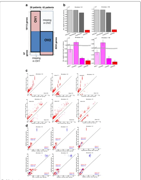
Fig. 4aIllustrationof the two OV datasets used for evaluating INSPIRE.Rowsrepresent genes andcolumnsrepresent samples.bFork= 91 (left) andk= 82 (right), INSPIRE is compared to WGCNA variants (top) and MGL variants (bottom) in terms of the best cross-validation (CV) negative test log-likelihood (lower is better) across all tested sparsity tuning parameters (λ).cFork= 91, INSPIRE (y-axis) is compared to each of the six competing methods (x-axes) in terms of the best−log10pfrom the functional enrichment of the learned modules. Eachdotis a KEGG, Reactome, or BioCarta GeneSet, and only the GeneSets with a Bonferroni correctedp<0.05 in at least one of the compared two methods are shown on eachplot. For MGL variants and INSPIRE, results from multiple runs are shown. We only considered the GeneSets with sufficiently different significance between the two methods, i.e. | log10p(INSPIRE)−log10p(ALTERNATIVE_METHOD)|≥δ.δ= 6 here and the results were consistent for varyingδ.dFork= 91, INSPIRE (y-axis) is compared to each of the six competing methods (x-axes) in terms of the best−log10pfrom the ChEA enrichment of the learned modules. Eachdot is for a gene set composed of a TF and its targets, and only the sets with a Bonferroni correctedp<0.05 in at least one of the compared two methods are shown on each plot. For MGL variants and INSPIRE, results from multiple runs are shown. We only considered the TFs with sufficiently different significance between the two methods, i.e. | log10p(INSPIRE)−log10p(ALTERNATIVE_METHOD)|≥δ.δ= 3 here and the results were consistent for varying

We used CRAN R package missMDA [56] to generate the imputed data.

Initialization of the INSPIRE latent variables

INSPIRE is an iterative learning algorithm that consists of three update steps, Eqs. (3)–(5), to learn the following sets of parameters: L, values on the latent variables, Z, gene-module assignments, and θL, the dependency net-work among the latent variables. So we need to have some starting point, i.e. initial values on any of these three sets of parameters. SLFA and MGL are also itera-tive learning algorithms that require a starting point. Therefore, for INSPIRE, SLFA, and MGL, we used the same initial gene-module assignments obtained by run-ning the k-means clustering algorithm on the imputed data (see above) because the imputed data contain all genes and all samples.

To be more specific, the authors of the MGL algo-rithm suggested initializing MGL withk-means centroids and we followed that approach for the MGL variants (MGL1, ImpMGL, and InterMGL) in our experiments. Given that INSPIRE is an extension to MGL for multi-data setting, to directly test whether the INSPIRE out-performs MGL, we used the output of MGL as a starting point for INSPIRE. The authors of the SLFA algorithm did not specify any initialization method; so for a fair

comparison among all these methods, we used the same initial gene-module assignments for SLFA and MGL—the centroids obtained by running the k-means clustering al-gorithm on the imputed data. The result of the k-means clustering algorithm also depends on the initial clusters which are randomly determined. So, to rule out the possi-bility to make a conclusion based on a particular set of ini-tial parameters, for every experiment on comparison across methods, we performed 10 runs with different ini-tial parameters (i.e. different random iniini-tial clusters in the k-means clustering algorithm) and presented the average results.

Runtime of INSPIRE on gene expression datasets

Running INSPIRE with the module count parameter k= 90 and the sparsity tuning parameter λ= 0.1 in our application on nine datasets (Additional file 1: Table S1) with a total number of p≅20,000 genes and n≅1500 samples took 13.7 min on a machine with an Intel(R) Xeon(R) E5645 2.40GHz CPU and 24GB RAM, once the latent variables are initialized. As mentioned above, for initialization of the latent variables, we used the module graphical lasso (MGL) [11] method on the imputed data, which took 10.2 min on the same machine.

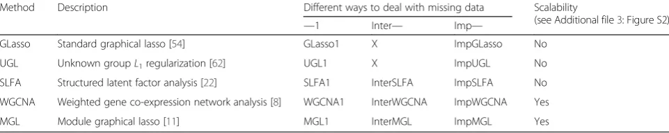
Table 1Methods we compared with the INSPIRE framework; To our knowledge, there are no published methods for learning modules and their dependencies that can handle variable discrepancy. We adapted the following five state-of-the-art methods that can run on a single dataset: GLasso - standard graphical lasso [54], UGL - unknown groupL1regularization [62], SLFA - the structured latent factor analysis [22], WGCNA - weighted gene co-expression network analysis [8], and MGL - module graphical lasso [11] (see

“Methods”for details). We adapted the input datasets such that we can apply these methods to datasets with variable discrepancy (Additional file 2: Figure S1B):“—1”, learning a model from only Dataset1 that contains all genes;“Inter—”, learning a model from the data on the overlapping genes (blue-shaded region in Fig. 1) and assigning the rest of the genes to learned modules by using thek-nearest neighbor approach (i.e. based on the Euclidean distance between the gene’s expression and the expression of each of the modules); and“Imp—”, imputing missing values in Dataset2 and learning a model from the imputed data (see“Methods”for details on imputation) (Additional file 2: Figure S1B). These adaptations lead to 13 competitors: (1) GLasso1; (2) ImpGLasso; (3) UGL1; (4) ImpUGL; (5) WGCNA1; (6) InterWGCNA; (7) ImpWGCNA; (8) SLFA1; (9) InterSLFA; (10) ImpSLFA; (11) MGL1; (12) InterMGL; and (13) ImpMGL. In the experiments on synthetic data, we compared to all 13 methods, while in the experiments with two genome-wide ovarian cancer gene expression datasets which we will discuss in the subsequent sections, we only used the methods that are scalable (see Additional file 3: Figure S2) These methods are indicated by the purple-shaded region in the table. The“Inter—” method is not applicable to GLasso and UGL, because GLasso and UGL learn a network of genes, not modules, and it is not obvious how to connect the genes that are present only in Dataset1 to the learned network. We do not consider an adaptation that applies the methods to Dataset2 only (“—2”). This is because, other than the genes in the overlap, Dataset2 has no genes (in the synthetic data experiments) or a very small number of genes (in the experiments with genome-wide expression data), which makes“—2”that uses only the samples from Dataset2 unlikely to outperform“Inter—”that uses all samples

Method Description Different ways to deal with missing data Scalability

(see Additional file3: Figure S2)

—1 Inter— Imp—

GLasso Standard graphical lasso [54] GLasso1 X ImpGLasso No

UGL Unknown groupL1regularization [62] UGL1 X ImpUGL No

SLFA Structured latent factor analysis [22] SLFA1 InterSLFA ImpSLFA No

WGCNA Weighted gene co-expression network analysis [8] WGCNA1 InterWGCNA ImpWGCNA Yes

Synthetic data generation

We synthetically generated data based on the joint distri-bution in Eq. (1). We first generated the sparsek×k in-verse covariance matrixλby creating ak×kmatrix G as

∀i;Gii¼0;

Gijði>jÞ_e

0 w:prb: ð1−dÞ

Uniform distribution 0ð ; 0:5Þ w:prb: d 2 ;

Uniform distribution 0ð :5;1Þ w:prb:

d

2 8

> > > > < > > > > :

and letting ΣL−1=G+GTso that ΣL−1 is symmetric. We set ∀i, Gii= afterwards by selecting such that the

resulting matrixΣL−1is positive definite.d ∈[0, 1] con-trols the density of ΣL−1 and the results we reported from synthetic data experiments were generated using k = 10 and d= 0.2. The results were consistent for varying values of kand d.

Then, we generated the latent variables L= {L1, …,Lk} from L~N(0, ΣL) and we randomly generated a binary pT×k matrixZ of module assignments which randomly assigns each ofpTgenes to exactly one of the latent vari-ables. Then we generated a high-dimensional data matrix XofpTgenes from the distributionX|ZL,σ

2

~N(ZL,σ2) and selected a portion of the samples and genes inX to form a smaller dataset that we call “Dataset1.” Then we selected the remaining samples and a portion of the genes fromXto form a second“Dataset2.”

We considered three simulated settings that correspond to different amount of overlapping genes (Additional file 2: Figure S1A). Each setting is characterized by [OL, D1, D2] where OL denotes the number of genes that are present in both Dataset1 and Dataset2, D1 is the number of genes that are present only in Dataset1 and D2 means the number of genes that are present only in Dataset2. The settings we consider are [150, 100, 0], [200, 50, 0] and [250, 0, 0], where the sample sizes of Dataset1 and Dataset2 are 20 and 30, respect-ively (Additional file 2: Figure S1A). [250, 0, 0] means that all genes are shared between the two datasets. We repeated the generation of data X 20 times in each of the three settings and presented the mean of the results for each method in (Fig. 3a–c). We show the p values on the bars that represent the statistical significance of the difference between each method and INSPIRE across 20 different data instantiations.

Additional file 2: Figure S1A illustrates the two data-sets in each of these three settings. In each rectangle, each row represents a variable and each column repre-sents a sample. For simplicity in presentation of the evaluation results, we set D2 = 0. The results were con-sistent for varying D2. We note that D2≅0 assumption

holds in many real-world settings we are interested in, where the newer technology contains almost all of the genes in the older technology. We demonstrate this real-world situation in the second set of experiments on the ovarian cancer expression data (Fig. 4b).

Comparison of the scalability across all six methods in simulation experiment

Computing the cross-validation test log-likelihood We performed a fivefold CV to choose λ for INSPIRE and each of the competing methods in our experiments to evaluate INSPIRE (synthetic data experiments and the experiments with two gene expression datasets). We measured the CV test log-likelihood on the test data portion of the first dataset (Dataset1 or OV1 which con-tains all or almost all genes) in each fold, which was common test data across all methods. For each of the five test folds, we computed the test data log-likelihood of the p×p gene-level dependency matrix that is com-puted using the dependencies among the latent variables (representing modules) inferred by each of the INSPIRE and its competitors, where p is the total number of genes in the two datasets. For the methods that optimize a non-convex objective function, we averaged the CV test log-likelihoods across multiple runs with different initial assignment of genes to modules. We tested a range of sparsity tuning parameter values (λ) and ob-served the “cup-shaped” underfitting/overfitting pattern in the λ (x-axis) versus average CV test log-likelihood (y-axis) curves for all methods, as expected.

Evaluation of learned network in synthetic data experiments

In the synthetic data experiments, the correspondence between the modules in a learned model and the mod-ules in the true model is not clear because each method can end up having different optimal number of modules, even if they started with the same number of initial modules. Therefore, we compared the methods in terms of the accuracy of the p×p gene-level dependency matrix that is computed using the dependencies among the modules inferred by each of the INSPIRE and its competitors, wherepis the total number of genes in the two datasets.

Measuring the significance of difference between INSPIRE and 13 competing methods

We repeated the synthetic data generation 20 times in each of the three settings, and presented the average results with the Wilcoxon signed rank testpvalue meas-uring the significance of differences based on the Wilcoxon signed rank test. More specifically, it measures the probability that the corresponding method gave a better result in terms of mean rank than INSPIRE across 20 different data instantiations.

Comparison of the prediction performance with alternative methods

We compared INSPIRE with PCA [18] and the subnet-work analysis method [13] based on how well each method can predict each of the six phenotypes (resectability as de-fined by 0 cm of residual tumor versus >0 cm of residual

tumor after surgery, survival time, and four manually cu-rated histologic phenotypes) from TCGA data. We used the lasso [58] (L1regularized linear regression) for predict-ing the continuous-valued phenotype (percent stroma), L1 regularized logistic regression for predicting binary pheno-types (stroma type, vessel formation, invasion pattern, and residual tumor), and L1 regularized Cox regression for predicting survival. The prediction performance was mea-sured in left-out data via leave-one-out cross-validation (LOOCV) tests for histologic phenotypes that have rela-tively less number of samples (~100) and 50-fold CV for resectability and survival that have larger number of sam-ples (~500). To evaluate a survival prediction model in a CV setting, we used two different methods to summarize the prediction results across CV tests. This is because un-like other phenotypes, the prediction performance on sur-vival time is measured by a ranking-based metric—the concordance index (CI) that measures the proportion of pairs of samples whose observed survival are concordant with the predicted survival in terms of which of the two samples experienced an event (death) before the other (or survived shorter) [59]. First, we predicted the survival (i.e. hazard scores) of all ~500 samples (specifically, 550 samples) when each sample was treated as a test sample in one of the 50 folds. Then we computed one CI value based on these predicted survival across all 550 samples, which leads to Fig. 5b (middle). Second, we considered computing CIs within test samples in each fold, which would allow us to have multiple CIs (# of folds × # of CV rounds) and compute the confidence interval of the CIs for INSPIRE compared to the CIs for the alternative methods (Fig. 5b, right). Especially, in this analysis, we performed 50 rounds of tenfold CV tests, and reported the average of a total of 500 CIs (i.e. y-axis of Fig. 5b, right) together with the associated Wilcoxon signed rank testpvalue measuring the significance of the difference between INSPIRE and each of the alternative methods (PCA-based method [18], subnetwork analysis [13], and individual genes). Allp values are smaller than 0.01 which means that the population mean of CIs from INSPIRE is statistically significantly higher than the popu-lation mean of CIs from each of the alternative methods. For each of the alternative methods, we also report the 95 % confidence interval for the mean of a normal distri-bution fitted to the difference of the method’s CIs from INSPIRE’s CIs. Given that all of the three intervals cover the positive-valued ranges, we can say that INSPIRE pre-dicts survival better than the alternative methods with 95 % confidence.

correlated with the phenotype, respectively. The subnet-work analysis method runs on binary phenotypes, but “percent stroma” is continuous-valued; so, to make the subnetwork method work on this phenotype, we binar-ized the values by making >50 % to be 1 and >50 % be 0.

Learning subtypes based on the INSPIRE latent variables We used the k-means clustering algorithm on the INSPIRE latent variables, each of which corresponds to a module, to cluster patients into four subtypes. We chose four as the number of subtypes to make it com-parable to alternative subtyping methods (TCGA study

[23] and the NBS method [60]). Since k-means is non-deterministic, the resulting subtypes could depend on the starting point of the subtype assignments. In order to get the most coherent groups of patients, we ran k-means ten times with different random initial as-signments of the patients into subtypes and chose the clustering which gives the lowest within cluster sum of squares.

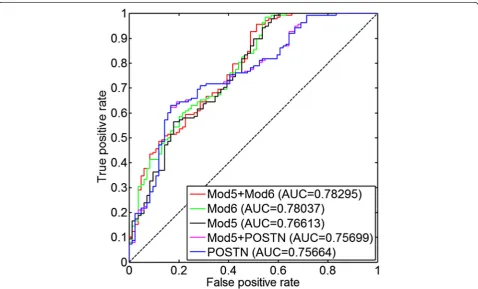
Supervised model to predict tumor resectability

We trained supervised models of tumor resectability using different combinations of the POSTN expression

b

a

d

c

Fig. 5aFor each of 90 INSPIRE modules (x-axis), the−log10pfrom the Pearson’s correlation is shown (y-axis) for six different histological and clinical phenotypes. Thepvalue threshold (shown byred dotted horizontal lines) is 5 × 10–3for histological phenotypes and 5 × 10–2for clinical phenotypes, which are harder to predict. We highlight modules 5, 6, 53, 54, 60, 78, and 81 that are significantly correlated with at least three of the six phenotypes inred. We also highlight module 30 inredsince it is the only module that has a significant correlation with the vessel formation phenotype. Modules 5 and 6 achieve the first or second rank in terms of the significance of correlation with five of the six phenotypes.

bFor four different methods (the subnetwork markers, PCs, all genes, and INSPIRE latent variables), the prediction performance is compared for six prediction tasks in CV setting. In allbar chartsexcept for the last one, a single accuracy (or concordance index for survival) is reported based on the predicted phenotype vector formed by pulling together the predictions for all folds. For the survival phenotype, an additional analysis is presented where the mean concordance index is reported across all 500 folds in 50 rounds of tenfold CV tests. For this bar chart (right), thep

and the latent variables corresponding to module 5 and module 6 in TCGA ovarian cancer data for 489 patients to predict 0 cm of residual tumor versus >0 cm of residual tumor. The proportion of the sub-optimally debulked pa-tients was 62 % (=139/223) in Tothill [34] and was 77 % (=378/489) in TCGA [23]. Logistic regression was used to train the models. Five distinct models were constructed: (1) a model with only thePOSTNexpression; (2) a model with only the latent variable corresponding to module 5; (3) a model with only the latent variable corresponding to module 6; (4) a model withPOSTNexpression and the la-tent variable corresponding to module 5; and (5) a model with the latent variables corresponding to module 5 and module 6. We trained each of those models along with (Fig. 6) and without (Additional file 4: Figure S3) the clin-ical covariates of age and stage. Performance was deter-mined based on the results of each fitted model in the Tothill [34] data in terms of the area under the curve (AUC) measure from a receiver operator characteristic (ROC) curve (Fig. 6 and Additional file 4: Figure S3).

Extraction of tumor histologic phenotypes from TCGA images

We manually curated multiple tumor histopathology fea-tures from image data on H&E staining of ovarian tumor

section from TCGA. We primarily used 98 randomly sampled patients to test the association between tumor histopathology features and the latent variables learned by INSPIRE. Features were curated in a blinded fashion. Five histopathological features were evaluated including percent stroma, percent tumor, vessel formation, stroma type, and pattern of invasion. Percent tumor was defined as the percent area involved by viable neoplastic cells across the entire slide while percent stroma was the per-cent area of fibrous tissue (fibroblasts and collagen). Vessel formation was scored as minimal, moderate, or abundant based on the number of formed vessels identi-fied at 100X magnification. Stroma type was defined as fibrous (dense collagen with relatively fewer fibroblasts) or desmoplastic (many fibroblasts embedded in a loose, myeloid extracellular matrix). Pattern of invasion related to how the neoplastic cells interacted with the surround-ing stroma and was scored as expansile, infiltrative, pap-illary, or mixed. Expansile invasion was characterized by cohesive tumor cells growing in a cluster with relatively well-circumscribed borders with the surrounding stroma while infiltrative invasion included tumor cells which grew in small nests or tentacles with abundant stroma surrounding the individual tumor cells. Tumors classi-fied as having papillary invasion had abundant

fibro-Fig. 6ROC curveof the supervised models for resectability prediction trained in TCGA and tested in Tothill data. Different combinations ofPOSTN

vascular cores upon which the neoplastic cells grew in arborizing branches. Mixed invasion patterns were iden-tified and classified as such.

Immunohistochemistry

Ten patients were sampled for staining based on either having good tumor resection and survival (>3-year survival, optimal debulking with residual tumor <1 cm) versus poor tumor resection and survival (<3-year survival, >1 cm residual tumor). Tissue and clinical in-formation were collected with patient consent by the University of Washington Gynecologic Oncology Tissue Bank under approval from the human subjects division (IRB 27077). Tumor tissue was collected at the time of primary surgery and flash frozen in liquid nitrogen, trans-ported to the lab and stored at –80 °C. The 17 frozen block was cryo-sectioned and one 8 mm section placed on a charged slide for IHC testing and H&E staining.

Frozen tissue slices fixed to glass slides were allowed to thaw at room temp for 10 min. Slides were fixed in a Coplin jar in cold acetone for 10 min at –20 °C. Slides were removed from acetone and placed tissue side up on a shaker. Phosphate buffered saline (PBS) was added to the slide (1 mL, enough to cover tissue slice) for 5 min shaking. PBS wash was repeated for a total of two 5 min washes. After the final wash, PBS was poured off the slide and tissues were blocked with 2 % milk/PBS (Carnation Instant Nonfat Dry Milk dissolved in PBS) for 1 h at room temperature, while shaking. Blocking so-lution was removed and primary antibody added, diluted in 1 % milk. Antibody dilutions were per manufacturer’s recommendations. Slides were allowed to incubate over-night at 4 °C while shaking with the primary antibody. If the primary antibody was conjugated to fluorescent mol-ecule, slides were also incubated in the dark overnight. Slides were washed three times with PBS at room temperature. The secondary antibody was diluted in 1 % milk/PBS and incubated at room temperature for 30 min, shaking. Slides were then washed with PBS for 10 min, three times. Nuclear stain diluted in PBS was added to tissues. Either Dapi (300 ng/mL, Sigma-Aldrich, catalog # D9542) or Sytox Green Nuclear Stain (Life Technologies, catalog # S7020) was used depending on the secondary antibodies used for staining. The last PBS wash was done at room temperature for 5 min. Coverslips were mounted to slides using Fluoroshield (Sigma-Aldrich, catalog # F6182) and sealed with clear nail polish. Images were taken on a Nikon TiE Inverted Widefield Fluorescence High Resolution Microscope.

Primary antibodies used were: Anti-E Cadherin anti-body conjugated to Allophycocyanin (Abcam, catalog no. ab99885); Hop Antibody (Santa Cruz, catalog no. sc-30216); Anti-CD73 antibody (Abcam, catalog no.

ab54217); and GCS-a-1 Antibody (Santa Cruz, catalog no. sc-23801)

Secondary antibodies used were: CD73 antibody was detected with Goat anti-mouse IgG-FITC (Santa Cruz, catalog no. sc-2010); when co-stained with CD73, HOPX was detected with Donkey anti-rabbit IgG-CFL 647 (Santa Cruz, catalog no. sc-362291); when co-stained with E Cadherin, HOPX antibody was detected with Chicken anti-rabbit IgG H&L FITC (Abcam, catalog no. ab6825).

Analysis of immunohistochemistry

Fluorescence images were analyzed using ImageJ [61] and the plugin JACoP was used for co-localization analysis.

Results

Overview of the INSPIRE framework

INSPIRE extracts a LDR from multiple gene expression datasets by inferringklatent (unobserved) variables and the dependencies among the latent variables captured by a probabilistic graphical model (Fig. 1). INSPIRE uses a standard iterative learning algorithm to optimize the joint log-likelihood objective function, Eq. (1), by itera-tively updating its model parameters until convergence (see“Methods” for details). INSPIRE iterates the follow-ing three steps until convergence: (1) inferrfollow-ing the values of latent variables with all the other parameters held fixed, as described in Eq. (3); (2) assigning genes into la-tent variables as described in Eq. (4); and (3) learning a network of latent variables as described in Eq. (5). In each iteration, latent variables are computed based on the current assignment of genes into modules and the estimated dependency network among the latent vari-ables, as described in Eq. (3). If there are no dependen-cies among latent variables, each latent variable would be an average expression level of the genes in the mod-ule. Thus, latent variables can be viewed as module cen-ters adjusted for the estimated dependency network among latent variables.

The number of moduleskis determined based on the standard Bayesian Information Criterion (BIC), although users can determine k in a different way depending on the problem. INSPIRE framework simultaneously infers the assignment of genes into k latent variables and the dependency network among k latent variables by fitting the probabilistic model across multiple gene expression datasets that can potentially have different sets of genes (e.g. different platforms) (see “Methods”). The INSPIRE model provides a biologically intuitive LDR model for gene expression data where many biological networks are modular and genes involved in similar functions are likely to be connected more densely with each other. How genes are organized into modules and how these modules are connected with each other would provide improved insights into the underlying disease process, as discussed below.

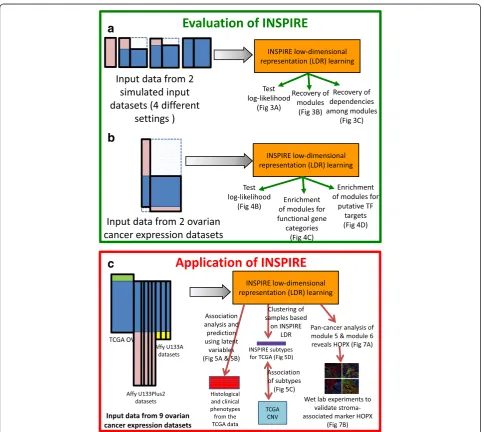
After evaluating INSPIRE by comparing with alterna-tive methods on simulated data and a small set of genome-wide expression datasets (Fig. 2a, b), we applied INSPIRE to many ovarian cancer expression datasets, which lead to a novel marker and potential driver of tumor-associated stroma (Fig. 2c).

INSPIRE learns underlying modules and their

dependencies from simulated data more accurately than 13 other methods

We first evaluate INSPIRE on data simulated using a probabilistic model of (unobserved) latent variables, gene expression levels, and the dependencies among the latent variables captured by a probabilistic graphical model (Fig. 1). To simulate the situation in which we are given expression datasets that contain different sets of genes (e.g. different microarray platforms), we generated two datasets (Dataset1 and Dataset2) with the same genes and included all genes in Dataset1 and varying percentages of the genes in Dataset2 such that varying numbers of genes are present in the overlapping portion of the datasets. This leads to three settings (Additional file 2: Figure S1A, Fig. 3a (ii)–(iv) left): (ii) 60 % of the genes are present in Dataset2, (iii) 80 % of the genes are present in Dataset2; and (iv) all genes are present in Dataset2. The total number of genes in each of these set-tings is 250, and the number of modules is 10, with an average of 25 genes in a module (see “Methods” for de-tails of synthetic data generation).

We compare INSPIRE with the following five state-of-the-art methods: (1) GLasso, standard graphical lasso [54] that learns a gene-level conditional dependence net-work with no LDR or module assumption; (2) UGL, un-known group L1 regularization [62] that learn sparse block-structured inverse covariance matrices with un-known block structure; (3) SLFA, structured latent factor analysis [22] that learn an LDR of the data as well as the

relationship between the latent factors; (4) WGCNA, weighted gene co-expression network analysis [8] that allows to define modules based on a special metric derived from the correlations of the gene pairs; and (5) MGL, module graphical lasso [11] which simultaneously learns a LDR and the conditional dependencies among the latent variables (Table 1). Since all those methods work on a single dataset, to enable the application of these methods to multiple datasets with variable discrep-ancy, we adapt the input data to those five methods in three ways (Additional file 2: Figure S1B): (1) using only Dataset1 that contains all genes; (2) using data on the genes that are present in both datasets (blue-shaded re-gion in Fig. 1), and assigning the rest of the genes to the learned modules based on the Euclidean distance be-tween the gene’s expression and the expression of each of the modules; and (3) imputing missing values in Dataset2 and using both datasets as if they were a single dataset. This leads to 13 methods (Table 1). InterMGL, ImpMGL, and INSPIRE represent different ways of handling missing data: INSPIRE uses a novel learning al-gorithm that does not require the missing portion when learning; ImpMGL imputes missing variables in the datasets before learning; and InterMGL ignores missing variables in the datasets. We run each method on 20 dif-ferent instantiations of the synthetic data and present the average results with p values of significance of the difference with INSPIRE (see “Methods”; Fig. 3). We evaluated INSPIRE and 13 competitors in terms of how well they explain unseen data measured by the test-set log-likelihood, gene-module assignment accuracy, and the module dependency network accuracy. In order to make comparisons with WGCNA variant methods pos-sible, we applied a standard graphical lasso algorithm to the modules learned by a WGCNA variant method. INSPIRE, SLFA, and MGL are iterative algorithms with non-convex objective functions, so their results may de-pend on the initialization of the parameters. To rule out the possibility of making a conclusion based on a par-ticular set of initial parameters, we performed the variants of those algorithms multiple times with dif-ferent starting points (see “Methods” for details on initialization).

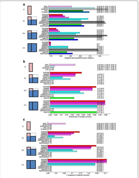
Test log-likelihood

measured on Dataset1 in X (see “Methods”). We used the test set of Dataset1 to compute the test log-likelihoods for all methods since Dataset1 contains all genes. Figure 3a shows the average negative test log-likelihood per sample (lower the better) in (i)–(iv): (i) shows the methods that use only Dataset1 and (ii)–iv) show Imp—, Inter— and INSPIRE methods that use Dataset2 as well with varying numbers of genes in Dataset2 (Additional file 2: Figure S1A). Each bar (except INSPIRE) displays a p value from the Wilcoxon signed rank test that measures how significantly INSPIRE is better than the corresponding method across 20 instantiations of the data (see “Methods”). The bars for the methods that use only Dataset1 display three p values, each for comparison to INSPIRE in (ii)–(iv). INSPIRE has significantly better test log-likelihoods than the methods that utilize one dataset (p≤2.4 × 10–5) and all the other eight methods that can utilize mul-tiple datasets (p ≤4.3 × 10–4). This indicates that mak-ing use of multiple datasets by usmak-ing INSPIRE has great potential to increase the chance to infer the true underlying model. In (iv), ImpMGL, InterMGL, and INSPIRE perform similarly as expected, and they are better than the other methods that utilize mul-tiple datasets. The methods that utilize only Dataset1 (i) achieve worse average test log-likelihood than their multiple-dataset counterparts (ii)–(iv); and the test log-likelihood of most methods increase with the increasing number of overlapping variables, from (i) to (iv).

Module recovery

We then evaluated how well important aspects of the true underlying model are recovered by each method. We first checked whether pairs of genes that are assigned to the same module in the true model are in the same modules in the learned model. We used the rand index [65] that measures how well pairs of genes agree on being in the same or different modules between two models—the true model and a learned model. A rand index of 0 means that none of the genes agree on being in the same/different groups, while 1 means a per-fect recovery of the modules. The evaluation based on module recovery is not applicable for GLasso1 and ImpGLasso, since they do not learn modules. As shown in Fig. 3b, the module recovery performance of INSPIRE is significantly better than its 13 competitors. INSPIRE has a significantly higher rand index than (i), the methods that utilize a single dataset (p ≤4.9 × 10− 2), and (ii)–(iv), the methods that use multiple datasets (p≤6.6 × 10−2).

Module dependencies

Then, we evaluated how well the inferred module de-pendencies by each method are consistent with those in

the true model. Since it is not clear how to map a module in the true model to the corresponding module in the learned model, we converted each module-based network model into the equivalent gene-based probabilistic model using a well-established method [11]. It is not enough to get only high precision or recall, so we used the F−measure

¼2_ðð_precprec_þrec_recÞ_Þ as an evaluation metric. As shown in Fig. 3c, INSPIRE has the highest average F-measure that measures the accuracy of the dependencies learned by each method in (i)–(iv). INSPIRE is signifi-cantly better than methods that utilize a single data-set (p ≤2.4 × 10–4) and other methods that use multiple datasets (p≤2.7 × 10–2).

The methods that use only one dataset tend to have a lower average rand index (for modules) and F-measure (for module dependencies) than their multiple-dataset counterparts; and as the number of genes shared across datasets increases, the overall performance of the methods that utilize multiple datasets increases. This in-dicates that combining multiple datasets reveals under-lying modules and their dependencies better; INSPIRE is better than 13 alternative approaches in revealing the underlying model.

Evaluation on two genome-wide ovarian cancer expression datasets

Next, we evaluated INSPIRE based on the statistical ro-bustness and biological relevance of the learned modules on two publicly available ovarian cancer gene expression datasets [31] (Fig. 4a): (1) OV1 that contains 18,113 genes and 28 patients (Affy U133 Plus 2.0 platform); and (2) OV2 that contains 8331 genes in a total of 42 patients (Affy U95Av2 platform) (see“Methods”; Additional file 6: Table S2).

In the next three subsections, we show the results of the following evaluations (Fig. 2b): (1) how well the INSPIRE model fits unseen data measured by test log-likelihood; (2) the statistical significance of the overlap between the learned modules (i.e. gene-module assign-ment) and known functional gene sets; and (3) how well the learned modules reflect putative regulatory relation-ships between TFs and targets based on the ChEA database [66].

INSPIRE learns a statistically more robust LDR model than alternative approaches

We first evaluated the learned LDR model based on the test-set log-likelihoods that measure how well the learned model can explain left-out test data in OV1 through the standard fivefold CV tests (see “Methods”). We used the test set of OV1 for computing the test log-likelihoods for all compared methods since OV1 con-tains almost all of the genes contained by either of the datasets. In Fig. 4b, the best average test log-likelihood per sample across the tested λ values is plotted for each method. As can be seen in Fig. 4b, INSPIRE achieves better test log-likelihood than six alternative methods, WGCNA1, InterWGCNA, ImpWGCNA, MGL1, InterMGL, and ImpMGL (Table 1) for bothk= 91 chosen by the BIC score (left panel) and k= 182, an alterna-tive k value that results in modules with average size of 100 (right panel). Since MGL and INSPIRE may depend on the initialization of the model, the stand-ard deviation across ten runs of those methods with different initializations are represented by the error bars on the bottom panel in Fig. 4b.

INSPIRE modules are more significantly enriched for functional gene sets than alternative methods

INSPIRE uses a biologically intuitive LDR model for expression data, in which genes are assigned to k modules, and each module can be interpreted as bio-logical processes performed by the genes in that mod-ule. Thus, whether each module is enriched for the genes that are known to be in the same functional categories can be a way to evaluate the biological relevance of the LDR inferred by INSPIRE. Here, we evaluated INSPIRE based on whether the learned modules are significantly enriched for known path-ways from MSigDB [67]. We compared INSPIRE with six alternative methods, WGCNA1, InterWGCNA, ImpWGCNA, MGL1, InterMGL, and ImpMGL (Table 1), usingk= 91 chosen by the BIC score andk= 182, an alter-nativekvalue that results in modules with average size of 100. For each method, we choseλ that achieves the best CV test log-likelihood, a standard technique [64].

We considered 1077 GeneSets (pathways) from the C2 collection (curated gene sets from online pathway

databases) of the current version of the MSigDB [67] based on Reactome [68], BioCarta, and KEGG [69]. We excluded the pathways based on computational predic-tions from this collection. We computed the significance of the overlap between each GeneSet and each module measured by the Fisher’s exact test pvalue, followed by the Bonferroni multiple hypothesis correction. Figure 4c and Additional file 7: Figure S5A show the results of the functional enrichment analysis for k= 91 (chosen based on BIC) and k= 182, respectively. In each scatter plot, a larger portion of the dots lie above the diagonal, which implies that the INSPIRE modules are more significantly enriched for known pathways than those inferred by the alternative approaches. This indicates that INSPIRE is better at identifying biologically coherent modules based on prior knowledge more accurately than the alternative methods.

INSPIRE modules are more significantly enriched for putative targets of the same TF than alternative approaches

As an alternative way to evaluate the biological coher-ence of the learned modules, we checked how signifi-cantly the modules are enriched for the genes that have been shown to be bound by the same TFs. The ChEA database [66] provides a large collection of TF-target in-teractions captured in previously published ChIP-chip, ChIP-seq, ChIP-PET, and DamID (referred herein as ChIP-X) data. For each of 107 TFs in the ChEA database [66], we computed the significance of the overlap be-tween each module and each TF’s putative targets from ChEA database measured by the Fisher’s exact testpvalue followed by the Bonferroni correction. Figure 4d and Add-itional file 7: Figure S5B show the results of our ChEA en-richment analysis fork= 91 (chosen based on BIC) andk = 182, respectively. In each scatter plot, a much larger por-tion of the dots lie above the diagonal, which indicates that INSIRE modules are biologically more coherent, i.e. more significantly enriched for putative targets of the same TF. In Fig. 4d and Additional file 7: Figure S5B, we indicate with a blue dot a TF that resides in the same module as the module that is enriched for the TF’s puta-tive targets. We do not expect all dots to be blue (i.e. all TFs being in the same modules as their putative targets), because the protein level of TF may not be correlated with its messenger RNA (mRNA) expression level. It is still in-teresting to see that INSPIRE modules are more signifi-cantly enriched for the genes that have been shown to be bound by the same TFs in ChIP-X data.

Application to nine genome-wide ovarian cancer expression datasets

comprising 1498 ovarian cancer patient samples downloaded from the TCGA project website and the Gene Expression Omnibus (GEO) [26] (Fig. 2c). This corpus of data consists of publically available tran-scriptomic characterizations of ovarian cancer across nine distinct studies where gene expression data col-lected in different studies come from distinct plat-forms. These data are therefore a perfect corpus to apply the INSPIRE method for a variety of reasons. First, there is a sufficient sample size across studies to resolve distinct modules that are robust across data-sets. Second, our method will outperform more naïve ap-proaches by imputing missing genes through leveraging shared structure across the data and will therefore increase the resolution to detect robust modules. Finally, there are known subtypes in ovarian cancer as identified by the TCGA ovarian cancer study [23] and we anticipate that our approach will not only re-identify these subtypes based on the ex-pression of our inferred modules, but will also further resolve potential molecular drivers of these subtypes through ancillary analyses of the INSPIRE inferred modules. These ancillary analyses are described below. We repeated our analyses for this application using varying module counts that correspond to the average number of 200, 140, and 100 genes, respectively, in each module and for varying sparsity tuning parameters

λ= {0.01, 0.03, 0.1}; and we observed that all results were highly robust for the varying values of k and λ. We re-ported results from our biological analysis for k= 90, as selected by BIC for thek-means clustering applied to the imputed data matrix, andλ= 0.1 which leads to the spars-est network of modules, given that sparsity is of key im-portance in learning and the interpretation of a high-dimensional conditional dependence network.

We evaluated the learned LDR consisting of 90 mod-ules and the corresponding latent variables based using three evaluation metrics:

(1)We performed gene set enrichment analysis to characterize each module based on its associated genes (see Additional file 8: Table S3 for the gene set enrichment analysis results together with the significance).

(2)We analyzed the associations between the learned latent variables, each representing a module, and six important phenotypes in cancer, including resectability, which was defined by the residual tumor size after surgery, survival, and four histopathological phenotypes manually curated based on the histopathology in the TCGA ovarian cancer data (see Additional file 8: Table S3), and we used inferred INSPIRE latent variables as features for predicting those phenotypes. Figure5a

shows the association between the learned latent variables with the six important phenotypes and Fig.5bcompares INSPIRE to the following based on the prediction of those phenotypes: (1) PCA [18], an unsupervised LDR method; (2) subnetwork analysis [13], a supervised LDR method; and (3) all genes when no LDR is learned. The histopathological phenotypes are provided as a resource for this paper (Additional file9: Table S4) and residual tumor size and survival are available on the TCGA web site. (3)We used the inferred latent variables to identify new

subtype definitions in ovarian cancer. We compared INSPIRE subtypes to: (1) the subtypes recently described by the TCGA ovarian cancer study [23]; and (2) the subtypes learned by a method that uses mutation profiles for the network-based stratification of cancer patients (NBS) [60], based on how relevant they are to genomic abnormalities in ovarian cancer. Detailed information concerning expression datasets used in the INSPIRE analysis is presented in Additional file1: Table S1 and the processing of the expression data is described in“Methods”.

(4)We perform both statistical and biological experiments to show thatHOPX is a potential molecular driver from tumor-associated stroma in a module that differentiates the patients with increased percent stroma, infiltrative stroma, and desmoplastic stroma.

Negatively correlated modules show distinct pathways and potential regulatory TFs enrichment

Additional file 10: Figure S6A (top) demonstrates that the modules that are strongly negatively corre-lated with each other show very distinct pathway (left) enrichment as well as TF binding enrichment (right). In Additional file 11: Table S5, the significance of enrichment from five negatively correlated module pairs with the biggest absolute correlation listed for five pathways or TFs for which the highest enrich-ment difference between the negatively correlated modules is observed.

We also compared between following two models in terms of functional enrichment of the modules: (1) two negatively correlated modules are defined as two separ-ate modules as in the original work; and (2) instead of the two negatively correlated module, there is one hypo-thetical module that contains all genes in the two nega-tively correlated modules. Additional file 10: Figure S6A (bottom) compares between model I (y-axis) and model II (x-axis) in terms of functional coherence based on the pathway database (left) and putative TF binding targets (right). Model I reveals more functionally coherent modules than model II, which justifies our modeling as-sumption that negatively correlated genes need to be in separate modules.

INSPIRE latent variables are significantly associated with clinical and histologic phenotypes in cancer

To gain relevant biological insight from ovarian cancer (OV) transcriptome data, we used the 90 inferred latent variables from the INSPIRE model as a LDR of tran-scriptomic profiles across patients (Fig. 2c) that captures robust cross-dataset patterns of gene expression. We evaluated the clinical relevance of these latent variables by measuring the statistical association between these la-tent variables and histopathological phenotypes of tumor. The morphological interpretation of histologic sections of tumor forms the basis of diagnosis, aggres-siveness assessment, and prognosis prediction. Patholo-gists examine the tumor diagnostic images based on semi-quantitative histologic phenotypes of the tumor such as invasion pattern and percent stroma to predict the aggressiveness of cancer. Identifying the molecular basis for these histologic phenotypes will advance the understanding of the molecular biology of ovarian can-cer. We manually examined five histologic phenotypes for 98 randomly selected patient images from TCGA: percent stroma, percent tumor, vessel formation, stroma type, and invasion pattern (details in “Methods”; Additional file 9: Table S4). For each pair of a histologic phenotype and a latent variable from the INSPIRE model, we performed the Pearson’s correlation test that produces a correlation coefficient and a p value. Additional file 8: Table S3 lists the pvalues from these association tests of INSPIRE latent variables, with each

of the five histologic phenotypes. Figure 5a shows the correlation of each latent variable with each of the histologic phenotypes. Since percent stroma and per-cent tumor phenotypes are almost perfectly (anti-) correlated, we only included percent stroma in Fig. 5a. We usedpvalues from a likelihood ratio test for a Cox proportional hazards model to determine the signifi-cance of association of a gene with patient survival and we usedpvalues from the Pearson’s correlation test for tumor resectability.

Modules 5 and 6 show high correlations with the histopathological phenotypes, such as percent stroma, stroma type, and invasion pattern. As shown in Fig. 5a, those modules are also associated with patient survival and tumor resectability. We observed that the quantity of residual tumor after surgery is posi-tively correlated with the amount of tumor-associated stroma, where increased residual tumor, i.e. low re-sectability, is an important and a previously known indicator of poor patient prognosis. Although the latent variables of modules 5 and 6 show high expres-sion correlation (the correlation coefficient between the module 5 latent variable and the module 6 latent variable is 0.84), these two modules are functionally fairly different. Additional file 10: Figure S6B com-pares modules 5 and 6 in terms of the pathways and putative TF targets that are enriched in these mod-ules. There are handful of dots that are distant from the diagonal line implying that modules 5 and 6 exhibit several unique biological properties. In Additional file 12: Table S6, the significance of enrichment from modules 5 and 6 are listed for five pathways or TFs for which the highest enrichment difference between the modules is observed.