Numerical test concerning bone mass apposition under electrical and mechanical stimulus

R E S E A R C H

Open Access

Numerical test concerning bone mass apposition

under electrical and mechanical stimulus

Diego A Garzón-Alvarado

, Angélica M Ramírez-Martínez

and Carmen Alicia Cardozo de Martínez

* Correspondence:dagarzona@unal. edu.co

1_{Research Group on Numerical}

Methods for Engineering (GNUM), Universidad Nacional de Colombia, Bogota, Colombia

3_{Biomimetics Laboratory.}

Biotechnonology Institute, Universidad Nacional de Colombia, Bogota, Colombia

Full list of author information is available at the end of the article

Abstract

This article proposes a model of bone remodeling that encompasses mechanical and electrical stimuli. The remodeling formulation proposed by Weinans and collaborators was used as the basis of this research, with a literature review allowing a constitutive model evaluating the permittivity of bone tissue to be developed. This allowed the mass distribution that depends on mechanical and electrical stimuli to be obtained. The remaining constants were established through numerical experimentation. The results demonstrate that mass distribution is altered under electrical stimulation, generally resulting in a greater deposition of mass. In addition, the frequency of application of an electric field can affect the distribution of mass; at a lower frequency there is more mass in the domain. These numerical experiments open up discussion concerning the importance of the electric field in the remodeling process and propose the quantification of their effects.

Background

Bones provide mechanical stability to the human body and are a source of minerals for metabolism [1]. Bones have been studied extensively from the mechanical and mineral standpoint, and in terms of functionality [1,2]. From a mechanical point of view, bones can be adapted to loads on trajectories of stress through mineral apposition, which is due to the action of osteoblasts [1-4]. Furthermore, they reabsorb minerals when the mechanical stimulus is sufficiently low, as it is unnecessary to maintain structure [2]. Reabsorption is directed by osteoclasts. Osteoblasts and osteoclasts are the primary cells involved during bone remodeling that are stimulated by the action of mechanical strain sensors, for example, osteocytes [2]. These three cell types play an important role during the processes of replacement, maintenance and modeling of bones [1].

Following the work of Meyer during the nineteenth century, Wolff [5] proposed a the-ory of trabecular bone architecture, which assumes that trajectories of high mechanical stress form the trabecular bone. In 1987, Frost [6-8] suggested an adaptive mechanism of bone mass as a function of mechanical stress. Consequently, several bone remodeling algorithms have been developed including those proposed by Frost [8], Pauwels [9], Kum-mer [10], Cowin [11-13] and Hegedus [14], which predict the formation of bone structure from internal mechanical loads studied in terms of stress and strain.

From mechanical models of bone remodeling, sophisticated studies have been car-ried out concerning the processes of apposition and reabsorption during bone

turnover, and particularly concerning the distribution of mass in the femur [15,16], hip replacement [17,18], and dental implants [19]. Generally, these studies have been phe-nomenological. Therefore, researchers have made significant efforts to include mathem-atical models and the role of cell biology and biochemistry in the remodeling process, resulting in research that begins at the microscopic level, concerning the effects of basic cellular remodeling units (BMU, Basic multicellular units) during tissue replace-ment [20,21]. From the perspective of BMU, important work was initiated at the bio-chemical and mechanical level concerning the effects of cracks [22], cell cycles throughout adult life [23], active molecules within each cell [24] and the spatial distri-bution of each BMU [25]. With these important advances in the understanding of bone remodeling, researchers in the field increasingly turned to the study of other biophys-ical stimuli that can affect this process. Most models have not taken account of the physical-chemical phenomena of tissue mechano-transduction. For this reason, new investigations that allow the piezoelectric and electrokinetic behavior of the bone to be studied were undertaken [26].

A clinical study demonstrated that a local electromagnetic field accelerates the heal-ing process after bone fracture [26]. Therefore, an article by Demiray and Dost [27] began new research concerning the effect of the electromagnetic field on interior injury to bone. In another article, Ramtani [26] presented a mathematical model relating to the benefit of the electric field in the reparair and maintenance of the solid matrix of bone. Furthermore, there are studies concerning the electrical behavior of bone tissue during the production of electric fields, and external electrical flow. Fukada and Yasuda [28] demonstrated that bone exhibits piezoelectric behavior, i.e. mechanical stress cre-ates electric polarization (the indirect effect) and an external electric field causes strain (the converter effect). In addition, the properties of bones that produce piezoelectric potentials have been determined [29-33]. These data led to the development of math-ematical models that include the effect of electromagnetic fields during the repair [34,35] and remodeling [36] of bone. For example, Qu and Yu [34] developed a math-ematical model (no spatial dimension) of the remodeling process and healing under the effect of mechanical loads and the use of electric charges. In this model, the higher the voltage applied to a bone after fracture, the lower the percentage of bone damage and micro damage in the few days after the stimulus. Similarly, during osteoporosis an elec-tric field increases bone density over time. Huang et al. [37] established a hypothesis concerning the biological and biochemical pathways that activate cells, particularly osteocytes, during the imposition of an electric field. Furthermore, Qu and Yu [38] pro-posed a mathematical model that included mechanical loads and electromagnetic effects during the process of bone remodeling.

apposition. Therefore, the model proposed herein can be used as a basis for further work concerning electrical effects in the maintenance of bone.

Methods

The electro-mechanical model

The electro-mechanical model of bone remodeling that involves mechanical and elec-trical stimuli can be written, hypothetically, as follows (1):

dρ

dt ¼gmechðρ;Wmecð Þρ Þ þgelectðρ;WelectðEðρ;fÞÞÞ ð1Þ

Wheregmechðρ;Wmecð Þρ Þis the well known mechanical stimulus described by Weinans [39], which depends on tissue density (ρðx;y;z;tÞ), and the work carried out by mech-anical stress (Wmecð Þρ ) andgelectðρ;WelectðEðρ;fÞÞÞis the electrical stimulus that depends on density, frequency and the work carried out by the electric field (WelectðEð Þρ Þ). Dur-ing this first approach, we consider that the two stimuli are added to determine the bone remodeling process. However, we will develop each of the terms that determine the electro-mechanical model throughout this article.

The mechanical model

Following the remodeling mechanical model described in [4,39], the density variation over time depends on the mechanical stimulus that exists at every spatial point of the bone, which can be written as in [39] (2):

gmechðρ;Wmecð Þρ Þ ¼k1

Wð Þρ Wrefm

1

ð2Þ

Where ρis the bone density at each point in space (ρðx;y;z;tÞ), Wð Þρ is the energy-strain per unit of volume due to mechanical stress, k1 is a constant and Wref m is the strain-energy (per unit of volume) of reference that sets the threshold for which they will perform deposition (Wð Þρ =Wrefm >1) or absorption (Wð Þρ =Wrefm <1) of the tissue

[39], in the presence of mechanical stress. It should be noted that the energy-strain depends on the density and is given by (3):

Wð Þ ¼ρ 1

2ρe

T_{Cð Þρ e ð3Þ}

Whereeis the strain, in Voigt notation, of the strain tensor given in (4):

e¼½E11 E22 γ12

T _ð

4Þ

That is a function of the displacements given by (5):

u¼½u1 u2T ð5Þ

e¼B1u¼

@

@x 0

0 @

@y

@ @y

@ @x 2 6 6 6 6 6 4

3 7 7 7 7 7 5

u1

In addition, Cð Þρ is the matrix of linear elasticity. The matrixCð Þρ contains the Pois-son module, which is usually considered constant, and Young's modulus that depends on the density by expression [4] (7):

Eð Þ ¼ρ Aρn ð7Þ

where A is a constant and n establishes a relationship of power density that has been uncovered through experimentation [39].

By manipulating equation (7) we can obtain a dimensionless form of the density. This is easier to use with the aim of determining the modulus of elasticity. Multiplying the right side of (7) by ρn

0=ρn0

produces (8):

Eð Þ ¼ρ Aρn

0

ρ ρ0

n

¼E0 _ρρ 0

n

¼E0λn ð8Þ

WhereE0¼Aρn0 andλ¼ρ=ρ0are the elasticity modulus and the dimensionless density

ratio, respectively. Therefore, the linear elasticity matrix can be expressed as (9):

Cð Þ ¼ρ λn_C

0 ð9Þ

Where C0 is the matrix of linear elasticity with constant coefficients, which depends

onE0andνonly, and is given in the case of plane stress by:

C0¼

E0

1ν2

1 ν 0

ν 1 0

0 0 1

2ð1νÞ

2 6 4

3 7

5 ð10Þ

Thus, the strain energy per unit of volume (3) can be expressed as (11):

Wð Þ ¼ρ 1

2ρλneTC0e¼λ

n

ρ

eT_C

0e

2

¼λ_ρnUmec ð11Þ

Where Umec is the strain energy at each instant of time, which is calculated with the initial constant of the remodeling [39] problem only. Replacing these equations in (2), and with some algebraic manipulation, we produce (12):

gmechðρ;Wmecð Þρ Þ ¼k1 ρ_ρ0 0

λn_U mec ρWrefm

1

¼k1 ρ_ρ0 λ

n_U mec ρ0Wrefm

1

¼k1 λn1

Umec ρ0Wrefm

1

ð12Þ

where we can defineUrefm ¼ρ0Wrefm. Therefore, we produce the following equation for

the density ratio (13):

gmech¼k1 λn1

Umec

Urefm

1

ð13Þ

The momentum equation that establishes the internal stresses of a body is given by [40] (14):

r σþb¼0 ð14Þ

Where the stress is given by (15):

σ¼C ρÞe¼λn_C

0e

Electrical model

This article proposes the inclusion of a hypothetical electrical term that can determine, in part, the process of bone remodeling. Therefore, the contribution of this stimulus can be written as (16):

gelectðρ;WelectðEðρ;fÞÞÞ ¼k2

WelectðEðρ;fÞÞ

Wrefe

ð16Þ

Where 2ðρ;fÞis the electrical permittivity of bone tissue and depends on the dens-ity, (ρ) where frequency (f), Welectð2ðρ;fÞÞis the electrical energy per unit of volume,

k2 is a constant andWref eis the electric energy (per unit volume) of reference.

It should be noted that the term electric energy depends on permittivity, which in turn depends on the density and frequency. This energy term is given by (17):

Welectð2ðρ;fÞÞ ¼ 1

2ρ2ðρ;fÞEðx;y;z;tÞ

2 _ð

17Þ

Where Eðx;y;z;tÞ is the electric intensity (electric field). However, Eðρ;fÞ, electrical permittivity, depends on density and frequency, and is given by (18):

2ðρ;fÞ ¼ 202rðρ;fÞ ð18Þ

Where 20is the permittivity in the free space and2rðρ;fÞis the relative permittivity, which in turn is given by (19):

2rðρ;fÞ ¼Bρmþδð Þf ð19Þ

where B is a constant and m establishes a relationship of power density that can be proved through experimentation, and will be developed in the following sections. Fur-thermore,δð Þf is a function of frequency at which the electric field is applied.

As with the mechanical case, we can manipulate equation (19) so that it is expressed in terms of relative density, multiplying the first term by to produce

ρn

0=ρn0

(20):

2rðρ;fÞ ¼Bρm0λ

m_þδ

f

ð Þ ¼ 2ρλm_þδ

f

ð Þ ð20Þ

where 2ρ is a constant for the power model of relative permittivity. Therefore, sub-stituting (20) in (17), we obtain (21):

Welectð2ðρ;fÞÞ ¼ 1 2ρ

ρ0

ρ0

20 2ρλmþδð Þf

Eðx;y;z;tÞ2 ¼_2ρ1

0λ

20 2ρλmþδð Þf

Eðx;y;z;tÞ2¼ 1

ρ0λ

2ρλm_{þδð Þf}

Uelect

ð21Þ

where Uelect¼1220Eðx;y;z;tÞ2. Substituting equation (21) in (16) produces (22):

gelectðρ;Welectð2ð Þρ ÞÞ ¼k2 1

ρ0λ 2ρλmþδð Þf

Uelect

Wrefe

¼k2 2ρλ

m_{þδð Þf}

λ

Uelect

Urefe

ð22Þ

We have chosenUrefe ¼ρ0Wrefe as the reference value of electric energy.

However, Gauss's law for an electric field, with no internal loads, is given by (23):

r D¼ρe ð23Þ

can be expressed in terms of a quantity called electric potential or voltage, given by (24):

E¼ rφ ð24Þ

whereφis the electric potential.In summary, equation (1) can be written as (25):

dρ

dt ¼k1 λ

n1Umec

Urefm

1

þk2

2ρλm_{þδð Þf}

λ

Uelect

Urefe

ð25Þ

Again, using the dimensionless form, we have (26):

dλ dt ¼

k1

ρ0

λn1Umec

Urefm

1

þk2

ρ0

2ρλm_þδ

f ð Þ λ Uelect

Urefe

ð26Þ

dλ

dt ¼kmec λ

n1Umec

Urefm

1

þkelect

2ρλm_{þδð Þf}

λ

Uelect

Urefe

wherekmec¼k1=ρ0andkelect ¼k2=ρ0 are mechanical and electrical constants that define

the conversion rate of bone remodeling, dependent on the mechanical stress and the electrical potential, respectively.

Solution by the finite element method

To solve equation (14) we take its differential form to its weak [40] form, to obtain (27):

Z

Ω δeλn_C

0edΩ

Z

Ω

δubdΩ

Z

Γ

δutdΓ ¼0 ð27Þ

Where δe and δu are weighting functions, and t¼σn is the traction on the boundaryΓ that serves as a frontier to the domainΩ(see Figure 1).

To calculate the approximate solution by finite element discretization, the displace-ment field approximates through [40] (28):

uðx;tÞ ¼NTðxÞa tð Þ ð28Þ

Where NTðxÞis a row vector containing the shape functions used to approximate the displacement að Þt [40] in the nodes. Using the Galerkin method, we approximate the weighting functions in the same way as the displacement field, producing at the elem-entary level equation [40] (29):

Z

ΩeBλ n_C

0BTdΩe

aþ Z

Ωe

NbdΩeþB:C:¼0 ð29Þ

whereBis the derivative operator (discrete version of operatorB1of equation (6)) that

converts the displacements into strains (see [40]). This system of equations is com-pleted by applying the Neumann and Dirichlet conditions suitable for solving the elastic problem (see Figure 1).

potential to produce (30):

Z

Ω

rw

ð Þ 2ρλm_þδ

f ð Þ

rφ

ð ÞdΩþ

Z

Ω

wρ_edΩ

Z

Γ

w2ρλmþδð Þf ðrφÞ ndΓ

¼0 ð30Þ

where w is the weighting function and n is the external normal to the domain of the problem. Again, for calculation of the approximate solution, the scalar field of the electric potential approaches through [40] (31):

φðx;tÞ ¼NTðxÞv tð Þ ð31Þ

Where v is the potential at each node of the element, and N xÞð are the shape func-tions for scalar [40] problems. Weighting funcfunc-tions are chosen in the same manner as shape functions, which is through the method of (Bubnov-) Galerkin standard. There-fore, at the elementary level we have the following equation (32):

Z

ΩBe 2ρλ m_þδ

f ð Þ

BT edΩe

vþ Z

Ω

NT_ρ

edΩþB:C:¼0 ð32Þ

where

Be¼ @N1

@x

@N1

@y

@N2

@x

@N2

@y

@Nnod @x

@Nnod @y 2 6 6 6 6 6 6 4 3 7 7 7 7 7 7 5

ð33Þ

wherenodis the number of nodes of each element.

Solution to the equation of relative density

This article solves the equation of dimensionless density (or relative) by integrating equation (26) by the method of Euler. For this purpose we define (34):

dλ

dt ¼fðx;tk;λ;fÞ ¼kmec λ

n1Umec

Urefm

1

þkelect 2ρλ

m_{þδð Þf}

λ

Uelect

Urefe

ð34Þ

Therefore, the forward Euler method is defined as [41] (35):

λkþ1¼λkþΔtfðx;tk;λkÞ ð35Þ

where Δt¼tkþ1tk is the integration time interval and k refers to the evaluation of the variable λ at a specific time, i.e.: λk¼λðx;tkÞ. This method has been used exten-sively in the prediction of bone density through remodeling [42]. The forward Euler method is of the first order and has the disadvantage of being unstable for large time intervals [41].

Euler's method was implemented in FORTRAN and was coupled with the elastic and electrical problems. For implementation we used an approach based on element (with an elemental average) [39,43].

Computational model

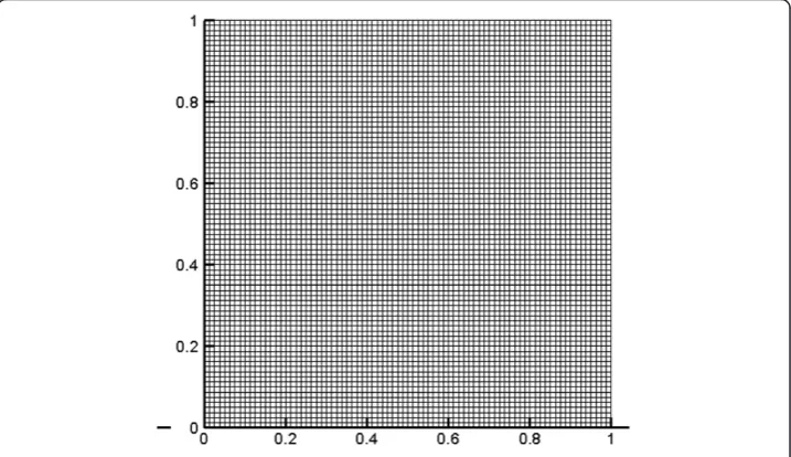
The computational example to be solved is a 0.1x0.1 m square plate with non-uniform load at the top and restrictions of movement vertically at the bottom as presented in Figure 2. This example has been extensively studied in numerical tests concerning bone remodeling algorithms [42-44]. For these values we built a mesh of 80x80 elements (see Figure 3) in the horizontal and vertical directions, respectively, and integrated these with a time step of Δt¼0:100 . The total simulation time was 200. The initial condition was λ¼1:0 and the limits used in the algorithm of bone remodeling were: 0:0125≤λ≤2:175.

The constants for the mechanical energy

For the mechanical case we used an initial Young’s modulus E0, a Poisson's modulusν

and an initial dimensionless density λ0 with values 64 MPa, 0.3 and 1.00, respectively

[44]. The dimensionless parameters of the density equation were obtained from Nack-enhorst (1997) [39,44] and weren¼2,kmec¼0:3125days1andUrefm ¼800Pa.

The mesh was produced using bilinear quadrilateral elements and four points of Gauss integration [40].

The constants for electric energy

equation, expressed as (36):

2ð Þρðρ;50KHzÞ ¼Bρm ð36Þ

Where m¼1:5486 and B¼1050:0; this is a function of the density of bone tissue.

With the aim of using dimensionless density, we multiplied and divided by ρn₀=ρn₀to

Figure 2Boundary conditions relating to bone remodeling.

produce (37):

2ð Þρð Þ ¼ρ 1050:0ρ10:5486λ

1:5486_{¼ 2ρλ}1:5486 _ð

37Þ

Where 2ρ¼1050:0ρ10:5486and depends on the initial density that considers the

com-putational model.

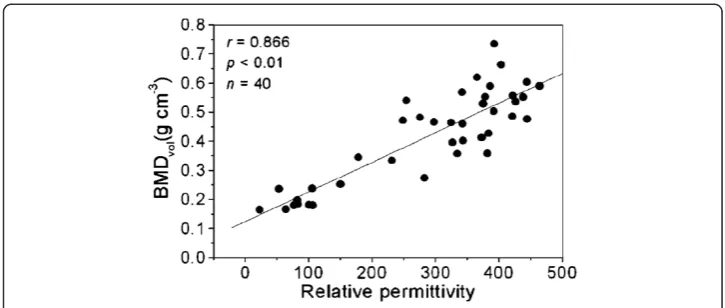
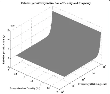
Figure 5 presents the relative permittivity in terms of the function of the frequency for the density of the femoral head ofρ¼0:3737g:cm3. With a greater frequency, per-mittivity decreases. To complement equation (37) (33) we must add a term that allows us to calculate the difference between the relative permittivity at a frequency of 50 kHz and any other frequencies used in the model; this is (38):

δð Þf ð Þ ¼ 2f r fð Þð0:3737g:cm3;fÞ 2rð50KhzÞð0:3737g:cm3;f ¼50KhzÞ

δð Þf ð Þ ¼ 2f r fð Þð0:3737g:cm3;fÞ 228:681 ð

38Þ

where 2rð50KhzÞð0:3737g:cm3;f ¼50KhzÞ ¼228:681 . For its part, the function Figure 4Bone density as a function of the relative permittivity at a frequency of 50 KHz.Taken from [46].

2r fð Þð0:3737g:cm3;fÞcan be obtained from Figure 5, so we get: log₁₀ 2r fð Þ 0:3737g:cm3;f

¼0:1407 log10ð Þf

2_{1:8936 log}

10ð Þf

þ8:1505 ð39Þ

In summary, the equation for the electric permittivity depending on the density and frequency is given by (see Figure 6):

2rðρ;fÞ ¼ 2ρλ1:5486þ 2r fð Þ228:681 ð40Þ

For the remaining constant changes we made variations of kelec and used Urefe ¼

800Pa, as in the mechanical case.

Results

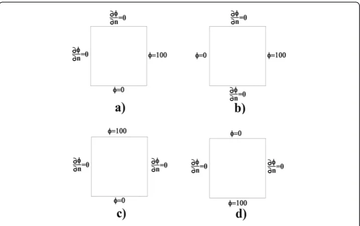
Figure 7 presents various examples that were run for a frequency f = 50 KHz, and with variation in the constant Kelect. For these examples, a potential difference at various

contour lines was imposed, according to the domain that was established in Figure 2. In the first example, a voltage of 100 was placed on the right side and no voltage at the bottom (Figure 7a). In the second example, a voltage of 100 V was placed on the right side and no voltage on the left (Figure 7b). In the third and fourth examples, the volt-age was placed on the top and bottom, respectively (Figures 7c and 7d). In the other contours we placed null Neumann conditions.

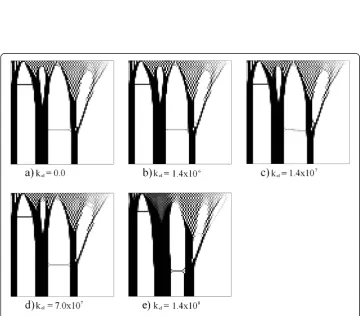
In the first example, the mechanical condition demonstrated in Figure 2 coupled with an electric field as observed in Figure 7a were used. The results are presented in Figure 8.

Figure 8 presents the results for the relative density value of λ using an approach based on element, with an average at an elementary level of the mechanical stimulus, electrical and density values. In all figures (Figures 8, 9, 10, 11 and 12) black represents the maximum density value (2,175) and white represents the lowest value (0.0125). It

Figure 7Examples developed in the article;ϕindicates voltage.

Figure 9Results for the second example: varying the frequency in equations (35) and (36).

should be noted that withΔt = 0.1 the pattern obtained is similar for all values ofkelect.

It is observed that near the area of imposition of the mechanical stress there is a similar density distribution to a chess board, and far from the loading area there is the forma-tion of three well-defined columns reminiscent of the cortical bone (Figure 8a and 8b). In cases where the constant increases (kelect= 1.4x107 and above) there is the

appear-ance of a high density area in the lower right region, from where a new column starts in the top domain (Figs 8c, d, e and f ). In this area, near the lower right structure, there is the distribution and space formation of a chess board. In addition, in the upper part there are empty areas that generate ramifications in each of the columns supporting the load. Note that the imposition of the electric field defines a new topological struc-ture in the domain, as presented on the right-hand side of the simulation results. This new structure is an additional column, which is generated by the potential and a sup-port area of higher density in the lower right corner.

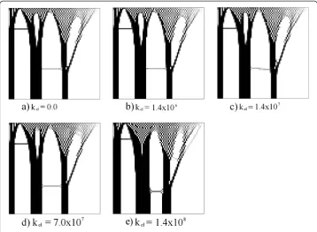
Figure 9 presents the results for various values of Kelect. In this case, a voltage of

100 V was imposed on the right side and a null voltage on the left side. Null Neumann conditions were imposed on remaining contours (see Figure 7b). It is noted that there were changes in topology; columns 2 and 3, from left to right in Figures 9c and 9d, are thicker and closer to one another. In addition, upper branches of greater density were created and an additional branch that begins from the last column to the right. In the case of Figure 9e, the formation of a non-defined region of the "chessboard" type on the right side of the domain is presented.

Figures 10 and 11 present results for various values of kelect. In these cases a voltage

of 100 V was imposed at the top and bottom, respectively. Null Neumann conditions

were imposed on the remaining contours. Note that in these cases the mass distribu-tion increases as kelect increases. In the case of Figure 10e, the density increases in the

upper part of the domain, so that the chessboard becomes more continuous in the cen-tral part of the domain. In Figures 10e and 11e the columns that are formed in each simulation have higher bandwidths than previous cases.

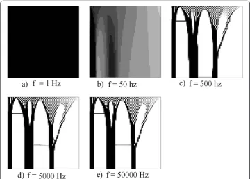
In the second example there is a variation of the frequency, while the value of kelect

remains constant at 7.0x107. With the voltage configuration of Figure 7d, this is with a lower voltage of 100 V. Note in this case that at low frequencies the density and the amount of tissue deposited are greater than at high values. Figure 9a demonstrates that the frequency generates a total deposit of tissue. In figure 12b the formation of a high density topology and continuing formation is apparent. Figures 12c, 12d and 12e present results comparable to those observed in previous cases. However, in figure 12c, the columns are wider than in figures 12d and 12e.

Discussion and conclusions

In this article several numerical examples were developed concerning bone remodeling of the plate during mechanical stress, assuming the imposition of an electric field in the domain. To calculate the mechanical and electrical stimulus of remodeling, and the evolution of density, the elemental approach was utilized. This pioneering article includes the electrical effect, previously designed by Weinans et al. [4], in a model of bone remodeling.

Comparable with previous articles, the results of the study presented herein dem-onstrate in the mechanical case formation of the columnar zone (of high density)

in the area remote from the load and formation of the trabecular zone (of low density) in the area close to the load [17]. The results are similar to those obtained by Weinans et al. [4], Fernandez et al. [49] and Chen et al. [17]. When applying an electric field there is an increase in bone density and an alteration in the top-ology of the distribution of mass in the domain. In general, there is greater bone mass apposition in the domain. Therefore, the columns developed by the mechan-ical stress increase in size due to the electric field. In addition, a greater number of columns and localized compact zones may be observed. In the formulation the effect of electrical frequency has been included to allow increased apposition of mass at low frequency to be observed.

Competing interests

The authors have no competing interests.

Acknowledgements

This work was financially supported by Division de Investigación de Bogotá, of Universidad Nacional de Colombia, under the modality: Fortalecimiento a grupos de investigación y creación artística con proyección nacional. ALIANZAS DE GRUPOS. The Project title is“Programa para la obtención y validación de parámetros numéricos utilizados en modelos matemáticos y simulación de sistemas y procesos biológicos mediante el diseño y caracterización de modelos celulares in vitro_”, Hermes code 12873.

Author details

1

Research Group on Numerical Methods for Engineering (GNUM), Universidad Nacional de Colombia, Bogota, Colombia.2_{Central University Bioengineering Group, Universidad Central de Colombia, Bogota, Colombia.}3_Biomimetics Laboratory. Biotechnonology Institute, Universidad Nacional de Colombia, Bogota, Colombia.

Authors’contributions

Work concerning production of the manuscript, modelling and numerical simulation was carried out by each of the authors. All authors read and approved the final manuscript.

Received: 24 February 2012 Accepted: 11 May 2012 Published: 11 May 2012

References

1. Ganong WF, William F:Fisiologia Médica. Mexico DF: Editorial El Manual Moderno; 2006:373–386. 2. Cowin SC:Bone mechanics handbook. Washington: CRC Press; 2001.

3. Jacobs CR, Simo JC, Beaupre GS, Carter DR:Adaptive bone remodeling incorporating simultaneous density and anisotropy considerations.J Biomech1997,30:603_–613.

4. Weinans H, Huiskes R, Grootenboer H:The behavior of adaptive bone-remodeling simulation models. J Biomech1992,25:1425_–1441.

5. Wolff J:Das Gesetz der Transformation der Knochen. Berlin: Hirschwald; 1892:1–139. 6. Frost HM:The laws of bone structure. Springfield, IL: CC Thomas; 1964.

7. Frost HM:Mathematical elements of lamellar bone remodeling. Springfield, IL: Thomas; 1964.

8. Frost HM:Vital biomechanics: proposed general concepts for skeletal adaptations to mechanical usage.Calcif Tissue Int1988,42:145–156.

9. Pauwels F:Gesammelte Abhandlungen Zur Funktionellen anatomie Des Bewegungsapparates. Berlin: Springer-Verlag; 1965:543–549.

10. Kummer B:Biomechanics of bone: mechanical properties, functional structure, functional adaptation. In

Biomechanics: its Foundations and Objectives. Edited by Fung YC, Perrone N, Anliker M. Englewood Cliffs: Prentice-Hall; 1972:237_–272.

11. Cowin S:Wolffís law of trabecular architecture at remodeling equilibrium.J Biomech Eng1986,108:83. 12. Cowin S, Hegedus D:Bone remodeling I: theory of adaptive elasticity.J Elast1976,6:313_–326.

13. Cowin S, Nachlinger RR:Bone remodeling III: uniqueness and stability in adaptive elasticity theory.J Elast1978,

8:285_–295.

14. Hegedus D, Cowin S:Bone remodeling II: small strain adaptive elasticity.J Elast1976,6:337–352.

15. Gupta S, New AMR, Taylor M:Bone remodelling inside a cemented resurfaced femoral head.Clin Biomech2006,

21:594–602.

16. Stülpner M, Reddy B, Starke G, Spirakis A:A three-dimensional finite analysis of adaptive remodelling in the proximal femur.J Biomech1997,30:1063–1066.

17. Jonkers I,et al:Relation between subject-specific hip joint loading, stress distribution in the proximal femur and bone mineral density changes after total hip replacement.J Biomech2008,41:3405–3413.

18. García J, Doblaré M, Cegoñino J:Bone remodelling simulation: a tool for implant design.Comput Mater Sci

2002,25:100–114.

19. Lian Z,et al:Effect of bone to implant contact percentage on bone remodelling surrounding a dental implant.Int J Oral Maxillofacial Surgery2010,39:690–698.

21. Hernandez C, Hazelwood S, Martin R:The relationship between basic multicellular unit activation and origination in cancellous bone.Bone1999,25:585–587.

22. Taylor D, Tilmans A:Stress intensity variations in bone microcracks during the repair process.J Theor Biol2004,

229:169–177.

23. Hernandez C, Beaupre G, Carter D:A theoretical analysis of the changes in basic multicellular unit activity at menopause.Bone2003,32:357–363.

24. Peterson MC, Riggs MM:A physiologically based mathematical model of integrated calcium homeostasis and bone remodeling.Bone2010,46:49–63.

25. Buenzli PR, Pivonka P, Smith DW:Spatio-temporal structure of cell distribution in cortical Bone Multicellular Units: a mathematical model.Bone2010,48(4):918–926.

26. Ramtani S:Electro-mechanics of bone remodelling.Int J Eng Sci2008,46:1173–1182.

27. Demiray H, Dost S:The effect of quadrupole on bone remodeling.Int J Eng Sci1996,34:257–268. 28. Fukada E, Yasuda I:On the piezoelectric effect of bone.J. Phys. Soc. Japan1957,12:1158–1162.

29. Aschero G, Gizdulich P, Mango F, Romano S:Converse piezoelectric effect detected in fresh cow femur bone* 1.J Biomech1996,29:1169–1174.

30. Beck BR, Qin Y, Rubin C, McLeod K, Otter M:The Relationship of Streaming Potential Magnitude To Strain and Periosteal Modeling 567.Med & Sci Sports & Exercise1997,29:98.

31. Gross D, Williams WS:Streaming potential and the electromechanical response of physiologically-moist bone. J Biomech1982,15:277–295.

32. Hung C, Allen F, Pollack S, Brighton C:What is the role of the convective current density in the real-time calcium response of cultured bone cells to fluid flow?J Biomech1996,29:1403–1409.

33. Johnson MW, Chakkalakal DA, Harper RA, Katz JL:Comparison of the electromechanical effects in wet and dry bone.J Biomech1980,13:437–442.

34. Qu CY, Yu SW:The damage and healing of bone in the disuse state under mechanical and electro-magnetic loadings.Procedia Engineering2011,10:171–176.

35. WANG E, ZHAO M:Regulation of tissue repair and regeneration by electric fields.Chinese Journal of Traumatology (English Edition)2010,13:55–61.

36. Demiray H:Electro-mechanical remodelling of bones.Int J Eng Sci1983,21:1117–1126.

37. Huang CP, Chen XM, Chen ZQ:Osteocyte: the impresario in the electrical stimulation for bone fracture healing.Medical hypotheses2008,70:287–290.

38. Qu C, Qin QH, Kang Y:A hypothetical mechanism of bone remodeling and modeling under electromagnetic loads.Biomaterials2006,27:4050–4057.

39. Nackenhorst U:Numerical simulation of stress stimulated bone remodeling.Tech Mech1997,17:31–40. 40. Oñate, E.Structural analysis with the finite element method. Linear statics, (Springer Verlag, 2009). 41. Hoffman JD:Numerical methods for engineers and scientists. New York: Mc Graw-Hill; 1992.

42. Beaupre G, Orr T, Carter D:An approach for time dependent bone modeling and remodelingótheoretical development.J Orthop Res1990,8:651–661.

43. Jacobs CR, Levenston ME, Beaupré GS, Simo JC, Carter DR:Numerical instabilities in bone remodeling simulations: the advantages of a node-based finite element approach.J Biomech1995,28:449–459. 44. Chen G, Pettet G, Pearcy M, McElwain D:Comparison of two numerical approaches for bone remodelling.

Medical engineering & physics2007,29:134–139.

45. Sierpowska J,et al:Prediction of mechanical properties of human trabecular bone by electrical measurements.Physiol Meas2005,26:S119.

46. Sierpowska J,et al:Electrical and dielectric properties of bovine trabecular boneórelationships with mechanical properties and mineral density.Phys Med Biol2003,48:775.

47. Gabriel C, Gabriel S, Corthout E:The dielectric properties of biological tissues: I. Literature survey.Phys Med Biol

1996,41:2231.

48. Sierpowska J,et al:Interrelationships between electrical properties and microstructure of human trabecular bone.Phys Med Biol2006,51:5289.

49. Fernández J, García-Aznar J, Martínez R, Viaño J:Numerical analysis of a strain-adaptive bone remodelling problem.Comput Methods Applied Mech Eng2010,199:1549–1557.

doi:10.1186/1742-4682-9-14

Cite this article as:Garzón-Alvaradoet al.:Numerical test concerning bone mass apposition under electrical and mechanical stimulus.Theoretical Biology and Medical Modelling20129:14.

Submit your next manuscript to BioMed Central and take full advantage of:

• Convenient online submission

• Thorough peer review

• No space constraints or color figure charges

• Immediate publication on acceptance

• Inclusion in PubMed, CAS, Scopus and Google Scholar

• Research which is freely available for redistribution