www.nat-hazards-earth-syst-sci.net/12/3719/2012/ doi:10.5194/nhess-12-3719-2012
© Author(s) 2012. CC Attribution 3.0 License.
and Earth
System Sciences
Improving probabilistic flood forecasting through a data
assimilation scheme based on genetic programming
L. Mediero, L. Garrote, and A. Chavez-Jimenez
Technical University of Madrid, Department of Civil Engineering, Hydraulic and Energy Engineering, Madrid, Spain
Correspondence to: L. Mediero ([email protected])
Received: 16 November 2011 – Revised: 28 June 2012 – Accepted: 18 September 2012 – Published: 19 December 2012
Abstract. Opportunities offered by high performance com-puting provide a significant degree of promise in the en-hancement of the performance of real-time flood forecast-ing systems. In this paper, a real-time framework for prob-abilistic flood forecasting through data assimilation is pre-sented. The distributed rainfall-runoff real-time interactive basin simulator (RIBS) model is selected to simulate the hy-drological process in the basin. Although the RIBS model is deterministic, it is run in a probabilistic way through the re-sults of calibration developed in a previous work performed by the authors that identifies the probability distribution func-tions that best characterise the most relevant model parame-ters. Adaptive techniques improve the result of flood fore-casts because the model can be adapted to observations in real time as new information is available. The new adaptive forecast model based on genetic programming as a data as-similation technique is compared with the previously devel-oped flood forecast model based on the calibration results. Both models are probabilistic as they generate an ensem-ble of hydrographs, taking the different uncertainties inherent in any forecast process into account. The Manzanares River basin was selected as a case study, with the process being computationally intensive as it requires simulation of many replicas of the ensemble in real time.
1 Introduction
Hydrological flood forecasting entails estimation of a hy-drological variable in the future from the available data in the present and the set of recorded data of flood events in the past, giving its time of occurrence, quantitative measure and reliability (Sz¨oll¨osi-Nagy, 2009). The utility of a hydro-logical forecast increases, given that its uncertainty is better
quantified either by a probability distribution of occurrence or by an ensemble of possible scenarios. Uncertainty bounds must be defined (with the potential adverse consequences) to assist flood managers and users so that they can make deci-sions taking risk into account (Komma et al., 2007).
Information about historic flood events in the past is not sufficient to fully characterise the hydrological behaviour of the basin in the future. In addition, a fixed model with con-stant parameters will not be able to represent completely the complex processes in the basin. For practical purposes, an adaptive forecast scheme may be used to adjust model pa-rameters, state variables and/or specify results of changes in the basin behaviour that cannot be simulated by the initial model setup (Young, 2002). Adaptive forecasting techniques have been applied to forecasting water levels in the River Severn in the United Kingdom (Romanowicz et al., 2006); forecasting floods in regulated basins in Korea, therefore im-proving the forecast of the high-flow events (Shamir et al., 2010); improving flood forecasts in the Rhine and Meuse rivers (Weerts et al., 2010); and improving streamflow fore-casts in France, mainly for small basins (Thirel et al., 2010). Data assimilation techniques can be used to develop an adaptive forecast model, as they update estimates of system states or parameters quantifying errors in both the hydrologi-cal model and observations. Therefore, data assimilation can improve flood forecasts (Vrugt et al., 2006). Furthermore, data assimilation applied to a distributed hydrological model has significant potential, as model estimates of basin states can be improved from observations at a gauged station keep-ing their distribution in space (Liu and Gupta, 2007; Clark et al., 2008).
were based on the Kalman filter (KF) technique (Kalman, 1960), which is used to update the model state variables from the assimilation of observed discharge data, extending the model and observed data uncertainties to uncertainties in the forecast (Bras and Rodriguez-Iturbe, 1985; Awwad and Vald´es, 1992).
The extended Kalman filter (EKF) linearises the error co-variance equation and propagates the coco-variance matrix in the future. Although it is effective in many cases, it is unsta-ble if the nonlinearities are strong and it fails in representing the error probability (Reichle and Koster, 2003). To solve this unstable behaviour, a filter based on Monte-Carlo simula-tions has been developed, termed the ensemble Kalman filter (EnKF) (Evensen, 2003, 2004), which generates an ensemble of forecasts from a set of model states that take model and observed data uncertainties into account. The model is up-dated with the variance of the ensemble prediction from dif-ferences between each ensemble member and the ensemble mean. EnKF has been widely applied as a result of recent in-creases in computing capacity, making the approach afford-able (Pauwels and De Lannoy, 2006; Shamir et al., 2010).
Kalman filters assume that the prior distribution of model states is represented by a Gaussian distribution, though state variables in hydrology do not always follow a Gaussian dis-tribution. Particle filter (PF) techniques do not assume any prior distribution, at the expense of requiring a larger num-ber of ensembles. PF assigns a probability to each ensemble element by a weight calculated as the difference between the ensemble element and the observations (Moradkhani et al., 2005; Weerts and El Serafy, 2006). Furthermore, Kalman fil-ters assume that the model paramefil-ters are known prior to the forecast. This is not the case for hydrological forecasts, how-ever, as rainfall-runoff models use parameters that represent either physical or conceptual properties of runoff processes that cannot be accurately estimated and model outputs highly depend on these parameters. Moreover, some model param-eters may not be stationary because the basin can change its behaviour during a given flood event, with data assimilation techniques being able to change its estimate of model param-eters in real time.
Genetic programming (GP) is a suitable technique in adapting model parameters to observations, given that it is designed to identify and enhance good individuals from an ensemble by applying selection and crossover techniques. GP is an evolutionary algorithm (EA), which includes a set of techniques inspired by biological evolution that simulate the evolution of individuals by means of different perturba-tions and a fitness function, such as the following: (a) genetic algorithms used to solve optimisation problems (Holland, 1975); (b) evolutionary programming (that is very similar to GP but uses a fixed structure of the problem) (Fogel et al., 1966); (c) evolution strategy that works with vectors or real numbers and uses self-adaptive mutation rates (Schwefel, 1981); (d) GP that work with trees; and (e) Neuroevolution
that uses artificial neural networks to represent the variables (Angeline, 1994).
GP uses the Darwinian natural selection principle of sur-vival and reproduction of the best individuals (from an ini-tial population the best individuals are selected with a fitness function) (Koza, 1992). These so-called better individuals are chosen to breed the next generation, applying certain pertur-bations. The new individuals fight to survive in the next gen-eration, with the process being repeated based on perturba-tions to create diversity and selection to improve the fitness (Eiben and Smith, 2007).
GP has been used in hydrology in a diversity of appli-cations. For example, a GP system was used to discover rainfall-runoff relationships in different basins from daily time series of rainfall-runoff data and a lumped model based on the unit hydrograph technique. The GP model led to a more robust model than the conventional ones (especially when surface runoff processes and precipitation losses were not correctly understood) (Whigham and Crapper, 2001). A data-driven model based on GP was developed from hydrom-eteorological data to avoid the problem of collecting data of physically-based models and to overcome the problem of formulating traditional models to describe the non-linear processes of runoff generation (Babovic and Keijzer, 2002). Both were successful approaches and improved the conven-tional models.
Khatibi et al. (2011) compared three artificial intelligence techniques to simulate the discharge routing process: artifi-cial neural networks (ANN), adaptive neuro-fuzzy inference system (ANFIS) and GP. The latter showed an improved per-formance in most of the assessment measures. Elshorbagy et al. (2010a and b) compared seven data-driven techniques in a modelling experiment: ANN, GP, evolutionary polyno-mial regression, support vector machines, M5 model trees, K-nearest neighbours and multiple-linear regression. GP was also the most successful technique in terms of predictive ac-curacy and uncertainties due to its ability to adapt the model to the data. In addition, Wang et al. (2009a) conducted a com-parison to forecast monthly discharge time series, where the GP and ANFIS models obtained the better results, though the former achieved the best forecast results in the validation phase.
1999; Wang et al., 2009b). In addition to the aforementioned cases, the GP technique was also applied to real-time fore-casting (Khu et al., 2001; Kisi and Shiri, 2011).
This paper presents the development of an adaptive flood forecast model. A sequential data assimilation technique is developed to update the estimation of the probability distri-bution of several parameters of a distributed rainfall-runoff model. The stochastic parameter estimation is performed by application of a GP algorithm to minimise the expected value of model errors. The paper is organised as follows: Sect. 2 presents the methodology to develop the adaptive flood fore-cast model; Sect. 3 introduces the case study used to test the model; Sect. 4 is devoted to discuss the results of the model in a set of flood events; and finally, the conclusions are pre-sented in Sect. 5.
2 Methodology
A hydrological forecast model estimates the response of a basin from the current observations and predictions of future meteorological conditions. As new observations are available in real time, this information can be used to update the model by data assimilation techniques. This paper focuses on the evaluation of the benefits of a data assimilation technique based on GP from a forecast without data assimilation.
This section is organised in five parts. First the rainfall-runoff model is presented, then the forecast scheme without data assimilation is described and finally the proposed fore-cast scheme with data assimilation is introduced.
2.1 Rainfall-runoff model
The methodology is applied to the real-time interactive basin simulator (RIBS) model (Garrote and Bras, 1995a and b). Such a model is composed of a runoff-generation module that estimates the infiltration capacity and obtains the evo-lution of the saturated area of the basin, as well as a flow routing module that propagates discharge across the basin. Two processes are represented in the runoff-generation mod-ule: local infiltration and lateral moisture fluxes. It is assumed that the saturated hydraulic conductivity (Ks)decreases with soil depth (z) following an exponential function. The soil is considered anisotropic, withKsvarying in directions normal (n)and parallel (p) to the sloped soil surface according to the following equations:
Ksn(z)=K0ne −f z
θ−θ
r
θs−θr
ε
(1)
Ksp(z)=K0pe
−f z θ−θr
θs−θr
ε
, (2)
whereK0n and K0p (mm h−1)are the saturated hydraulic
surface conductivities in directions normal and parallel to the surface;f (mm−1)a parameter that controls the reduction of
saturated hydraulic conductivity with depth;θthe soil mois-ture content;θrthe residual soil moisture content;θs the sat-urated moisture content; andεthe index of soil porosity.
The saturated hydraulic surface conductivities in the par-allel and normal directions are related by the anisotropy co-efficient (a):
a=K0p
K0n
. (3)
Under the kinematic approximation, the contribution of capillary forces to pore pressure is neglected (Beven, 1984). This leads to the establishment of a wetting front: a sharp discontinuity that separates two areas with different moisture content; the upper zone contains the moisture wave of the storm and the lower zone remains with the initial soil mois-ture content. The depth of the wetting front is represented by the variableNf(mm). If saturation is reached, there is also an
upper front representing the ascension of the saturated zone,
Nt (mm). Normal flow in this area,qn(mm h−1), is given by
qn=K0n
f (Nf−Nt)
ef Nf−ef Nt. (4)
Surface runoff will occur when the value of rainfall inten-sity exceeds the infiltration capacity of the soil, or when the soil is saturated.
The flow routing module simulates the runoff propagation process through the basin. Flow routing is based on the dis-tributed convolution equation:
Q(t )=
Z
A t
Z
0
Rf(x, y, τ ) h (x, y, t−τ ) dτ dA, (5)
where Q(t ) is the resulting hydrograph at the outlet,
Rf(x, y, t )is a function describing the distribution of runoff
rate generation per unit area and h(x, y, t ) is the instanta-neous response function of the element of area dA located at coordinates (x,y). The estimation of the instantaneous re-sponse function is based on travel time along the flow path, assuming constant velocities on the hillslopes (vh)and on the riverbeds (vs). To account for possible non-linearities, stream velocity,vs, may grow with the relative value of flow at the discharge point of the basin,Q(t ), with respect to a reference flow rateQref, with the exponentr:
vs(t )=Cv
Q(t ) Qref
r
. (6)
If the exponent is taken as equal to 0, vs is constant throughout the simulation. Forr >0, the channel velocity is greater than the parameterCv(m s−1)when the discharge at the outlet is above the reference value and otherwise smaller thanCv. Hillslope velocity is defined as a function of stream velocity through a dimensionless parameter,Kv:
vh(t )=
vs(t )
Kv
2.2 Forecast without data assimilation
The forecast model without data assimilation does not take advantage of the possibilities to adapt its parameters to dis-charge observations in real time, as it is based on the results of a calibration process developed prior to the occurrence of the event. However, it is formulated as an ensemble forecast to take the forecast uncertainty into account. Ensemble mod-els were developed to assess the forecast uncertainty with a low number of simulations and have shown their advantages over other techniques for operational forecasting (Rebora et al., 2006; Dietrich et al., 2009).
Forecast ensemble members are generated by sampling from the probability distributions of relevant model param-eters. The probabilistic calibration developed by Mediero et al. (2011) was applied to obtain the initial estimation of the probability distribution of model parameters. This approach was selected as it takes into account that hydrological mod-els are unable to provide a unique combination of parameters that correctly simulate all situations that may occur in the basin due to: (a) the presence of structural errors (Wagener et al., 2004); (b) a set of multiple parameters leading to an in-terval of forecast discharges that provides a better assessment of the forecast uncertainties (Beven, 2006); and (c) address-ing of the uncertainty involved in the forecast beaddress-ing crucial (Taramasso et al., 2005).
2.2.1 Probabilistic calibration
The probabilistic calibration of the RIBS rainfall-runoff model in the Manzanares River basin was carried out in Me-diero et al. (2011). A summary of this calibration is presented in this section.
The model calibration started with a sensitivity analysis of the RIBS model parameters to find the most influential pa-rameters on model results in order to reduce the number of parameters used in the calibration process. Three parameters were identified as the most influential on the model results: parameterf, which represents the variation of hydraulic con-ductivity with respect to depth; parameterKv, which repre-sents the ratio between flow velocity and hillslope velocity in the riverbed; and parameterCv, which represents a coef-ficient of the law that simulates the relationship between ve-locity on the riverbed and discharge at the outlet of the basin. Then, a set of objective functions were selected to assess the most important aspects of the hydrograph in a flood fore-cast. The hydrograph was divided into two parts according to the mean flow value: P at the end of the objective function means the upper part, and B the lower part. Four objective functions were selected: the shape of the hydrograph in its upper part analysed by the root mean squared error applied to the upper part of the hydrograph (RMSE-P); the magnitude of low flows analysed by the mean absolute error applied to its lower part (MAE-B); the utility of the hydrograph as a forecast analysed by the Nash-Sutcliffe efficiency coefficient
(NSE); and the time of occurrence of the peak analysed by the time to peak (TP) objective function.
A multi-objective calibration of the model was performed to find the set of parameter combinations that lead to the most accurate solutions, based on the Pareto solutions calculated as the set of non-dominated optimal solutions. The multi-objective calibration entailed three steps. In the first step, the Pareto solutions were obtained with the four selected objec-tive functions to identify the range of values ofCvthat leads to an accurate simulated peak time. In the second, the Pareto solutions were obtained from RMSE-P, MAE-B and NSE, identifying the parameter combinations that lead to an ac-curate simulation of the upper part of the hydrograph. And in the third, the solutions obtained in the second step that fall outside the validity range ofCvobtained in the first step were eliminated. Finally, the solutions that properly simulate the shape and peak time simultaneously were identified as calibration results with ranges that are physically meaning-ful.
A distribution function is fitted to the resulting populations of each parameter. A beta function was fitted to the logarith-mic values of parameterf:
log10(f ) = −3.15 + 2.85 × fbeta(α=2.43, β=1.75)
. (8)
ParameterKvwas represented by a Weibull function with parametersα=8.82 andβ=7.78. ParameterCvwas repre-sented by a normal distribution function with a mean (µ) of 1.883 and a standard deviation (σ) of 0.097. Independence between parameters was studied and it was found that in-dependence between parameters can be assumed. Therefore, the result of the calibration process is a set of parameter com-binations randomised from these fitted functions; that is to say, the calibration result is a probability density function for each parameter instead of a unique solution.
2.2.2 Forecast model
This first forecast model does not use data assimilation tech-niques, ignoring the new discharge observations in real-time. The model is fixed prior to the forecast from the result of the probabilistic calibration and cannot adapt itself to changes in the basin response or to forecast errors.
rainfall up to current time and then run into the future with alternative rainfall forecasts from different sources. A large fraction of model uncertainty is linked to uncertainties in the forecast rainfall. Testing the validity of these rainfall fore-casts is beyond the scope of this paper, given that the aim is testing the hydrological forecast models, not the rainfall forecasts. Therefore, the forecast model was used in hind-cast mode, assuming perfect knowledge of future rainfall, al-though emulating real-time operation. Other sources of un-certainty, such as those corresponding to the choice of initial condition, cannot be eliminated without data assimilation. 2.3 Forecast with data assimilation
The second forecast model is based on the application of GP as a data assimilation technique to adapt the model to new observations during the flood event in order to improve the first flood forecast model.
The forecast model based on GP takes the result of the cal-ibration process and the initial condition used in the forecast model without assimilation as a starting point and adapts the individuals of this first population of parameters with the new available records in each operational time step. Although the comparison between models was conducted with the same initial population, it could also be conducted with two differ-ent randomisations from the result of the probabilistic cali-bration without any significant influence on the comparison results. The data assimilation scheme is based on updating model parameter values, and therefore only one initial basin state was considered. A similar approach could be applied taking several basin states as initial condition. This approach was not considered to allow for a better comparison with re-spect to the forecast without data assimilation, where the full ensemble of model parameters was used, but only one initial basin state. The procedure used by the forecast model based on GP can be summarised as follows:
1. Generation of an initial population of parameter com-binations from a randomisation with the results of the probabilistic calibration.
2. Running of the RIBS model with this initial population of parameters in the first time step, taking the observed rainfall in this first time step as an input and obtaining an ensemble of simulations as an output.
3. Quantifying the ability to reproduce the observed hy-drograph of each individual of the ensemble population by an objective function that evaluates the fit between simulated and observed discharges.
4. Selection of the set of best individuals or parameter combinations of the ensemble from the results of the previous step. These individuals will live in the next time step and are termed the mating population.
5. Mating of the selected individuals of the ensemble, ap-plying the crossover technique or exchange of parame-ter values between them.
6. Mating of the selected individuals of the ensemble, ap-plying the mutation technique or random perturbation of the parameter values of an individual.
7. Creation of the next generation of individuals or chil-dren, joining the mating population or selected param-eter combinations in step four and the result of the crossover in step five and the result of the mutation in step six.
8. Repetition of steps two to seven up to the end of the hydrograph, taking the ensemble population of model parameters obtained in the step seven as initial popula-tion.
The steps of selection (two through four), crossover (five) and mutation (six) are described in detail as follows. 2.3.1 Selection
Selection consists of identifying the best individuals that will survive in the next generation. An individual or parameter combination is better than another when the former leads to a better representation of the observed hydrograph than the latter. Therefore, a probability to survive the next generation is assigned to each parameter combination from its ability to represent the hydrological response of the basin. The pa-rameter combinations are evaluated, punishing the papa-rameter combinations and basin states that lead to less accurate re-sults and rewarding the parameter combinations and basin states that lead to better results. The ability of an individ-ual is evaluated by an objective function. A fitness ranking was selected to assign the survival probability and parame-ter combinations are sorted by their values of the objective function. The root mean squared error (RMSE) was selected as an objective function as it gives a higher penalty to higher errors:
RMSE(θi)=
v u u t
1
N
N
X
t=1
yt−yt0(θi)
2
, (9)
whereyt is the observed flow at timet,yt0(θi)is the
simu-lated flow at timetwith parametersθi, withibeing thei-th
simulation, andNthe number of time steps used in the eval-uation, which in this case is equal to eight, as an evaluation period of two hours is used.
The selected individuals are the parents that mate and pro-duce the children in the next generation by crossover and mu-tation processes.
2.3.2 Crossover
(a)
(b)
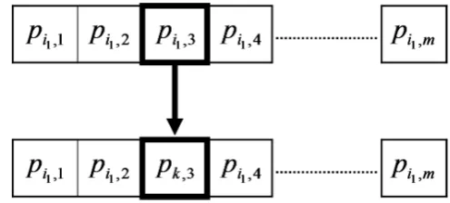
Fig. 1. Scheme of the crossover process: (a) parents; (b) children.
or parameter values between two parents. The new children inherit the parameter values of their two parents, though they do not have exactly the same characteristics as either of them, given that a genetic exchanging occurs in the process. The crossover process follows the principle that part of the offspring obtained by mating two individuals with different characteristics will improve the properties of their parents, while the rest will have worse properties than their parents. Natural selection is responsible for selecting the better in-dividuals and improving the quality of the next generation. The improved offspring will then have a higher probability of surviving the next generation.
Crossover is based on a stochastic process (Fig. 1). From the ensemble of model parameter combinations,pi,j, where
i isi-th ensemble simulation and j isj-th model parame-ter, withmthe number of model parameters, two parameter combinations are taken randomly from the ensemble (i1and
i2 in the example shown in Fig. 1). Then, a model parame-ter is selected randomly from themmodel parameters (the third parameter in the example shown in Fig. 1). The param-eter value of the first paramparam-eter combination (pi1,3)is inter-changed with the parameter value of the second parameter combination (pi2,3).
The crossover process is not always successful. The com-bination of model parameter values has to be run on a basin state which was obtained with a different parameter set. The soil moisture profile as described through the kinematic ap-proximation is unique for a given set of state variables, front positions and moisture content, and depends on model pa-rameters (in particular, on parameter f). If parameter val-ues are changed maintaining the state variable valval-ues (front position and moisture content) this could lead to numerical
Fig. 2. Scheme of the mutation process. Model parameters for the parent at the top and model parameters for the child at the bottom.
instabilities in some cells, especially in those where the top front is close to the surface, because the moisture profile can-not be adapted to the new parameter values. Such instances were simply discarded in the GP data assimilation scheme. 2.3.3 Mutation
The mutation process is based on a random change in the ge-netic material or parameter values of one individual to pro-duce a modified mutant child. Such mutation adds a pertur-bation in the parameter values of some individuals. This pro-cess differs from the crossover in that the mutation creates new parameter values, while crossover only interchanges the existing parameter values. Mutation tries to avoid the sur-vival population being highly conditioned by the observa-tions, despite the possible existence of errors in observations or changes in the basin response.
Mutation is also a stochastic process (Fig. 2). First, an en-semble individual is randomly selected from the parent pop-ulation (i1in the case of Fig. 2). Then, a model parameter is randomly taken from the mmodel parameters (pi1,3in the example shown in Fig. 2). Finally, perturbations in the value of the model parameter of that individual are produced to obtain the mutated child (pk,3). For the sake of simplicity, as small perturbation magnitudes around the initial parame-ter value are generated, perturbations are simulated by a ran-dom normal distributionN (0, σ )instead of utilising the dis-tribution functions found as result of the calibration process (Eq. 9).
fN(x)=
1
σ
√ 2πexp
"
− x 2
2σ2
#
(10) wherex is the value of the parameter andσ is the standard deviation.
values of parameters. Theσvalue for each parameter should be of a sufficient magnitude to give flexibility to the forecast model, while small enough to avoid higher uncertainties. A sensitivity analysis is conducted to fix theσ values.
2.4 Measures for testing the forecast performance
The comparison of each forecast needs certain measures that quantify the bias, accuracy and uncertainty of the forecast re-sults. Two such measures were selected to validate the fore-casts. The bias of the results was quantified by a modifica-tion of the Nash-Sutcliffe efficiency (NSE(y˜0)) coefficient that compares the utility of the median of the forecasts with that of the temporal mean of the observations (y)¯ NSE(y˜0):
NSE y˜0
=1.0−
N
P
t=1
yt− ˜yt0
2
N
P
t=1 [yt− ¯y]2
, (11)
wherey˜t0is the forecast median or value with a probability of 0.5 at timet. NSE(y˜0)has an optimal value of 1.0; a value of 0 indicates that a forecast using the mean of the observation for all time steps will have the same utility as the result of the forecast; and values below 0 indicate results are worse than the prognosis by the mean of the medians.
The accuracy of the results was quantified by the inclusion coefficient [CR(α)], which assess the ability of the model to include observed flow values within the prediction intervals of forecasts associated with a confidence levelαby calcu-lating the proportion of time intervals in which the observed flow falls within the prediction interval over the total number of time intervals (Montanari, 2005):
CR(α)=
N
P
t=1
I[yt]
N , (12)
whereI[yt]is 1 if the observed flow value falls within the
prediction interval at timet, and is 0 otherwise.
The uncertainty of the model was quantified by the coeffi-cient of variation (CV) of forecasts at each time step, which measures the dispersion of results. A lower dispersion is pre-ferred, as the forecast increases its precision.
2.5 Setup of the forecast models
Both forecast models have the following characteristics. The size of the forecast ensemble (Ne)is 100 simulations. The time step length of RIBS model run (1tr) is 15 min, as it was found to be the optimum time resolution by Atencia et al. (2011). The time step length of the simulation (1ts)and forecasting (1tf)loops is two hours. The observed rainfall is considered as forecast rainfall.
The forecast model with data assimilation has further char-acteristics. For each time step of the simulation loop, natural
Fig. 3. Location of the Manzanares River basin. Circles are stream-flow gauge stations, from north to south: Santillana reservoir, El Pardo reservoir and Rivas Vaciamadrid. Squares are precipitation gauge stations. The figure in the upper right corner represents the basin location within Spain.
selection is applied by means of the selection process. The survival rate was fixed at 50 %; hence, 50 individuals will live and 50 will die from each generation. The number of se-lected individuals (Ns)is fixed at 50. To keep the size of the forecast ensemble at 100, 50 new individuals are generated each time step by crossover and mutation by the same rate. The number of new individuals created by crossover (Nc)is 25 and the number of new individuals created by mutation (Nm)is 25.
3 Case study
The Manzanares River basin was selected as a case study. The river is located in the centre of Spain and crosses the city of Madrid (Fig. 3), having a basin area of 1248 km2. The basin outlet was taken at the gauging station Rivas Vacia-madrid, as it is located very close to its confluence with the Jarama River.
Table 1. Flood events in the Manzanares River basin.
Event Maximum Maximum Rainfall Flow intensity intensity volume volume (mm/15 min) (mm/30 min) (hm3) (hm3)
14 April 2003 5.50 9.40 20.91 1.71 5 December 2003 3.60 5.40 28.42 4.40 21 February 2004 2.20 4.40 23.23 6.80 28 April 2004 5.20 9.80 13.76 3.12
outflow discharge relative to the inflow should increase with reservoir level (Gir´on, 1988).
The Manzanares River basin has a Mediterranean climate with a wet period from autumn to spring and a dry period in summer. Therefore, most of flood events occur during the wet period. The time of concentration of the Manzanares River basin is 22 h. However, the city of Madrid is located down-stream the El Pardo reservoir, being the time of concentration of this subbasin equal to eight hours.
Maps of runoff and slope directions were generated from a digital elevation model (DEM) of 100-m cell width. The DEM was generated from maps with a horizontal scale of 1:250 000 and elevation resolution of 1 m.
Spatially distributed rainfall events were characterised from data recorded at 18 rainfall gauging stations that be-long to the SAIH network; seven are located within the basin of the Manzanares River, and the other 11 are in surround-ing areas within its area of influence. Spatial distribution of rainfall was estimated by the inverse distance weighted inter-polation method, which uses the weighted sum of the rainfall observed at gauge stations in terms of the inverse of distance to known points. Flow data were recorded in three gauging stations located in the Manzanares River: the Santillana and El Pardo dams and the Rivas Vaciamadrid station. The com-parison between both forecast models was focused on the observed discharges recorded at the outlet, for the sake of simplicity. Four flood events were considered and the corre-sponding main characteristics are shown in Table 1.
4 Results
4.1 Sensitivity analysis on the variation of mutation perturbations
The mutation process is simulated by random perturbations, with a magnitude sampled from a normal distribution. Per-turbation dispersion is fixed for each parameter byσ. A sen-sitivity analysis is carried out to fix aσvalue for each param-eter so that dispersions are big enough to provide flexibility to the forecast model, while small enough to avoid higher un-certainties. In addition, theσ parameter of the perturbations used in the mutation process gives the mutation magnitude or magnitude of parameter changes around its initial value. As these changes are slight in comparison with the parameter
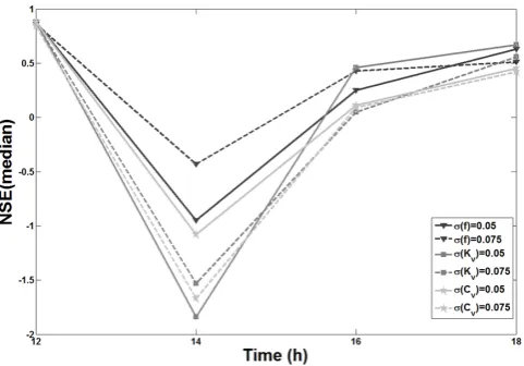
Fig. 4. Comparison of forecast model results by the NSE(y˜0)for different dispersion in the mutation process.
Table 2. Results of the NSE(y˜0)for different dispersion in the mu-tation process.
Forecast t=12 h t=14 h t=16 h t=18 h σ (f )=0.05 0.88 −0.95 0.25 0.63 σ (f )=0.075 0.86 −0.43 0.43 0.51 σ (Kv)=0.05 0.88 −1.84 0.46 0.67 σ (Kv)=0.075 0.87 −1.53 0.05 0.56 σ (Cv)=0.05 0.88 −1.08 0.11 0.45 σ (Cv)=0.075 0.84 −1.67 0.09 0.42
ranges obtained in the calibration process, a different distri-bution function from that used in the calibration can be ac-cepted.
For the following forecasting time step the RIBS model is run with the new parameter set, though starting from a basin state obtained with the parent parameter set. Since moisture profiles correspond to different parameter values from those applied in the new simulation, a large change of parameter values may lead to instabilities in the resolution of differ-ential equations of the RIBS model, and thereforeσ values were limited to 0.1. Moreover, given that values higher than 0.1 lead to very high dispersion, influence ofσ equal to 0.05 and 0.075 in forecast results was tested. The sensitivity anal-ysis entailed running the forecast model with data assimila-tion, applying the mutation process to only one of the model parameters, fixingσ for this model parameter and settingσ
equal to zero for the other two parameters. The flood event that occurred in February 2004 was selected to conduct the sensitivity analysis. The results are shown in Table 2 and Fig. 4.
L. Mediero et al.: Improving probabilistic flood forecasting through a data assimilation scheme 3727
36 a)
1
2
3
b) 4
5
6
c) 7
8
(a)
36 a)
1
2
3
b) 4
5
6
c) 7
8
(b)
36 2
3
b) 4
5
6
c) 7
8
(c)
d) 1
2
3
Figure 5. Results of the forecast models for the April 2003 flood event. The vertical dashed 4
line is the current time step. Forecasts are expressed by the median and the prediction limits 5
for a confidence level of 5%. The first column shows the results of the forecast model without 6
data assimilation and the second column the forecast model with data assimilation. The rows 7
show forecasts by current time step: a) t=29 hours; b) t=31 hours; c) t=33 hours; c) t=35 8
hours. 9
10
(d)
Fig. 5. Results of the forecast models for the April 2003 flood event. The vertical dashed line is the current time step. Forecasts are ex-pressed by the median and the prediction limits for a confidence level of 5 %. The first column shows the results of the forecast model without data assimilation and the second column the forecast model with data assimilation. The rows show forecasts by current time step: (a)t=29 h; (b)t=31 h; (c)t=33 h; (d)t=35 h.
beginning. By comparing the results of thef parameter for bothσvalues it can be seen that aσvalue equal to 0.05 only slightly improves the forecast in the last time step (t=18 h) when the peak has passed and the forecast is less important. Therefore, a dispersion given by aσ value equal to 0.075 is selected for thef parameter.
Regarding theKvparameter, there are no significant dif-ferences between the σ values in the first two time steps. However, aσ value of 0.05 gives better results at the time of peak, with an improvement of 0.40 in the NSE(y˜0). Aσ
38 a)
1
2
3
b) 4
5
6
c) 7
8
(a)
38 a)
1
2
3
b) 4
5
6
c) 7
8
(b)
38 2
3
b) 4
5
6
c) 7
8
(c)
Fig. 6. Results of the forecast models for the December 2003 flood event. The vertical dashed line is the current time step. Forecasts are expressed by the median and the prediction limits for a confi-dence level of 5 %. The first column shows the results of the forecast model without data assimilation and the second column the forecast model with data assimilation. The rows show forecasts by current time step: (a)t=16 h; (b)t=18 h; (c)t=20 h.
value of 0.05 is selected to represent the dispersion in the mutation step for theKvparameter.Cvparameter shows bet-ter results for aσ value of 0.05 in all time steps, so thisσ is selected to represent the dispersion of mutations.
4.2 Forecast improvement by data assimilation
Once mutation dispersion was fixed for each model param-eter, improvement of the forecast model with data assimila-tion based on GP over the model without data assimilaassimila-tion was assessed. The models were compared in four observed events.
4.2.1 The April 2003 flood event
Table 3. Results of the validation measures for the April 2003 flood event.
Forecast t=129 h t=131 h t=133 h t=135 h
Forecast without data assimilation
NSE(y˜0) 0.82 −0.12 −1.26 −2.19
CR (α=5) 1.00 1.00 1.00 1.00
CV 0.49 0.60 0.59 0.48
Forecast with data assimilation
NSE(y˜0) 0.74 0.54 –1.14 –1.57
CR (α=5) 1.00 1.00 1.00 1.00
CV 0.44 0.45 0.29 0.22
rainfall could be used to quantify the ability of each parame-ter combination to reproduce the observed hydrograph.
The bias of both models was measured by the NSE(y˜0). It can be seen that its results in the first time step are sim-ilar for each model. However, the forecast model with data assimilation improves the results of the model without data assimilation in the next time steps in terms of bias. In the last two time steps both models have negative values of the NSE(y˜0), as they give discharges higher than observations.
The accuracy of the models is similar from the results of the CR for a confidence level of 5 % (CR(α=5)). It can be seen that the observed hydrograph lies between the predic-tion limits for the given confidence level in all time steps.
A notable difference between the models can be seen in terms of dispersion. A significant reduction in the uncertainty of the forecast is achieved by the GP model in all time steps, as the CV is reduced up to half in the last time steps. The data assimilation technique is able to reduce the dispersion of the forecast, discarding the parameter combinations that yield worse results and selecting the parameter combinations that yield results more similar to the observations. This means that the data assimilation technique is able to reproduce the observed hydrograph during the flood event.
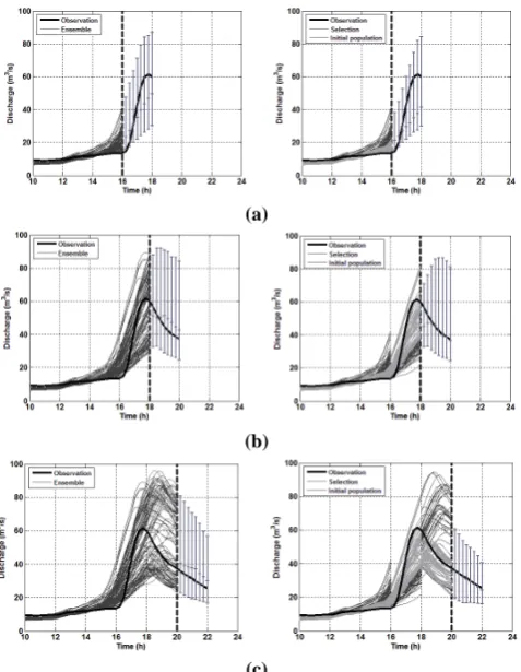
4.2.2 The December 2003 flood event
In the December 2003 flood event, the models were ini-tialised at time step 10 h and the first forecast was made at time step 16 h (Table 4 and Fig. 6). In this case, the fore-cast model based on GP obtains the best results in the last time step in terms of bias. However, the models have similar results in terms of accuracy. The observed hydrograph lies between the prediction intervals in all time steps, except at the beginning of the first time step where the models cannot be adapted to the observations.
In terms of dispersion, the GP model achieves better re-sults as it has smaller values of the CV in all time steps, with the difference being higher in the last time step. It is clear that the GP model always gives smaller dispersions than the model without data assimilation, as the former tries to adapt to the observations.
40 a)
1
2
3
b) 4
5
6
c) 7
8
(a)
40 a)
1
2
3
b) 4
5
6
c) 7
8
(b)
40 a)
1
2
3
b) 4
5
6
c) 7
8
(c)
1
d) 2
3
4
Figure 7. Results of the forecast models for the February 2004 flood event. The vertical 5
dashed line is the current time step. Forecasts are expressed by the median and the prediction 6
limits for a confidence level of 5%.The first column shows the results of the forecast model 7
without data assimilation and the second column the forecast model with data assimilation. 8
The rows show forecasts by current time step: a) t=12 hours; b) t=14 hours; c) t=16 hours; d) 9
t=18 hours. 10
(d)
Fig. 7. Results of the forecast models for the February 2004 flood event. The vertical dashed line is the current time step. Forecasts are expressed by the median and the prediction limits for a confi-dence level of 5 %.The first column shows the results of the forecast model without data assimilation and the second column the forecast model with data assimilation. The rows show forecasts by current time step: (a)t=12 h; (b)t=14 h; (c)t=16 h; (d)t=18 h.
Table 4. Results of the validation measures for the December 2003 flood event.
Forecast t=16 h t=18 h t=20 h
Forecast without data assimilation
NSE(y˜0) 0.67 0.32 −1.21 CR (α=5) 0.78 1.00 1.00
CV 0.34 0.38 0.40
Forecast with data assimilation
NSE(y˜0) 0.28 0.08 0.96 CR (α=5) 0.78 1.00 1.00
CV 0.31 0.34 0.32
4.2.3 The February 2004 flood event
Each forecast model was applied to the flood event that oc-curred in February 2004 (Table 5 and Fig. 7). The models were initialised at time step eight hours and the first forecast was made at time step 12 h.
The bias of each model was measured by the NSE(y˜0). It can be seen that bias results in the first time step are similar for each model, though bias results in the second and fourth time step are better for the model without data assimilation, while the GP model has better results in the third time step. However, the accuracy of the models is similar in terms of the CR(α=5). It can be seen that the observed hydrograph lies between the prediction limits for the given confidence level, except in the last time step where the GP forecast gives somewhat overestimated results.
A notable difference in terms of dispersion can be also observed, as in the case of the previous events. A reduction in the uncertainty of the forecast is achieved by the GP model in all time steps. The difference in the first time step is very low, though it does increase in the rest of time steps up to a half in the last two time steps, with the CV of the forecast model without data assimilation being significantly higher than the forecast model based on GP.
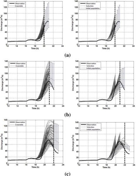
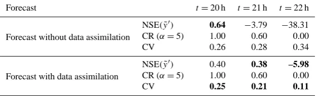
4.2.4 The April 2004 flood event
In the April 2004 flood event, the models were initialised at time step 10 h and the first forecast made at time step 20 h (Table 6 and Fig. 8).
The results show that the observation lies outside the se-lected members in some time steps. This is caused by the use of the RMSE to select the best members. This objective function gives higher penalties to higher deviations follow-ing a square law. As a result, some members that have great deviations in some time steps are discarded.
In this flood event, the bias of the GP model is better than the bias of the model without data assimilation, mainly in the last two time steps where the GP model highly improves the results. The accuracy of the models is similar in terms of the CR(α=5) and the GP improves the forecast in terms of uncertainty reduction, as in the previous cases. A notable difference in terms of dispersion can be observed, mainly in
42 a)
1
2
3
b) 4
5
6
c) 7
8
(a)
42 a)
1
2
3
b) 4
5
6
c) 7
8
(b)
42 a)
1
2
3
b) 4
5
6
c) 7
8
(c)
Fig. 8. Results of the forecast models for the April 2004 flood event. The vertical dashed line is the current time step. Forecasts are ex-pressed by the median and the prediction limits for a confidence level of 5 %. The first column shows the results of the forecast model without data assimilation and the second column the forecast model with data assimilation. The rows show forecasts by current time step: (a)t=20 h; (b)t=21 h; (c)t=22 h.
the last time step where the dispersion reduction is higher than two thirds.
5 Conclusions
Table 5. Results of the validation measures for the February 2004 flood event.
Forecast t=12 h t=14 h t=16 h t=18 h
Forecast without data assimilation
NSE(y˜0) 0.90 0.05 −1.98 0.76 CR (α=5) 1.00 1.00 1.00 1.00
CV 0.19 0.17 0.15 0.21
Forecast with data assimilation
NSE(y˜0) 0.88 −1.31 0.34 0.48 CR (α=5) 1.00 1.00 1.00 0.44
CV 0.16 0.11 0.06 0.11
Table 6. Results of the validation measures for the April 2004 flood event.
Forecast t=20 h t=21 h t=22 h
Forecast without data assimilation
NSE(y˜0) 0.64 −3.79 −38.31 CR (α=5) 1.00 0.60 0.00
CV 0.26 0.28 0.34
Forecast with data assimilation
NSE(y˜0) 0.40 0.38 –5.98
CR (α=5) 1.00 0.60 0.00
CV 0.25 0.21 0.11
with the sequential data assimilation technique presented in this paper were assessed by comparing the performance of a forecast model without data assimilation with that of a fore-cast model with data assimilation. The Manzanares River basin was selected as a case study and the RIBS model as a rainfall-runoff model. Spatially distributed observed rain-fall was used as forecast rainrain-fall in order to assess the perfor-mance of each forecast model without it being conditioned to the reliability of rainfall forecasts. In this paper, spatially distributed rainfall was estimated from data recorded at rain-fall gauging stations. However, rainrain-fall maps recorded by the radar network could be used if available. Furthermore, if new products exist, such as quantitative precipitation esti-mation or quantitative precipitation forecasts, they could be also used in the proposed forecast model.
The first forecast model, without data assimilation, was based on the results of a probabilistic calibration, which was conducted in a previous work on the selected river basin (Mediero et al., 2011). The probabilistic calibration gave as a result a probability density function for each influential pa-rameter of the RIBS model, with the aim of considering dif-ferent hydrological basin behaviours identified from the ob-served flood events. Such parameter characterisation is suit-able for flood forecasting, as the objective functions used in the calibration process were selected in order to take the most important aspects of the hydrograph for real-time flood fore-casting into account. This first forecast model does not use any assimilation technique from new observed data.
The second forecast model, with data assimilation, reduces the spread of the ensemble of the first model by using an adaptive model based on genetic programming. Data assimi-lation is conducted by three steps: a selection step to find the
parents or model parameter combinations that lead to a bet-ter fit with the observations, a crossover step to simulate the creation of new parameter combinations from interchanging parameter values between parents, and the mutation step to simulate random changes in the parameter values of parents to create new children. This forecast model takes the results of the probabilistic calibration as a starting point, though the adaptive technique is able to reproduce the observed hydro-graph and allows the model to be adapted to changes in basin response during the flood event.
The models were applied to four flood events that occurred in the Manzanares River basin. The accuracy of the mod-els is similar, as the observed hydrograph lies between the prediction limits in the majority of the time steps. Although there are further differences in terms of bias, the most im-portant improvement of the forecast model based on genetic programming was found to be in terms of dispersion or fore-cast uncertainty. The sequential model reduces the dispersion of forecasts significantly, with the dispersion being reduced by a half in most cases. It can hence be concluded that the introduction of a data assimilation scheme based on genetic programming improves the results of a forecast model based on calibration over observed events.
Acknowledgements. The authors wish to acknowledge
Edited by: N. Rebora
Reviewed by: R. Rudari, M. C. Llasat, and two anonymous referees
References
Angeline, P. J., Saunders, G. M., and Pollack, J. B.: An evolution-ary algorithm that constructs recurrent neural networks, IEEE T. Neural Networ., 5, 54–65, 1994.
Atencia, A., Mediero, L., Llasat, M. C., and Garrote, L.: Effect of radar rainfall time resolution on the predictive capability of a dis-tributed hydrologic model, Hydrol. Earth Syst. Sci., 15, 3809– 3827, doi:10.5194/hess-15-3809-2011, 2011.
Awwad, H. M. and Vald´es, J. B.: Adaptive parameter estimation for multi-site hydrologic forecasting, J. Hydraul. Eng., 118, 1201– 1221, 1992.
Aytek, A. and Alp, M.: An application of artificial intelligence for rainfall-runoff modelling, J. Earth Syst. Sci., 117, 145–155, 2008.
Babovic, V. and Keijzer, M.: Rainfall runoff modelling based on genetic programming, Nord. Hydrol., 33, 331–346, 2002. Beven, K. J.: Infiltration into a class of vertically non-uniform soils,
Hydrol. Sci. J., 29, 425–434, 1984.
Beven, K. J.: A manifesto for the equifinality thesis, J. Hydrol., 320, 18–36, 2006.
Bras, R. L. and Rodriguez-Iturbe, I.: Random functions and hydrol-ogy. Addison-Wesley, Reading, Massachusetts, USA, 1985. Cabral, M. C., Garrote, L., Bras, R. L. and Entekhabi, D.: A
kine-matic model of infiltration and runoff generation in layered and sloped soils, Adv. Water Resour., 15, 311–324, 1992.
Clark, M. P., Rupp, D. E., Woods, R. A., Zheng, X., Ibbitt, R. P., Slater, A. G. Schmidt, J., and Uddstrom, M. J.: Hydrological data assimilation with the Ensemble Kalman Filter: use of streamflow observations to update states in a distributed hydrological model, Adv. Water Resour., 31, 1309–1324, 2008.
Dietrich, J., Schumann, A. H., Redetzky, M., Walther, J., Den-hard, M., Wang, Y., Pf¨utzner, B., and B¨uttner, U.: Assessing uncertainties in flood forecasts for decision making: prototype of an operational flood management system integrating ensem-ble predictions, Nat. Hazards Earth Syst. Sci., 9, 1529–1540, doi:10.5194/nhess-9-1529-2009, 2009.
Eiben, A. E. and Smith, J. E.: Introduction to Evolutionary comput-ing. Springer, Natural Computing Series, 2007.
Elshorbagy, A., Corzo, G., Srinivasulu, S., and Solomatine, D. P.: Experimental investigation of the predictive capabilities of data driven modeling techniques in hydrology – Part 1: Con-cepts and methodology, Hydrol. Earth Syst. Sci., 14, 1931–1941, doi:10.5194/hess-14-1931-2010, 2010a.
Elshorbagy, A., Corzo, G., Srinivasulu, S., and Solomatine, D. P.: Experimental investigation of the predictive capabilities of data driven modeling techniques in hydrology – Part 2: Application, Hydrol. Earth Syst. Sci., 14, 1943–1961, doi:10.5194/hess-14-1943-2010, 2010b.
Evensen, G.: The Ensemble Kalman Filter: theoretical formula-tion and practical implementaformula-tion, Ocean Dynam., 53, 343–367, 2003.
Evensen, G.: Sampling strategies and square root analysis schemes for the EnKF, Ocean Dynam., 54, 539–560, 2004.
Fogel, L. J., Owens, A. J., and Walsh, M. J.: Artificial Intelligence through simulated evolution. John Willey, New York, 1966. Garrote, L. and Bras, R. L.: A distributed model for real-time
fore-casting using digital elevation models, J. Hydrol., 167, 279–306, 1995a.
Garrote, L. and Bras, R. L.: An integrated software environment for real-time use of a distributed hydrologic model, J. Hydrol., 167, 307–326, 1995b.
Gir´on, F.: The evacuation of floods during the operation of reser-voirs, Transactions of the Sixteenth International Congress on Large dams, vol. 4, Report 25, 403–417, Beijing, China, 1988. Holland, J. H.: Adaptation in natural and artificial systems,
Univer-sity of Michigan Press, Ann Arbor, Michigan, 1975.
Kalman, R. E.: A new approach to linear filtering and prediction problems, J. Basic Eng.-T ASME, 82, 35–45, 1960.
Khatibi, R., Ghorbani, M. A., Kashani, M. H., and Kisi, O.: Com-parison of three artificial intelligence techniques for discharge routing, J. Hydrol., 403, 201–212, 2011.
Khu, S. T., Liong, S. Y., Babovic, V., Madsen, H., and Muttil, N.: Genetic programming and its application in real-time runoff fore-casting, J. Am. Water Resour. As., 37, 439–451, 2001.
Kisi, O. and Shiri, J.: Precipitation forecasting using wavelet-genetic programming and wavelet-neuro-fuzzy conjunction models, Water Resour. Manag., 25, 3135–3152, 2011.
Komma, J., Reszler, C., Bl¨oschl, G., and Haiden, T.: Ensem-ble prediction of floods – catchment non-linearity and fore-cast probabilities, Nat. Hazards Earth Syst. Sci., 7, 431–444, doi:10.5194/nhess-7-431-2007, 2007.
Koza, J. R.: Genetic programming: on the programming of comput-ers by means of natural selection, The MIT Press, Cambridge, Massachusetts, 1992.
Liu, Y. and Gupta, H. V.: Uncertainty in hydrologic modeling: to-ward an integrated data assimilation framework, Water Resour. Res., 43, W070401, doi:10.1029/2006WR005756, 2007. Mediero, L., Garrote, L., and Mart´ın-Carrasco, F. J.: Probabilistic
calibration of a distributed hydrological model for flood forecast-ing. Hydrol. Sci. J., 56, 1129–1149, 2011.
Montanari, A.: Large sample behaviours of the generalized likeli-hood uncertainty estimation (GLUE) in assessing the uncertainty of rainfall–runoff simulations, Water Resour. Res., 41, W08406, doi:10.1029/2004WR003826, 2005.
Moradkhani, H., Hsu, K., Gupta, H. V., and Sorooshian, S.: Uncer-tainty assessment of hydrologic model states and parameters: se-quential data assimilation using the particle filter. Water Resour. Res., 41, W070401, doi:10.1029/2004WR003604, 2005. Parasuraman, K. and Elshorbagy, A.: Toward improving the
reliability of hydrologic prediction: model structure uncer-tainty and its quantification using ensemble-based genetic programming framework, Water Resour. Res., 44, W12406, doi:10.1029/2007WR006451, 2008.
Pauwels, R. N. and De Lannoy, J. M.: Improvement of modeled soil wetness conditions and turbulent fluxes through the assimilation of observe discharge, J. Hydrometeorol., 7, 458–477, 2006. Rabunal, J. R., Puertas, J., Suarez, J., and Rivero, D.: Determination
of the unit hydrograph of a typical urban basin using genetic pro-gramming and artificial neural networks, Hydrol. Process., 21, 476–485, 2007.
Mediterranean area, Nat. Hazards Earth Syst. Sci., 6, 611–619, doi:10.5194/nhess-6-611-2006, 2006.
Reichle, R. L. and Koster, R. D.: Assesing the impact of horizontal error correlations in backgorund fields on soil moisture estima-tion, J. Hydrometeorol., 3, 728–740, 2003.
Romanowicz, R. J., Young, P. C., and Beven, K. J.: Data assimila-tion and adaptive forecasting of water levels in the river Severn catchment, United Kingdom, Water Resour. Res., 42, W06407, doi:10.1029/2005WR004373, 2006.
Savic, D. A., Walters, G. A., and Davidson, J. W.: A Genetic Pro-gramming approach to rainfall-runoff modelling, Water Resour. Manag., 13, 219–231, 1999.
Schwefel, H. P.: Numerical optimization of computer models, John Wiley, Chichester, United Kingdom, 1981.
Shamir, E., Byong-Ju, L., Deg-Hyo, B., and Georgakakos, P.: Flood forecasting in regulated basins using the Ensemble Extended Kalman Filter with storage function method, J. Hydrol. Eng., 115, 1030–1044, 2010.
Sz¨oll¨osi-Nagy, A.: Learning from your errors – if you can! Reflec-tions on the value of hydrological forecasting models, UNESCO-IHE, Delft, The Netherlands, 2009.
Taramasso, A. C., Gabellani, S., and Parodi, A.: An operational flash-flood forecasting chain applied to the test cases of the EU project HYDROPTIMET, Nat. Hazards Earth Syst. Sci., 5, 703– 710, doi:10.5194/nhess-5-703-2005, 2005.
Thirel, G., Martin, E., Mahfouf, J.-F., Massart, S., Ricci, S., Regim-beau, F., and Habets, F.: A past discharge assimilation system for ensemble streamflow forecasts over France – Part 2: Impact on the ensemble streamflow forecasts, Hydrol. Earth Syst. Sci., 14, 1639–1653, doi:10.5194/hess-14-1639-2010, 2010.
Vrugt, J. A., Gupta, H. V., Nuall´ain, B. ´O., and Bouten, W.: Real-time data assimilation for operational ensemble streamflow fore-casting, J. Hydrometeorol., 7, 548–565, 2006.
Wagener, T., Wheater, H. S., and Gupta, H. V.: Rainfall–runoff mod-elling in gauged and ungauged catchments, London, Imperial College Press, 2004.
Wang, W. C., Chau, K. W., Cheng, C. T., and Qiu, L.: A comparison of performance of several artificial intelligence methods for fore-casting monthly discharge time series, J. Hydrol., 374, 294–306, 2009a.
Wang, W. C., Xu, D., Qiu, L., and Ma, J.: Genetic programming for modelling long-term hydrological time series, Fifth International Conference on Natural Computation (ICNC), 4, 265–269, 2009b. Weerts, A. H. and El Serafy, G. Y. H.: Particle filtering and ensem-ble Kalman filtering for state updating with hydrological con-ceptual rainfall-runoff models, Water Resour. Res., 42, W09403, doi:10.1029/2005WR004093, 2006.
Weerts, A. H., Serafy, G. Y., Hummel, S., Dhondia, J., and Gerrit-sen, H.: Application of generic data assimilation tools (DATools) for flood forecasting purposes, Comput. Geosci., 36, 453–463, 2010.
Whigham, P. A. and Crapper, P. F.: Modelling rainfall-runoff us-ing genetic programmus-ing, Math. Comput. Model., 33, 707–721, 2001.