www.nat-hazards-earth-syst-sci.net/11/445/2011/ doi:10.5194/nhess-11-445-2011
© Author(s) 2011. CC Attribution 3.0 License.
and Earth
System Sciences
Seismicity dynamics and earthquake predictability
G. A. Sobolev
The Schmidt Institute of Physics of the Earth, Russian Academy of Sciences, Moscow, Russia
Received: 18 October 2010 – Revised: 17 December 2010 – Accepted: 22 December 2010 – Published: 14 February 2011
Abstract. Many factors complicate earthquake sequences, including the heterogeneity and self-similarity of the geological medium, the hierarchical structure of faults and stresses, and small-scale variations in the stresses from different sources. A seismic process is a type of nonlinear dissipative system demonstrating opposing trends towards order and chaos. Transitions from equilibrium to unstable equilibrium and local dynamic instability appear when there is an inflow of energy; reverse transitions appear when energy is dissipating. Several metastable areas of a different scale exist in the seismically active region before an earthquake. Some earthquakes are preceded by precursory phenomena of a different scale in space and time. These include long-term activation, seismic quiescence, foreshocks in the broad and narrow sense, hidden periodical vibrations, effects of the synchronization of seismic activity, and others. Such phenomena indicate that the dynamic system of lithosphere is moving to a new state – catastrophe. A number of examples of medium-term and short-term precursors is shown in this paper. However, no precursors identified to date are clear and unambiguous: the percentage of missed targets and false alarms is high. The weak fluctuations from outer and internal sources play a great role on the eve of an earthquake and the occurrence time of the future event depends on the collective behavior of triggers. The main task is to improve the methods of metastable zone detection and probabilistic forecasting.
1 Introduction
Measurements of the Earth’s surface movements taken over the last 20 years using space geodetic methods have identified movements irregular in size and direction. They are most distinct along the Pacific coast, the south-eastern
Correspondence to: G. A. Sobolev ([email protected])
edge of the Indian Ocean, and the E-W belt from the Himalayas to the Mediterranean Sea. These are also regions with the most intensive seismic activity. All this leaves little doubt about the fact that the majority of earthquakes are caused by the strain process, i.e. stress accumulation due to incompatibility of strains. Facts and arguments cited in this paper refer to these earthquakes as tectonic earthquakes. The author explains his understanding of the seismic process and earthquake predictability based on 30 years of research experience in this area. It is quite possible, however, that interpretation of some experimental data can be explained in a different way because we are dealing with a very little-studied field of natural science.
22 1
2
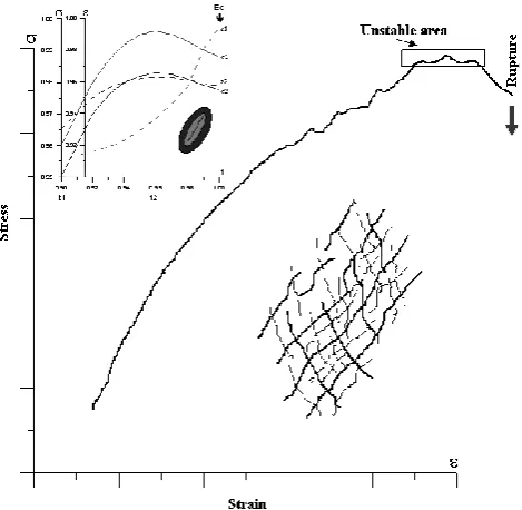
Figure 1. A rheological diagram σ-ε near the long-term strength limit: in the top left corner – the 3
process development diagram; in the bottom right corner – structure diagram of distribution of 4
blocks and faults in rock massif. Other explanations – in the text. 5
6
Fig. 1. A rheological diagramσ-εnear the long-term strength limit: in the top left corner – the process development diagram; in the bottom right corner – structure diagram of distribution of blocks and faults in rock massif. Other explanations – in the text.
1F that has resulted in instability to strainDin the process of instability development, i.e.k=1F /D. If such ratio is large, then effective stresses decrease while unstable strain is developing; therefore, macrodestruction may not occur. This was demonstrated in a series of experiments with a servo control press on which a constant strain rate is maintained. In a soft mechanism, the process is explosion-like and continues for a short period of time after the strength limit is achieved. The level of stiffness for a natural loading mechanism (plate movement) is not known. If the section where strength is decreasing (prior to an earthquake) occupies a finite interval of time, it is possible to follow the development of a seismic process up to the dynamic displacement (earthquake) to be able to predict such phenomenon.
In the top left corner in Fig. 1, one can see the process development diagram. Let us assume that stressσ1near a
fault in a certain block 1 at a certain timet1reaches the level
of 96% of failure stress. If stress continues to rise, it will, at a timet2, reach a level sufficient for development of unstable
strain, which is followed by an increase in strain rateε1 in
the near-fault area and a simultaneous drop in the level of stressσ1. Acceleration of strain in the event of brittle failure
of rock is also evident in increasing seismic activity. Let us also suppose that the level of stressσ2 at a timet1 in the
adjacent block 2 was at 95%. By the timet2, it has not risen
enough for instability to develop in this block. The loss of accumulated energy to maintain the process of unstable strain in the near-fault area in block 1 and the associated drop in stress σ1 will result in some decrease in stress in adjacent
blocks. The strain rateε2in such blocks will go down and
seismic activity will also decrease. Therefore, when unstable strain is developing in time, a rock massif is divided into two areas with different strain (and seismic) processes. One may expect that seismic activation will be developing within block 1, with seismic quiescence in the neighboring blocks.
Bak et al. (1989) introduced a concept that they termed “self-organized criticality” (SOC) in order to explain the behavior of the “sandpile” model. In the pure SOC model large earthquakes are inherently unpredictable (Geller, 1997), because any small earthquake can evolve into a strong event: thus a large event is just a small earthquake that did not stop. In another works, the heterogeneous structure of the lithosphere was taken into account. The critical point CP theory, on the contrary, has considered a large earthquake as a final result of some developing process, such as the clustering of events towards the critical concentration, coinciding with the percolation threshold. The final rupture can be predicted by monitoring the process of clustering of small faults (Chelidze, 1982). The same conclusion was reached in the case of anisotropical geometry of fracture structures (Chelidze et al., 2006). Some hybrid models appeared that integrated CP and SOC theories. A model of earthquakes on a pre-existing hierarchical fault structure was suggested in (Huang et al., 1998). The cumulative energy released by precursors follows a time-to-failure power law with log-periodic structures. Further down the hierarchy, smaller earthquakes exhibit the same phenomenology. The “self-organized critical behavior” was explained in terms of an inverse cascade of clusters and several forecasting algorithms were suggested (Newman and Turcotte, 2002). Authors of (Hainzl et al., 2000) considered a spring-block system with transient creep characteristics. Aside from a short-term increase of seismicity immediately prior to large model earthquakes, these events were preceded by an intermediate-term period of reduced seismicity (quiescence). Thus, the modern theoretical models do not exclude predictability of earthquakes.
field around such a fault changes. This idea implies an important conclusion related to earthquake predictability. A small rupture will stop at the boundary of a high strength area or adverse stress structure, which will prevent a major earthquake.
2 Main phases of seismic process prior to large earthquake
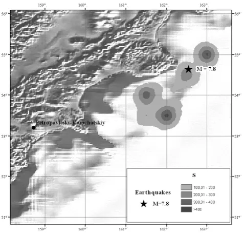
As an example, we will use the findings from the analysis of the Kronotskoe earthquake that occurred on Kamchatka on 5 December 1997 (54.64◦N–162.55◦E), with a magnitude of M=7.8. It was the most powerful earthquake within the Kamchatka seismic area during the period represented in the instrumental catalog since 1 January 1962. The catalog was compiled by the Russian Geophysical Service and is representative starting from the minimum local magnitude M >2.6. In Fig. 2, the main shock is shown as a star, aftershocks occurring over a period of 1.3 years are shown as crosses, and events three days before the earthquake are shown as circles. The latter are concentrated on a narrow area near the north-eastern edge of the earthquake rupture. We have compared the mean seismicity rate (the number of events and released seismic energy) over a period of 35 years since 1 January 1962 up to the Kronotskoe earthquake on 5 December 1997 in the area within a radius of 100 km from the epicenter of the Kronotskoe earthquake. In the first approximation, both parameters were constant over this period. If we compare this fact with the rheological curve shown in Fig. 1, we may assume that the lithosphere in the earthquake region was in an area of unstable equilibrium, with minor fluctuations in stresses.
A more thorough analysis using the RTL method (Sobolev and Tyupkin, 1997; Sobolev, 2001), with the number and energy of seismic events taken into account, made it possible to identify an area of seismic quiescence prior to the Kronotskoe earthquake. The RTL-method uses three functions (1) to measure the state of seismicity at a given location as a function of time. R(x,y,z,t ) assigns a decreasing weight to each earthquake in the catalog as a function of epicentral distance from the point of interest, T (x,y,z,t )decreases the weight of each event as a function of the difference from the time of interest, andL(x,y,z,t ) weighs the contribution to the algorithm by the rupture length of each event.
These functions are defined as R (x,y,z,t )=6exp(−ri/ro)−Rltr
T (x,y,z,t )=6exp(t−ti/t0)−Tltr
L(x,y,z,t )=6 (li/ri)p−Lltr (1)
In these formulas, x, y, z, and t are the coordinates, the depth, and time, respectively. ri is the epicentral
distance of current events from the location selected for
Fig. 2. Areal distribution of aftershocks (crosses) and foreshocks
(circles) of Kronotskoe earthquake of 5 December 1997. The star is mark the main shockM=7.8.
analyses, ti is the occurrence time of the past seismic
events, and li is the length of rupture. The Rltr, Tltr,
Lltr are the long-term averages of these functions. By
subtracting them, they eliminate the linear trends of the corresponding functions.rois a coefficient that characterizes
the diminishing influence of more distant seismic events;tois
the coefficient characterizing the rate at which the preceding seismic events are “forgotten” as the time of analysis moves on; andpis the coefficient that characterizes the contribution of size of each preceding event. With p=1, 2 or 3, this quantity is proportional to rupture length, square of rupture, or the energy, respectively. R,T andL are dimensionless functions. They are further normalized by their standard deviations, σR, σT, and σL, respectively. The product of
the above three functions is calculated as the RTL-parameter, which describes the deviation from the background level of seismicity and is in units of the standard deviation, σ = σRσTσL.
Fig. 3. Temporal variations of the RTL parameter (a) at epicenter
of the Kronotskoe and (b) at epicenter of the Simushirskoe earthquakes. The thick arrows mark the moments of these events. The thin arrows indicate the times when the reports were sent to the National Earthquake Prediction Council of the Russian Ministry Emergency Situations.
Figures 4 and 5 show that earthquakes with M∼7 are possible. From the two examples above it follows that predictability of a major earthquake in the medium-term (a few years or months before such earthquake) is not impossible but, in both cases, the magnitude of the expected earthquakes was less than that of actual events. In addition, there were areas of quiescence that did not end with major earthquakes. This can be clearly seen in Fig. 5 where anomalies were also found in other parts of the Kuril Arc, apart from the anomaly in the area of the Simushirskoe earthquake withM=8.2.
If we go back to Fig. 3, we note that in both cases in question there was a phase when the RTL curve recovered to the background level after its lowest point. Let us call this a phase of foreshock activation in a broad sense. Location of activation zones is shown in Figs. 6 and 7. We made an assumption that the rupture area, Si of the i-th event
with local magnitudeMi is proportional toEi2/3, whereEi
is the seismic energy estimated by the following empirical relations:
logEi(J)=1.5Mi+4.6 (for Kamchatka)
logEi(J)=1.3Mi+5.2 (for Kuril Arc) (2)
The value of the parameter S is equal to the difference
Fig. 4. Areas of seismic quiescence before the Kronotskoe
earthquake. The star marks the main shockM=7.8.
Fig. 5. Areas of seismic quiescence before the Simushirskoe
earthquake. The star marks the main shockM=8.2.
Fig. 6. Areas of foreshock activation before the Kronotskoe earthquake. The star marks the main shockM=7.8.
Fig. 7. Areas of foreshock activation before the Simushirskoe
earthquake. The star marks the main shockM=8.2.
Let us take a look at the changes in the seismic situation near the epicenters of the Kronotskoe and Simushirskoe earthquakes over several years preceding these events. The power law acceleration of acoustic emission before fracture and foreshocks acceleration before earthquakes as the signs of criticality was given in (Chelidze, 1982; Chelidze et al., 2006). A practical useful approach to describe possible acceleration of the seismic process prior to an earthquake was offered in (Varnes, 1989). We write the corresponding model in the form (3),
Q(t )=A−B (tf−ti)m (3)
whereQ=6i √
Ei is the accumulated Benioff strain,Ei is
29 1
2
Figure 8. Plots of Benioff strain curves Q (solid lines) and experimental values 3
(circles) for (a) the Kronotskoe and (b) Simushirskoe earthquakes. The arrows are mark the 4
moments of main shocks. 5
6
Fig. 8. Plots of Benioff strain curves Q (solid lines) and
experimental Q values (circles) for (a) the Kronotskoe and (b) Simushirskoe earthquakes. The arrows mark the moments of main shocks.
the energy of current events, tf is the time moment of the
main shock,kand 0< m <1 are model parameters, andti≤
tfis current time.
Data for the Kronotskoe earthquake have been gathered since 1994 within R=50 km from the epicenter. As can be seen in Fig. 8a, the total accumulated strain prior to the Kronotskoye earthquake followed more or less the linear law; acceleration took place three days before the main shock. In this case, the acceleration resulted from a string of earthquakes shown in Fig. 2 in circles. The exact number of days is of minor importance. What is more important is that the three-day period was much shorter than the previous interval of seismic activity, several years long, described as a linear increase in cumulative deformation (Benioff strain). The forecast timetf according to model (3) for the
Kronotskoe earthquake pointed at 25 February 1998, or 2.7 months later than the actual event.
Data for the Simushirskoe earthquake have been gathered since 2001, also within R =50 km from the epicenter. Figure 8b shows that strain accumulation occurred during 5.5 years nearly according to the linear law; acceleration took place 1.5 months before the shock. The forecast time tf according to model (3) for the Simushirskoe earthquake
30 1
2
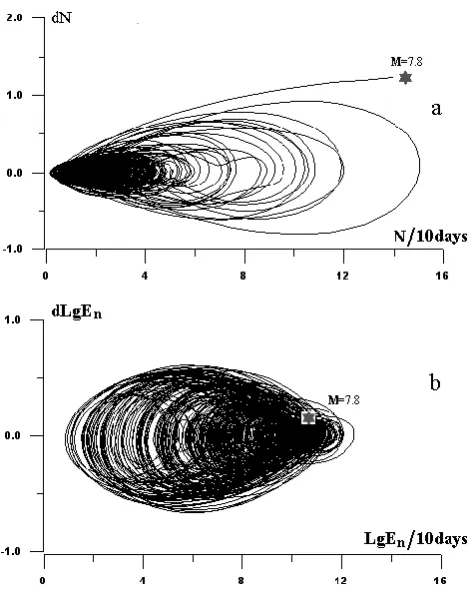
Figure 9. Phase portrait of seismicity within a radius of 100 km from the epicenter of the 3
Kronotskoe earthquake for a 35-year period (01.01.1962 – 05.12.1997). The smoothed number N 4
of earthquakes (a) or energy LgEn, Joules (b) for 10 consecutive days is marked on the X axis. 5
Rates at which these parameters change (dN or dLgEn), i.e. the difference between the following 6
and the preceding values are shown on the Y axis. The clockwise movement along the curve 7
corresponds to an increase in time. The star is mark the position of main shock. 8
Fig. 9. Phase portrait of seismicity within a radius of 100 km from
the epicenter of the Kronotskoe earthquake for a 35-year period (1 January 1962–5 December 1997). The smoothed numberN of earthquakes (a) or energy LgEn, Joules (b) for 10 consecutive days is marked on the X axis. Rates at which these parameters change (dN ordLgEn), i.e. the difference between the following and the preceding values are shown on the Y axis. The clockwise movement along the curve corresponds to an increase in time. The star marks the position of the main shock.
Fig. 8, both the Kronotskoe and Simushirskoe earthquakes were preceded by short-time seismicity activation near their epicenters. Let us consider how unique these phenomena are and whether or not they may be treated as reliable forecasting criteria.
A dynamical system may be defined as a deterministic mathematical prescription for evolving the state of a system forward in time. The dynamical system in which time t is a continuous variable could be presented as a system ofM first-order ordinary differential equations dx(t )/dt= F[x(t )], where x is M-dimensional vector. The space (x1,x2,...,xi) is referred to as phase space and the path in phase space followed by the system state as it evolves with time is referred as an orbit or trajectory. The detailed explanation of these terms can be found for example in (Ott, 2002).
Let us consider a one-dimensional space phasedN/dt= F (N ) or dLgEn/dt=F (LgEn) diagram (phase portrait) of seismicity within a radius of 100 km from the epicenter
31 1
2
Figure 10. Phase portrait of seismicity within a radius of 100 km from the epicenter of the 3
Simushirskoe earthquake for a 44-year period (01.01.1962 – 15.11.2005). The smoothed number 4
N of earthquakes for 10 consecutive days is marked on the X axis. Rates at which these 5
parameters change, i.e. the difference between the following and the preceding values are shown 6
on the Y axis. The clockwise movement along the curve corresponds to an increase in time. The 7
stars are mark the positions of main shock (M = 8.2) and foreshock (M = 5.2). 8
Fig. 10. Phase portrait of seismicity within a radius of 100 km from
the epicenter of the Simushirskoe earthquake for a 44-year period (1 January 1962–15 November 2005). The smoothed numberNof earthquakes for 10 consecutive days is marked on the X axis. Rates at which these parameters change, i.e. the difference between the following and the preceding values are shown on the Y axis. The clockwise movement along the curve corresponds to an increase in time. The stars mark the positions of the main shock (M=8.2) and foreshock (M=5.2).
of the Kronotskoe earthquake for a period starting from the beginning of the homogeneous instrumental catalog for Kamchatka (1 January 1962) unitl this earthquake on 5 December 1997, Fig. 9. The smoothed number N of earthquakes Fig. 9a or energy (LgEn, Joules) (Fig. 9b) for 10 consecutive days is marked on the X axis. Rates at which these parameters change (dN or dLgEn), i.e. the difference between the following and the preceding values marked on the X axis are shown on the Y axis. The clockwise trajectories correspond to an increase in time. They did not present in space-phase as closed lines. This is one of characteristics of a dissipative system (Nicolis and Prigogine, 1989). It is an important concept in dynamics that dissipative systems typically are characterized by the presence of attracting sets of trajectories or attractors in the phase space.
32 1
2
Figure 11. Phase portrait of seismicity within a radius of 100 km from the epicenter of the 3
Haicheng earthquake for a 5-year period (01.01.1970 – 04.02.1975). The smoothed number N of 4
earthquakes for 10 consecutive days is marked on the X axis. Rates at which these parameters 5
change, i.e. the difference between the following and the preceding values are shown on the Y 6
axis. The clockwise movement along the curve corresponds to an increase in time. The stars are 7
mark the position of main shock (M = 7.4) and foreshock (M = 5.2). 8
9
Fig. 11. Phase portrait of seismicity within a radius of 100 km
from the epicenter of the Haicheng earthquake for a 5-year period (1 January 1970–4 February 1975). The smoothed numberN of earthquakes for 10 consecutive days is marked on the X axis. Rates at which these parameters change, i.e. the difference between the following and the preceding values are shown on the Y axis. The clockwise movement along the curve corresponds to an increase in time. The stars mark the position of the main shock (M=7.4) and foreshock (M=5.2).
and state- dependent friction (Becker, 2000). This type of attractor appears when two incompatible processes are in action: loss of stable equilibrium due to energy inflow and deceleration of instability at energy dissipation or due to certain external influence. In our case, an increase in dN value means a developing instability of the seismic process while its subsequent decrease is due to loss of accumulated elastic energy when earthquakes occur or decrease in stress driven by an unknown factor. Such processes have occurred again and again in the area of the Kronotskoe earthquake in question for years, see Fig. 9. The abnormal shift of the curve dN = f(N) out of the area of the long-term attractor was brought about by a series of shocks that occurred three days before the earthquake in question (shown in Fig. 2 in circles). If we exclude these shocks from the phase portrait, the curve will remain inside the attractor. The interesting point here is that the phase portrait based on released energy data dLgEn=G(LgEn)does not show any precursor represented as a shift of the curve out of the area of the long-term attractor, which can be clearly seen in the Fig. 9b; the star that denotes the time of the earthquake is within the attractor.
The situation preceding the Simushirskoe earthquake on 15 November 2006 was somewhat different. Fig. 10 shows curves dN from 1 January 1962 till 15 November 2006. The curve dN shifted beyond the limits of the long-term attractor after the first group of foreshocks (29–30 September). A major earthquake could be expected during this period. However, there was only a moderate earthquake withM= 5.2 on 1 October. After that, the curve dN made one turn prior to the Simushirskoe earthquake. The phase portrait implies that there were abnormal shifts of dN out of the area of the long-term attractor when groups of earthquakes with magnitudes of 5–6 occurred within a radius of 100 km from the epicenter of the Simushirskoe earthquake. At the same time, there are no abnormal shifts from the long-term attractor in the curvedLgEn=f (LgEn).
The Haicheng earthquake (M=7.4) that occurred on 4 February 1975 in China (40.70◦N–122.70◦E) stands out among the other global severe earthquakes because this event was predicted in the short term and people were even evacuated (Raleigh et al., 1977; Wang, 2006). Let us take a look at its phase portrait. In doing so, we will use the seismic catalog for north-eastern China compiled by the State Seismological Bureau, China. According to our estimates, it is representative from a magnitude of M >3, starting from 1970. Over a period of 5 years, the number of shocks within a radius of 100 km from the epicenter of the Haicheng earthquake did not exceed one/day shock until 22 December 1974 when a series of 20 events took place. The curve dN shifted beyond the limits of the long-term attractor after these group of foreshocks Fig. 11. A major earthquake could be expected during this period. However, there was only a moderate earthquake withM=5.2 on 22 December. After that, the curve dN made one turn prior to the Haicheng earthquake. Reactivation occurred two days before the main shock. It consisted of 15 events; the most powerful event had a magnitude of M=5.1. The phase portrait Fig. 11 resembles the situation before the Simushirskoe earthquake Fig. 10.
We also analyzed the phase portrait of the next catas-trophic earthquake in China, the Tangshan earthquake, on 28 July 1976 (39.63◦N–118.18◦E), M=7.9, and did not find any abnormal features which would indicate the upcoming event. Note that this earthquake was not predicted. At the end of this section we would like to emphasize that the phase portrait of dN = f(N) used as a forecasting criteria is likely to be successful only if there is a series of foreshocks. Moreover, abnormal shifts from the level of the long-term attractor are observed (according to our data) before earthquake swarms with the main shocks of M <6, i.e. they do not pose any serious threat in terms of the practical use of forecasting data.
33 1
2
Figure 12. Main phases of seismic activity prior to earthquake and earthquake forecasting. 3
4
Fig. 12. Main phases of seismic activity prior to earthquake and
earthquake forecasting.
in seismicity in a relevant region in conjuction with a gradual growth of tectonic stresses. The latter, in their turn, arise at the joints of the earth’s crustal plates moving at a different rate. Let us name this period of increase in seismicity as a phase of long-term activation, Fig. 12. the spatial dimensions of a region of long-term activation before a large earthquake (M=7−8) may exceed one thousand kilometers. The above phenomena of abnormal seismic events such as seismic quiescence, foreshock activation in a broad sense are shown schematically on a diagram in Fig. 12. If we go back to Fig. 3, we note that in both cases in question there was a time delay between returning the RTL curve to the background level and main shock. This phase is also shown on a diagram together with the following phase foreshocks and triggers. We would like to note that, except for the 5 phases discussed above, sometimes also other anomalies may appear. In the paper (Scholz, 1990) additional phases were selected: a doughnut pattern was observed in the period of development of the seismic quiescence around its external limits, and seismic silence was noticed just prior to the main event.
3 Triggering effects
Let us consider some other seismic effects which may appear at different stages of development of an earthquake source representing the state of metastability. In this respect, we proceed from the following basic definitions:
– A seismic process is a type of nonlinear dissipative systems demonstrating opposed trends towards order and chaos.
– Transitions from equilibrium to unstable equilibrium and local dynamic instability appear when there is an inflow of energy; reverse transitions appear when energy is dissipating.
Phases of unstable equilibrium are manifested in such phe-nomena as stochastic oscillations and their synchronization, flicker noise, explosive noise impulses, etc. (Ott, 2002). The effect of latent periodic oscillations that appeared under four earthquakes on Kamchatka with M≥7 was found in (Sobolev, 2003). A method was used (Lyubushin et al., 1998) to identify latent periods in a point process to which an earthquake flow belongs. We considered the model of intensity of the event sequence (in the given case, the times of significant local maximums, i.e., pulsations of a microseismic time series), presumably containing a harmonic component (4)
λ(t )=µ(1+acos(ωt+ϕ)), (4)
where, the frequencyω, amplitudea, 0≤a≤1, phase angle ϕ,ϕ∈ [0,2π]and factorµ≥0, (describing the Poisson part of the intensity) are model parameters. Thus, the Poisson part of the intensity is modeled by harmonic oscillations. If a richer intensity model (compared to that for a random flow of events) with a harmonic component of a given frequency ωis considered, the associated increment in the logarithmic function of likelihood is
1lnL(a,ϕ|ω)=X ti
ln(1+acos(ωti+ϕ))
+Nln
ωT
[ωT+a (sin(ωT )+ϕ)−sin(ϕ)]
(5) hereti is the sequence of time moments of sufficiently large
local maximums of the signal within the window,N is their number, andT is the window width. Function (6)
R(ω)=max1lnL(a,ϕ|ω), 0≤a≤1, ϕ∈[0,2π] (6) may be regarded as a generalization of the spectrum for a sequence of events. The plot of this function illustrates how advantageous the periodic intensity model is in comparison with the purely random model. The maximum values of function (6) specify frequencies that are present in the flow of events. Letτ be the time of the right-hand end of the moving time window of a given widthTW. Expression (6) is
actually a function of two argumentsR(ω,τ|TW) that can be
visualized as 2-D maps on the plane of arguments (ω,τ). By using this frequency-time diagram, it is possible to examine the dynamics of the appearance and development of periodic components within the flow of the events under study.
Fig. 13. Spectral-temporal diagram of the logarithmic likelihood
function 1lnL increments for the area with a radius of 50 km around the center of the aftershock zone of the Kronotskoe earthquake of 5 December 1997. The ordinates show the spectral periods. The occurrence time of the Kronotskoe earthquake (M=
7.8) is shown by the arrow.
of the oscillation period from 0.9 years to 1.8 years (as the moment the earthquake approaches) might be interpreted as the appearance of flicker noise because one of its characteristics is the tendency towards linear (in the log-log scale) dependence of spectrum power on frequency. It is difficult to verify such dependence on the basis of a seismic catalog. A set of frequencies within the range of several orders is needed for quantitative assessment of the steepness of a spectrum dip into the high frequency (long period) range. In our case, spectrum changes are within the range of the same order.
Let us see how clearly the onset of periodic oscillations specifies the development stage of a major earthquake. Figure 14 shows a time spectrogram for 1lnL in an area with a radius of 50 km center of which shifted 100 km away to S-W from the center of the aftershock zone for the Kronotskoe earthquake. One can see that periodic oscillations within several period bands from 0.2 years to 1.2 years appeared before and after the Kronotskoye event in this region. However, what is more remarkable is that oscillations were also identified immediately after the 2006 Simushirskoe earthquake, 1000 km away from this region. It was found that at the same time periodic oscillations appeared in other, although not in all, regions of Kamchatka, i.e. the effect was selective. The onset of periodic oscillations is one of the markers showing that instability is developing in dissipative systems (Nicolis and Prigogine, 1989).
The above examples referred to the onset of periodic oscillations several years before a major earthquake; the periods were about one year long. Seismic catalogs with earthquake statistics covering dozens or even hundreds of events per year do not allow us to study this effect over a short period of time immediately before a major earthquake, which is of practical interest for short-term prediction. It appears promising to study seismic noise in order to find
Fig. 14. Spectral-temporal diagram of the logarithmic likelihood
function1lnLincrements for the area with a radius of 50 km for the region center of which shifted 100 km away from the center of the aftershock zone for the Kronotskoe earthquake. The ordinates show the spectral periods. The occurrence times of the Kronotskoe earthquake of 5 December 1997 and the Simushirskoe earthquake of 15 November 2006 (M=8.2) are shown by the arrows.
an approach to this problem. The dynamics of microseisms within a minute range of periods before several global major earthquakes was studied in (Sobolev and Lyubushin, 2007a). The records from five broadband IRIS stations were analyzed for one month before the Kronotskoe earthquake on 5 December 1997, Fig. 15. The PET station closest to the earthquake epicenter was located 350 km away while the most remote OBN station was 6800 km away. Three hours before the main shock, a clear anomaly (periods within the 25–60 min range) is observed at the PET station, closest to the epicenter Fig. 15. The beginning of the anomaly coincides with the time of the powerful foreshock with M=5.5. Records from other stations show that periodic oscillations appeared several times, e.g. two days and 15 h before the Kronotskoye earthquake; moreover, such oscillations are found at stations more than 1000 km away from each other and from the epicenter of the Kronotskoe earthquake. What is the possible reason for their appearance? We have checked two possible factors on a global scale: a source of electromagnetic emission or atmospheric disturbance. We have found that the magnetic field during the period of 2–5 December 1997 was normal (no geomagnetic storms with Kp index
greater than 3). However, a typhoon “PAKA” of the highest Category 5 developed on 2 December in the Western Pacific (http://weather.unisys.com/hurricane/); the wind speed reached 160,m h−1. One can assume that this natural phenomenon caused periodic oscillations of microseismic noise recorded by seismic stations. Typhoons generate ocean waves, which induce ground motions on the seafloor. Such processes lead to arising microsismic signals observed at far distances (Sutton and Barstow, 1996).
Fig. 15. Spectral-temporal diagrams of the logarithmic likelihood
function 1lnL increments for the microseisms recorded at the 5 different IRIS stations. The ordinates show the spectral periods. The occurrence time of the Kronotskoe earthquake of 5 December 1997, M=7.8, (54.64◦N–162.55◦E) is shown by the arrow. Coordinates of IRIS stations are: PET – (53.02◦N–158.65◦E), YAK – (62.01◦N–129.41◦E), OBN – (55.06◦N–36.34◦E), MAG – (59.34◦N–150.46◦E). YSS – (46.57◦N–142.45◦E).
various origin. In this case, it is advisable to use programs to search for synchronization intervals in records made by several stations. The spectral measure of coherence was proposed in (Lyubushin, 1998) and is based on the use of canonical coherences, which extend the notion of the spectrum of coherence to the situation where, instead of a pair of scalar time series, it is necessary to investigate the relationship between two vector time series at various frequencies: an m-dimensional series X(t ) and an n-dimensional seriesY (t ). The quantityµ21(ω), which is called the squared modulus of the first canonical coherence of the seriesX(t )andY (t )and is used in this case instead of the ordinary coherence spectrum, is calculated as the maximum eigenvalue of the matrix (Brillinger, 1975)
U (ω)=Sxx−1(ω)·Sxy(ω)·S−yy1(ω)·Syx(ω) (7)
in the discrete time enumerating successive samples. Here, ω is the frequency; Sxx(ω) is the spectral m×m matrix
of the time series X(t ); and Sxy(ω) is a cross-spectral
rectangular m×n, matrix, Syx(ω)=SxyH(ω), where the
superscriptHmeans Hermitian conjugation. The component canonical coherencesνi2(ω)of theq-dimensional time series Z(t )(q≥3)are defined as the squared moduli of the first canonical coherence if the series Y (t ) in (7) is the i-th scalar component of theq-dimensional seriesZ(t )and the seriesX(t )is the (q−1)-dimensional series consisting of the other components. Thus, the quantity νi2(ω) characterizes the correlation at the frequency ωof variations in the i-th component with variations in all of the other components. A frequency-dependent statistic λ(ω) characterizing the
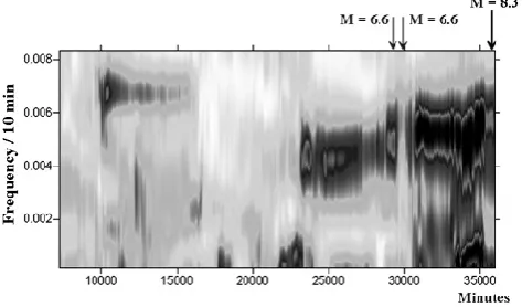
Fig. 16. Frequency-time diagram of the evolution of the
spectral measure of coherenceλ(t,ω) for seismic records of the stations YSS (46.57◦N–142.45◦E), MDJ (44.37◦N–129.35◦E), INC (37.29◦N–126.38◦E). Arrows indicate successively time moments of 2 remote earthquakes (M=6.6) and of the Hokkaido earthquake,M=8.3, (41.81◦N–143.91◦E).
correlation at the frequency ω between variations in all components of the vector seriesZ(t )is defined as:
λ(ω)= q Y
i=1
νi(ω) (8)
The example of λ(ω) analysis before the Hokkaido earth-quake of 25 September 2003,M=8.3 (41.81◦N–143.91◦E) was presented in (Sobolev and Lyubushin, 2007a). The largest number of stations participating in the computation was six: YSS, MDJ, INC, BJT, PET, OBN. It was significant that with complete sorting by 3 stations the most vivid effect was observed for stations nearest to the epicenter of Hokkaido earthquake (less than 1000 km). Spectrum-time diagram for such stations YSS, MDJ, INC is shown in Fig. 16. Three features may be noted: (1) synchronization with period∼3 h (frequency∼0.005 1 min−1) started 9 days before the earthquake (23 000 min); (2) most vividly and in a wide range of periods it was manifested 2 days before the earthquake (33 000–35 000 min); (3) a break in synchronization in the interval of 29 000–31 000 min was evidently associated with two remote strong earthquakes (shown with thin arrows) with magnitude 6.6. The first of them with the epicenter coordinates (19.72◦N– 95.46◦E) occurred on 21 September and the second one with coordinates (21.16◦N–71.67◦W) occurred 10 h later on 22 September. The brightness of this anomaly increased after these two events.
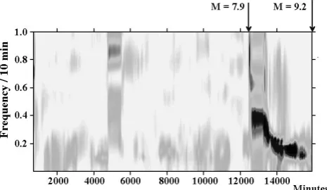
Fig. 17. Frequency-time diagrams of the evolution of the spectral measure of coherenceλ(t,ω) for seismic records of the stations XAN (34.02◦N–108.55 E), KMI (25.07◦N–102.44◦E), CHTO (18.47◦N–98.59◦E), COCO (12.11◦N–96.50◦E). Arrows indicate successively time moments of Macquarie earthquake,M=
7.9, (49.31◦S–143.91◦E) and of Sumatra earthquake, M=9.2, (3.32◦N–95.85◦E).
Southern Hemisphere withM=7.9. The epicenter of that earthquake [49.31◦S, 161.35◦E] was south-west of New Zealand (near the Macquarie Ridge). Figure 17 shows a time spectrogram for λ(ω) obtained after processing records from CHTO, KMI, XAN, COCO stations located less than 4000 km away from the epicenter of the Sumatra earthquake. After the Macquarie earthquake,λ(ω)increased while dominant periods of oscillations gradually extend from several minutes to dozens of minutes. Such an effect in the range of much longer periods was mentioned above (Fig. 13) and discussed as possible flicker noise.
Consider the following specific features of the “bursts” of oscillations that were revealed before the Kronotskoe earthquake, the Hokkaido earthquake, and the Sumatra earthquake. They appeared or increased in amplitude after disturbing effects: it was a powerful typhoon in the first case and strong earthquakes in the two other cases. Let us assume that appearance of a “burst” of periodic oscillation is a sign of instability in a seismic area. If they appear on a regular basis, this may mean that the some regions of seismoactive area are permanently in the metastable state; therefore, it is difficult to use this phenomenon for prediction purposes. If, however, they appear only before large earthquakes, this may serve as a sign of transition to dynamic instability of a potential source. Up-to-date experience suggests that the “bursts” have appeared and disappeared on more than one occasion before the same earthquake, i.e. this type of precursor is ambiguous.
4 Discussion
All this brings up the question: What is the nature of the onset of periodic oscillations and their synchronization? Let us discuss the possibilities based on the physics of
non-equilibrium systems. Let us assume that sections of a seismic area are in the metastable state prior to a strong earthquake when strain sensitivity to external exposure increases. The causes of their formation may be inside and outside the solid Earth. Processes in the outer spheres of the Earth (the atmosphere, ionosphere) are characterized by both random and quasi-periodic components. We proceed from the assumption that the dissipative system of the seismically active zone is in a meta-stable state and processes going on in it have characteristics of determined chaos. Similar systems exist in different areas of the inner and outer spheres of the Earth. If then seismicity flow (or microseisms field) reflects space and time variations of different dynamic systems parameters and non-zero coefficients of relation between parameters of these systems exist, then mutual influence by each system on another may be possible. It is well known that random systems show synchronization effects, especially in the attractors area (Ott, 2002; Pykovski et al., 2003). Synchronization of the systems dynamics may appear and be interrupted, and at some time intervals it may be stable (Gauthier and Bienfang, 1996).
In applications, random systems are frequently encoun-tered, in which the oscillations amplitude remaining finite changes in time irregularly from minimum to maximum and attractors are represented by cyclic orbits (Rossler, 1976). In such random systems, phase synchronization effects are manifested (Ott, 2002). Characteristic curve of amplitude variation against time is shown in the upper part of Fig. 18. Let Eq. (9) describe a random system affected by periodic oscillations.
dx/dt=F (x)+K·P (ωt ) (9)
Suppose we deal with oscillations in the lithosphere and coefficientK shows the extent of influence of atmospheric pressure periodic disturbances made on them. The synchronization area in the frequency band ω (Fig. 18) is characterized by the following important characteristics (Ott, 2002): it is not manifested if the relation coefficient K is less than thresholdK0; it expands asK increases. We may
assume that when an earthquake is approaching, sensitivity of the metastable section of the lithosphere (K value) to external source exposure increases. Under these conditions, dissipation impulses of the elastic energy accumulated in the lithosphere will take place at certain intervals. It is possible to detect synchronization on several frequencies if the phase locking range is wide at frequencyωs (largeK value). We
cannot rule out also the possibility when the oscillations in question occur are due to purely lithospherical reasons. The occurrence of rhythms is a common phenomenon of evolution of non-equilibrium systems (Nicolis and Prigogine, 1989).
Fig. 18. Diagram illustrating the occurrence of the synchronization
effects in a dynamic system containing chaotic and quasi-periodic components. The upper curve is an example of temporal variations in the vibration amplitude (see explanations in the text).
the degree of the mutual influence of blocks (or seismically active faults) increases as macroscopic instability (an earthquake) has been approached. This is accompanied by enlargement of the geometric region of collective behavior and in agreement with the concept of self-organized seismic criticality (Bak et al., 1989; Sornette and Sammis, 1995). In this case, the spectrum of vibrations can evolve into the lower frequency range. We realize that, to gain more substantiated ideas of the physical mechanisms responsible for the phenomena discussed in this paper, additional (and not only seismological) investigations are required.
Summing up available data and knowledge about the dynamics of a seismic process and earthquake predictability, let us take a look again at Fig. 1. Within a seismic region, there are always a few areas in the state of unstable equilibrium due to increased stress (e.g., at the ends of active faults) or reduced strength. Occurrence of dynamic instability in one such area due to external exposure (including minor fluctuations) or internal trigger effects (e.g., reduction in strength when liquid pore pressure rises) will result in a minor earthquake. Given the fractal structure of the lithosphere (areas with different strength and stress), a dynamic rupture may continue if it consistently comes across adjacent sections with unstable equilibrium. This will increase the energy (magnitude) of a developing earthquake (the domino effect). Note that occurrence of an unstable displacement in each section may, in terms of the theory of non-equilibrium dynamical systems, be referred to as bifurcation (catastrophe) while a series of bifurcations may be regarded as complex bifurcation (a system of bifurcations).
The scheme given in Fig. 1 implies the condition of predictability of a major earthquake. A researcher would like to know the following: (1) formation of a seismic region, subject to strength of blocks and faults of various
Fig. 19. A rheological diagramσ-εnear the strength limit with the loading arrangement of stick-slip experiment; the star marks the triggering shock; the large arrow marks the time of stick-slip.
scale; (2) structure of existing areas of unstable equilibrium; (3) volume of the region of relatively homogeneous tectonic stresses which will determine possible maximum length of a developing dynamical rupture. The task given under (1) may be solved by geophysical and seismic methods; the one given under (2), by analysis of minor seismicity data over a long period of time; the one given under (3), by studying focus mechanisms. Knowledge of these data is very superficial. Moreover, the time for transition to dynamic instability in the first one of the unstable equilibrium areas depends on many factors, both internal and external. It may be noted without exaggeration that the time of occurrence of all earthquakes depends on the trigger impact. Therefore, we may expect in the foreseeable future that predictions will come true with a low probability of success in determination of all three components, i.e. place, time, and magnitude.
level, the value of relative block movement, seismograms of impacts, and resulting displacements (microearthquakes). As a result, it was found that the probability of a stick-slip is proportional to the level of shear contact stress σ and impact stress f. In the first approximation, it is governed by Formula (10).
p∼σ+fn (10)
where the sum of normalized to the failure stress values |σ+f| ≤1 and a coefficientndepends on poorly known parameters of experiment.
At a low level ofσ and a smallf value, the probability of a stick-slip is close to zero. When approaching instability (a subhorizontal section of the rheological curve in Fig. 19), the probability of a dynamic displacement increases and approaches 1. However, it was revealed that a stick-slip appears with time delay 1t in relation to the moment of impact as per Formula (11), which makes prediction of time when it appears more difficult;
1t∼1fc (11)
wherec≈0.6.
It is appropriate at this point to mention the results of impact action on acoustic emission in laboratory experiments (Sobolev et al., 2001). If impacts are made on a sample similar to that given in Fig. 19 but without a cut, then (as the strength limit is approaching) the impact will result in a series of signals the number of which decreases in time according to the Omori’s law. So, the trigger impact causes a reaction similar to a series of aftershocks after a strong earthquake.
It is evident that it remotely resembles a natural situation in a seismic area. The probability of successful prediction of an earthquake will increase when we improve our knowledge about the stressed state of active faults and the force of impact on such faults by internal and external factors. The interaction of cracks was the key stone of avalanche-like model for earthquake forerunners (Mjachkin et al., 1975). The number of works in this field is rapidly increasing (Gomberg and Davis, 1996; Harris and Day, 1993; Hill, 2008; Scholz, 2010). The quasi-static interaction is modeled using the Coulomb failure function. Dynamic interaction may predominate over the quasi-static interaction at large distances (Felzer and Brodsky, 2006). However, dynamic stress changes caused by seismic waves interacting with the active faults of different type and size are little known.
5 Conclusions
The following objective conditions shall be taken into account when developing earthquake predictability studies. No precursors identified to date are clear and unambiguous: the percentage of missed targets and false alarms is high. Such ambiguity is caused by: (a) the “internal” reason, i.e. the random nature of a catastrophe against the background
of minor fluctuations in parameters of a heterogeneous dissipative system of the lithosphere; (b) the “external” reason, i.e. lack of our knowledge about the properties of such system.
The time of earthquakes is determined by the trigger impact. In this paper, we did not give examples of other precursors such as geophysical, hydrological precursors, etc. However, these is ample evidence accumulated by researchers in various seismic areas to prove their ambiguity and low reliability concerning prediction of a certain earthquake (Wyss, 1997; Cicerone et al., 2009).
Given the above, the following steps towards predictability look reasonable: (a) determine the volume of an unstable area (systems of local unstable areas of various scales); (b) monitor the trigger effects and assess their impact on unstable areas; (c) estimate of probability (reasonable, not high) of the place, time, and magnitude of an earthquake.
Acknowledgements. The author is grateful to the reviewers for
very useful comments.
Edited by: K. Eftaxias
Reviewed by: T. Nagao and another anonymous referee
References
Bak, P., Tang, S., and Winsenfeld, K.: Earthquakes as self-organized critical phenomenon, J. Geophys. Res., 94, 15635– 15637, 1989.
Becker, T. W.: Deterministic chaos in two state-variable friction sliders and the effect of elastic interactions, in: GeoComplexity and the Physics of Earthquakes, edited by: Rundle, J. B., Turcotte, D. L., and Klein, W., Geoph. Monog. Series, 120, 5–26, 2000.
Brillinger, D. R.: Time series. Data analysis and theory, Holt, Rinehart and Winston, New York, USA, 479 pp., 1975. Chelidze, T.: Percolation and fracture, Phys. Earth Planet. In., 28,
93–101, 1982.
Chelidze, T., Kolesnikov, Yu., and Matcharashvili, T.: Seis-mological criticality concept and percolation model of frac-ture, Geophys. J. Int., 164, 125–136, doi:10.1111/j.1365-246X.2005.02818.x, 2006.
Cicerone, R. D., Ebel, J. E., and Britton, J.: A systematic compilation of earthquake precursors, Tectonophysics, 476, 371–396, 2009.
Felzer, K. R. and Brodsky, E. E.: Decay of aftershock density with distance indicates triggering by dynamic stress, Nature, 441, 735–738, 2006.
Gauthier, D. J. and Bienfang, J. C.: Intermittent loss of synchronization in coupled chaotic oscillators : Towards a new criterion for high quality synchronization, Phys. Rev. Lett., 77, 1751–1759, 1996.
Geller, R.: Earthquake prediction: a critical review, Geophys. J. Int., 131, 425–450, 1997.
Hainzl, S., Zoller, G., Kurths, J., and Zschau, J.: Seismic quiescence as an indicator for large earthquakes in a system of self-organized criticality, Geophys. Res. Lett., 27(5), 597–600, 2000.
Harris, R. A. and Day, S. M.: Dynamics of fault interaction: parallel strike-slip faults, J. Geophys. Res., 98, 4461–4472, 1993. Hill, D. P.: Dynamic stresses, Coulomb failure, and remote
triggering, B. Seismol. Soc. Am., 98(1), 66–92, 2008.
Huang, Y., Saleur, H., Sammis, C., and Sornette, D.: Precursors, aftershocks, criticality and self-organized criticality, EPL-Europhys. Lett., 41, 43–48, 1998.
Huang, Q., Sobolev, G., and Nagao, T.: Characteristics of seismic quiescence and activation patterns before the M = 7.2 Kobe earthquake, January 17, 1995, Tectonophysics, 337, 99–116, 2001.
Lyubushin, A. A.: Analysis of canonical coherences in the problems of geophysical monitoring, Izvestiya Phys. Solid Earth, 34, 52– 58, 1998.
Lyubushin, A. A., Pisarenko, V. F., Ruzich, V. V., and Buddo, V. Yu.: A new method for identifying seismicity periodicities, Volcanology and Seismology, 20, 73–89, 1998.
Mjachkin, V. I., Brace, W. F., Sobolev, G. A., and Dieterich, J. H.: Two models for earthquake forerunners, Pure Appl. Geophys., 113, 169–181, 1975.
Newman, W. I. and Turcotte, D. L.: A simple model for the earthquake cycle combining self-organized complexity with critical point behavior, Nonlin. Processes Geophys., 9, 453–461, doi:10.5194/npg-9-453-2002, 2002.
Nicolis, G. and Prigogine, I.: Exploring Complexity. An introduction, W.H.Freeman and Company, New York, USA, 328 pp., 1989.
Ouilion, G., Castaing, C., and Sornette, D.: Hierarchical geometry of faulting, J. Geophys. Res., 101, 5477–5487, 1996.
Ott, E.: Chaos in dynamic systems, Cambridge University Press, 478 pp., 2002.
Power, W. L. and Tullis, T. E.: A review of the fractal character of natural fault surfaces with implications for friction and the evolution of fault zones, in: Fractals in The Earth Sciences, edited by: Lapointe, P. and Barton, C., Plenum, New York, USA, 89–105, 1995.
Pykovsky, A., Rosenblum, M., and Kurths, J.: Synchronization: A universal concept in nonlinear science, Cambridge Univ. Press, 478 pp., 2003.
Raleigh, C. B., Bennett, G., Craig, H., Hanks, T., Molnar, P., Nur, A., Savage, J., Scholz, C., Turner, R., and Wu, F.: Prediction of the Haicheng earthquake, EOS T. Am. Geophys. Un., 72, 236– 272, 1977.
Rossler, O. E.: An equation for continuous chaos, Phys. Lett. A, 57, 397–399, 1976.
Scholz, C. H.: The mechanics of earthquakes and faulting, Cambridge Univ. Press, 439 pp., 1990.
Scholz, C. H.: Large earthquake triggering, clustering, and the synchronization of faults, B. Seismol. Soc. Am., 100(3), 901– 909, 2010.
Sobolev, G.: The examples of earthquake preparation in Kamchatka and Japan, Tectonophysics, 338, 269–279, 2001.
Sobolev, G. A.: Evolution of periodic variations in the seismic intensity before strong earthquakes, Izvestiya Phys. Solid Earth, 39(11), 873–884, 2003.
Sobolev, G. A. and Lyubushin, A. A.: Using modern seismological data to reveal earthquake precursors, Russ. J. Earth. Sci., 9, ES2005, doi:10.2205/2007ES000220, 2007a.
Sobolev, G. A. and Lyubushin, A. A.: Microseismic anomalies before the Sumatra earthquake of December 26, 2004, Izvestiya Phys. Solid Earth, 43(5), 341–353, 2007b.
Sobolev, G. A. and Tyupkin, Y. S.: Low-seismicity precursors of large earthquakes in Kamchatka, Volcanology and Seismology, 18, 433–446, 1997.
Sobolev, G., Spetzler, H., Koltsov, A., and Chelidze, T.: An experimental study of triggered stick-slip, Pure Appl. Geophys., 140(1), 79–94, 1993.
Sobolev, G. A., Ponomarev, A. V., Kol’tsov, A. V., Salov, B. G., Babichev, O. V., Terent’ev, V. A., Patonin, A. V., and Mostryukov, A. O.: Excitation of acoustic emission by elastic impulses, Izvestiya Phys. Solid Earth, 37(1), 73–77, 2001. Sobolev, G. A., Valeev, S. G., and Faskhutdinova, V. A.:
Multihar-monic model of seismic activity in Kamchatka, Izvestiya Phys. Solid Earth, 46(12), 1019–1034, 2010.
Sornette, D. and Sammis, C. G.: Complex critical exponents from renormalization group theory of earthquakes: implications for earthquake predictions, J. Phys. I France, 5, 607–619, 1995. Stakhovsky, I. R.: Self-similar seismogenic structure of the crust: a
review of the problem and a mathematical model, Izvestiya Phys. Solid Earth, 43(12), 1012–1023, 2007.
Sutton, G. H. and Barstow, N.: Ocean bottom microseisms from a distant supertyphoon, Geophys. Res. Lett., 23, 499–502, 1996. Varnes, D. J.: Predicting earthquakes by analyzing accelerating
precursory seismic activity, Pure Appl. Geophys., 130, 661–686, 1989.
Wang, A. D.: Predicting the 1975 Haicheng earthquake, B. Seismol. Soc. Am., 96(3), 757–795, 2006.
Wyss, M.: Second round of evaluations of proposed earthquake precursors, Pure Appl. Geophys., 149, 169–181, 1997.