R E S E A R C H
Open Access
Dynamically analyzing cell interactions in
biological environments using multiagent
social learning framework
Chengwei Zhang
1, Xiaohong Li
1*, Shuxin Li
1and Zhiyong Feng
2FromBiological Ontologies and Knowledge bases workshop on IEEE BIBM 2016 Shenzhen, China.16 December 2016
Abstract
Background: Biological environment is uncertain and its dynamic is similar to the multiagent environment, thus the research results of the multiagent system area can provide valuable insights to the understanding of biology and are of great significance for the study of biology. Learning in a multiagent environment is highly dynamic since the environment is not stationary anymore and each agent’s behavior changes adaptively in response to other coexisting learners, and vice versa. The dynamics becomes more unpredictable when we move from fixed-agent interaction environments to multiagent social learning framework. Analytical understanding of the underlying dynamics is important and challenging.
Results: In this work, we present a social learning framework with homogeneous learners (e.g., Policy Hill Climbing (PHC) learners), and model the behavior of players in the social learning framework as a hybrid dynamical system. By analyzing the dynamical system, we obtain some conditions about convergence or non-convergence. We
experimentally verify the predictive power of our model using a number of representative games. Experimental results confirm the theoretical analysis.
Conclusion: Under multiagent social learning framework, we modeled the behavior of agent in biologic
environment, and theoretically analyzed the dynamics of the model. We present some sufficient conditions about convergence or non-convergence and prove them theoretically. It can be used to predict the convergence of the system.
Keywords: Multiagent learning, Cell interaction, Nonlinear dynamic
Background
All living systems live in environments that are uncertain and dynamically-changing. However, it is remarkable that these systems survive and achieve their goals by exhibiting intelligent features such as adaption and robustness. Bio-logical system behaviors [1] and human diseases [2] are often the outcome of complex interactions among a very large number of cells and their environments [3, 4].
*Correspondence: [email protected]
1School of Computer Science and Technology, Tianjin University, Peiyang Park
Campus: No.135 Yaguan Road, Haihe Education Park, 300350 Tianjin, China Full list of author information is available at the end of the article
Similarly, in the multiagent system [5–9], an important ability of an agent is to adjust its behavior adaptively to facilitate efficient coordination among agents in unknown and dynamic environments. If we regard the cells in the biological system as the agents in the multiagent system, we can analyse the cells’ behavior using the theory of multiagent system. So understanding collective decision made by such intelligent multiagent system is an inter-esting research topic not only for artificial intelligent but also for biology. The conclusion of the theoretical analy-sis can be applied to the research of biology, for example, the results of convergence can be used for explaining the phenomenon of cell’s group behaviour.
Now, computational methods have been widely used to solve biological problems [10, 11]. Many researchers have investigated biological systems which are composed of cells and their environments via modeling and simulation [1, 12]. There are two principal approaches: population based modeling and discrete agent based modeling. Pop-ulation based modeling approximates the cells within any grid box by a set of variables associated with the grid box [13, 14]. Discrete agent based modeling maps each cell to a discrete simulation entity [13, 15, 16].
We use multiagent learning techniques to model the behaviors of each cell agent, which is an important tech-nique to achieve efficient coordination in multiagent sys-tem area [9, 17–19]. Until now, significant amount of efforts have been devoted to develop effective learning techniques for different multiagent interaction environ-ments [20–23]. In the multiagent environenviron-ments, each agent interacts with the agent selected from its neigh-borhood randomly each round, and updates its strategy based on the feedback in the current round. To describe the behavior of an agent, one common line of researches is to extend existing reinforcement learning techniques in single-agent environment to multiple-agent interaction environment. However, due to the violation of Markov property, the existing theoretical guarantees do not hold any more in multiagent environment. It is important and challenging for us to model the multi-agent environ-ment and analyse the learning dynamics of multiagent environments.
This paper presents a social learning framework to sim-ulate the dynamics of multiagent system in biological environment and a theoretical analysis of the learning dynamics of this model is also given. The analysis results shed lights on how and when the consistent knowledge in terms of equilibrium can be or not be evolved among the population of agents. In the social learning framework, all agents playPHCstrategy [24] for decision making, and use a weighted graph model for neighbor selection. In the part of theoretical analysis, we present a theoretical model to analyze the learning dynamics of the learning framework. The purpose of analysing the learning dynamics is to judge whether the learning algorithm that the agent adopt can converge or not. The intention behind is that convergence to an equilibrium has been the most commonly accepted goal to pursue in multiagent learning literature. Firstly, we model the overall dynamics among agents as a system of differential equations. Then, some conditions are proved to be the sufficient condition of convergence or non-convergence. It can be used to predict the convergence of the system. Finally, we estimate the prediction through simulation experiment. The experimental results confirm the predictive outcomes of our theoretical analysis.
The remainder of the paper is organized as follows. “Method” section first reviews normal-form game and the
basic gradient ascent approach with a GA-based algo-rithm named PHC, and then introduces the multiagent learning framework where all the agents arePHC learn-ers. In the “Result and discussion” section, we present the theoretical model of the learning dynamics of agents, and prove convergence and non-convergence conditions by analyze geometrical behaviors of the hybrid dynamic system in the help of nonlinear dynamic theory. In the “Experimental simulation” section, we evaluate the pre-dictive ability of our theoretical model by comparing it with the simulation results. Lastly we conclude the paper and point out future directions in “Conclusion” section.
Method
Notation and definition
Normal-form games
In a two-player, two-action, general-sum normal-form game, the payoff for each playeri∈ {k,l}can be specified by a matrix as follows,
Ri =
r11i ri12 r21i ri22
(1)
Each playeriselects an action simultaneously from its action set Ai = {1, 2}, and the payoff of each player is
determined by their joint actions. For example, if playerk selects the pure strategy of action 1 while playerlselects the pure strategy of action 2, then player k receives a payoff ofr12k and playerlreceives the payoff ofrl21.
Apart from pure strategy, each player can also employ a mixed strategy to make decisions. A mixed strategy can be represented as a probability distribution over the action set and a pure strategy is a special case of mixed strate-gies. Letpk ∈[0, 1] andpl ∈[0, 1] denote the probability
of choosing action 1 by player k and player l, respec-tively. Given a joint mixed strategy profile (pk,pl), the
expected payoffs of playerland playerkcan be computed as follows,
Vk(pk,pl)=rk11pkpl+rk12pk(1−pl)+r21k (1−pk)pl +rk22(1−pk) (1−pl) (2)
Vl(pk,pl)=rl11pkpl+rl21pk(1−pl)+r12l (1−pk)pl +rl22(1−pk) (1−pl) (3)
A strategy profile is a Nash Equilibrium (NE) if no player can get a better expected payoff by changing its current strategy unilaterally. Formally,p∗k,p∗l∈[0, 1]2is a NE, iff Vk
p∗k,p∗l ≥ Vk
pk,p∗l
andVl
p∗k,p∗l ≥ Vl
p∗k,pl
for any(pk,pl)∈[0, 1]2.
Gradient ascent (GA) and PHC algorithm
direction is the fastest increasing direction, thus it is a well-deserved way to model the behavior of agent using gradient ascent algorithm. Agentithat employs GA-based algorithm updates its policy towards the direction of its expected reward gradient, which is shown in the following equations.
p(it+1)←η∂Vi
p(t) ∂pi
(4)
p(it+1)←[0,1]
p(it)+p(it+1) (5)
The parameterη is the size of gradient step.[0,1] is the projection function mapping the input value to the valid probability range of [ 0, 1], which is used for prevent-ing the gradient from movprevent-ing the strategy out of the valid probability space. Formally, we have
[0,1](x)=argminz∈[0,1]|x−z|. (6)
To simplify the notation, let us defineui = ri11+ri22−
ri12−ri21andci = ri12−r22i . For the two-player case, the
Eqs. 4 and 5 can be represented as follows,
p(kt+1)←[0,1]
p(kt)+η
ukp(lt)+ck
(7)
p(lt+1)←[0,1]
p(lt)+η
ulp(kt)+cl
. (8)
In the case of infinitesimal size of gradient step (η→0), the learning dynamics of the agent can be modeled as a system of differential equations. Further, it can be ana-lyzed using dynamic system theory [25]. It is proved that the strategies of all agents will converge to a Nash equilib-rium, or if the strategies do not converge, agents’ average payoff will converge to the average payoff of Nash equilib-rium [26]. The policy hill-climbing algorithm (PHC) is a combination of gradient ascent algorithm and Q-learning where each agentiadjusts its policypto follow the gra-dient of expected payoff (or the value function Q). It is shown in the Algorithm 1.
Here, α ∈ (0, 1] andδ ∈ (0, 1] are learning rate, and Q values are maintained just as in normal Q-learning. The policy is improved by increasing the probability of selecting the highest valued action based on the learning rateδ.
Modeling multiagent learning
Under the multiagent social learning framework withN agents, each agent interacts with one of its neighbors selected randomly from its neighborhood each round. The neighborhood of each agent is determined by its underlying network topology. The interaction between each pair of agents is modeled as a two-player
normal-Algorithm 1 The policy hill-climbing algorithm (PHC) for agenti∈ {r,c}
1: Letα∈(0, 1] andδ∈(0, 1] be learning rates. InitializeQi(a)←0,pi(a)← |A1i|.
2: repeat
3: Select actiona∈Aiaccording to mixed strategypi
with suitable exploration.
4: Observe rewardrand updateQvalue Qi(a)←(1−α)Qi(a)+αr
5: Steppcloser to the optimal policy w.r.t.Q, pi(a)←pi(a)+a
while constrained to a legal probability distribution,
a=
−δa a=argmaxaQi(a) a=aδa otherwise δa=minpi(a),|Aδ
i|−1
6: untilthe repeated game ends
form game. During each interaction, each agent selects its action following a specified learning strategy, which is updated repeatedly based on the feedback from the environment at the end of interaction. The framework is presented in Algorithm 2.
Algorithm 2 Overall interaction protocol of the social learning framework
1: repeat
2: foreach agent in the populationdo
3: Chose one of its neighbors with a certain proba-bility.
4: Play a two-player normal-form game with this neighbor.
5: Select a action according to its mixed strategy with suitable exploration.
6: end for
7: Environmental feedback.
8: foreach agent in the populationdo
9: Observing rewardrand update its policy based on its past experience according to specific poli-cies.
10: end for
11: untilthe repeated game ends
We use graph G = (V,E) to model the underlying neighborhood network, which is composed byN = |V| agents. The edges E = {eij}, i,j ∈ V represent social
contacts among agents, where eij denotes the
probabil-ity that agentichooses agentjto interact with. We have
j∈Veij=1∧eii=0. Here, we propose an adaptive
Algorithm 3Learning process in the multiagent framework for agenti∈V
1: Letα ∈(0, 1] andδ∈(0, 1] be learning rates. InitializeQi(a)←0,pi(a)← |A1i|.
2: repeat
3: Select agentj ∈ V according toEwith probability eij.
4: Select actiona∈Aiaccording to mixed strategypi
with suitable exploration.
5: Observe rewardraccording to interaction between iandj.
6: UpdateQvalue
Qi(a)←(1−α)Qi(a)+αr
7: Steppcloser to the optimal policy w.r.t.Q, pi(a)←pi(a)+a
while constrained to a legal probability distribution,
a=
−δa a=argmaxaQi(a) a=aδa otherwise δa=min
pi(a),|Aδ i|−1
8: untilthe repeated game ends
Result and discussion
Analysis of the multiagent Learning Dynamics
In this section, we present a theoretical model to estimate and analyze the learning dynamics of the above multiagent learning framework in Algorithm 3. We extend notations in section to the multiagent environment. Without loss of generality, we consider the case with two-action only.
Assume that the payoff that an agent receives only depends on the joint action, then the payoff for agent i∈Vcan be defined as a fixed matrixRi,
Ri=
r11i ri12 r21i ri22
(9)
where rmni denotes the payoff received by agenti when i selects actionm and its neighbor selects n. Here, we use the pi to denote the probability that the player i
selects action 1. Then the mixed strategy(p1,p2,. . .,pN)
in multiagent framework can be considered as a point in
RN constrained to the unit square. The expected payoff
Vi(p1,p2,. . .,pN)of playerican be computed as follows,
Vi(p1,p2,. . .,pn) =j∈VeijVi,j
pi,pj
=uipi
j∈Veijpj+cipi+
r21i −r22i pj+r22i
(10)
where ui = ri11 + r22i − r12i − ri21, ci = r12i − ri22,
Vi,j
pi,pj
= r11i pipj+r12i pi
1−pj
+ri21(1−pi)pj +
r22i (1−pi)1−pj
, and eij is the probability that the
agentiselects agentjto interact with.
Each agentiupdates its strategy in order to maximize the value ofVi. Recall the Eqs. 4 and 5, we can obtain
p(ik+1)=
p(ik)+η∂piVi(p1,p2,. . .,pN)
=
p(ik)+η
ui
j∈Veijpj+ci
(11)
where parameterηis the size of gradient step.
Asηp→0, it is straightforward that the Eq. 11 becomes differential equation. Considering the step size to be infinitesimal, the unconstrained dynamics of the all play-ers’ strategies can be modeled by the following differential equations.
˙ pi=ui
j∈Veijpj+ci, i∈ {1, 2,. . .,N} (12)
Equation 12 can be simplified as follows using some notation,
˙
P=UEP+C (13)
where P = (p1,p2,. . .,pN)T, P˙ = (p˙1,p˙2,. . .,p˙N)T
and C = (c1,c2,. . .,cN)T. The matrix U =
diag(u1,u2,. . .,uN) is the diagonal matrix generated by (u1,u2,. . .,uN).
For the constrained dynamics of the strategies, we can model it as the following equations,
⎧ ⎨ ⎩ ˙
pi=0 pi=0∧Gi≤0 ˙
pi=0 pi=1∧Gi≥0 ˙
pi=Gi otherwise
(14)
whereGi=ui j∈Veijpj+ci.
Notice that Eq. 14 is a hybrid system composed of two parts: a series of continuous linear differential dynamic systems in the respective domain space and a switch mechanism between differential dynamic systems when dynamic touch the boundary. Generally, it is hard to obtain a complete conclusion by analyzing dynamics of a general hybrid system, even though the differential sys-tem is linear. But we can still find some convergence and non-convergence conditions under certain instances(i.e., Eq. 14).
Non-convergence condition of the multiagent learning framework
According to the above definition, we have the fol-lowing general result under which non-convergence is guaranteed.
Theorem 1 In an N agent, two-action, integrated gen-eral sum game, every player follows the constrained dynamics of the strategy we defined in Eq.14. If the follow-ing two conditions are met,
2. There exists a pair of pure imaginary eigenvalues of matrix UE,
then there exists a setP ⊂ [ 0, 1]N, that the solution of the initial value problem of Eq.14with P(0) ∈ Pcan not converge.
ProofConsidering the complexity of the hybrid system represented by Eq. 14, we begin with the unconstrained ones. Based on the theorems of differential equations dynamical systems [25], we calculate the analytic solution of Eq. 13. Homogenizing the in-homogeneous equation by substitutingPwithP=X+P∗, whereUEP∗+C=0, we get
˙
X=UEX.
Here,UEis anN×Nmatrix, then there is a invertible matrixT =(v1,. . .,vN)that can transformUEintoJ,
T−1UET=J=
⎡ ⎢ ⎣
J1 · · · .. . . .. ...
· · · Jm ⎤ ⎥ ⎦
The Ji is a square matrix and its form is one of the
following two,
(1)
⎡ ⎢ ⎢ ⎢ ⎣
λ 1 · · ·
λ 1 .. . . .. ... · · · λ ⎤ ⎥ ⎥ ⎥ ⎦(2)
⎡ ⎢ ⎢ ⎢ ⎣
D2 I2 · · · D2 I2 ..
. . .. ... · · · D2
⎤ ⎥ ⎥ ⎥ ⎦
where D2 =
α β −β α
, I2 =
1 0 0 1
, α,β,λ ∈ Rand
β=0. Here,Jis the Jordan normal form of matrixUE.Jiis
the Jordan block corresponding toλi, which is a repeated eigenvalue ofUEwith multiplicityni. If eigenvalueλiis a
real number, thenJiis in the form (1), elseJiis in the form
(2). Suppose thatλ1,. . .,λkare matrixUE’s real eigenval-ues, andλk+1,. . .,λmis matrixUE’s complex eigenvalues, then we haven1+. . .+nk+2
nk+1+. . .nm
=N. Then the analytic solution of functionX˙ = UEXwith initial valueX(0)will be
X(t)=exp(tUE)X(0)=T
⎡ ⎢ ⎣
etJ1
. .. etJm
⎤ ⎥
⎦T−1X(0).
Using the notationY(t)=T−1X(t), we have
Y(t)=exp(tJ)Y(0)=
⎡ ⎢ ⎣
etJ1
. .. etJm
⎤ ⎥ ⎦Y(0).
Suppose thatλk = βi is a pure imaginary eigenvalue ofUEwith multiplicitynk, soλk¯ = −βiis an eigenvalue
ofUE with multiplicitynk. ThenJ has a block Jk,Jk = ⎡
⎢ ⎢ ⎢ ⎣
D2 I2 · · · D2 I2 ..
. . .. ... · · · D2
⎤ ⎥ ⎥ ⎥
⎦, whereD2=
0 β
−β 0
.
Due toetD2 =exp
t
0 β
−β 0
=
cosβt sinβt −sinβt cosβt
,
there must exist a pair of items about vector Y(t) as follows.
yi(t)=yi(0)cosβt+yi+1(0)sinβt yi+1(t)= −yi(0)cosβt+yi+1(0)sinβt
If yi(0) = 0 ∨yi+1(0) = 0, then Eq. 14 has a peri-odic solution. Let vi and vi+1 to denote eigenvector of T =(v1,. . .,vN)corresponding toλkandλk¯ , respectively.
Note thatX(t) =TY(t), then the solution of Eq. 13 with the initial valueP(0)∈Sis cyclical, where
S=P∈[ 0, 1]N|P=k1v1+k2v2+P∗,k1,k2∈R
.
Because ofP∗ ∈ (0, 1)N, there must exists aε > 0 for the deleted neighborhoodB(P∗;ε)⊂(0, 1)NofP∗,
B(P∗;ε)=x∈RN|0<||x−P∗||2< ε
⊂(0, 1)N LetPdenoteSB(P∗;ε), the solution of the Eq. 14 with any initial value belongs toPis cyclical, which means the algorithm corresponding to the Eq. 14 can not converge.
Theorem 1 shows that there exist some situations in which the agents fail to converge under the multiagent social learning framework. Before giving the details of those situations, we need to introduce the following nota-tions first.
According to the theorem 1, T is the transformation matrix for T−1UET = J, T = (v1,v2,. . .,vN). Let
vj1,vj2,. . .,vjnj denote eigenvectors associated to eigen-valueλj,j = 1, 2,. . .,m. According to properties of the matrix transformations [27], vj1,vj2,. . .,vjnj are linearly independent. Classify column vectors of the transfor-mation matrix T into three parts corresponding to λ, V1 = {vi|Re(λi) < 0}, V2 = {vi|Re(λi) = 0} and
V3 = {vi|Re(λi) > 0}. Now we are ready to give the
pre-cise description of the subspace where the agents fail to converge, which is summarized in the following theorem.
Theorem 2If Eq.14meets both conditions of Theorem1, andλk=βi,λk= −βi are a pair of pure imaginary eigen-values of UE, then there exists a pair of vectors vk,vk∈V2,
>0, and a setP=S∩B(P∗;ε), where
S=P∈[ 0, 1]N|P=X+P∗,X∈span(V1∪ {vk,v
k})
,
that the solution of the initial value problem of the Eq. 14 with P(0)∈Pcan’t convergence.
ProofAccording to Theorem 1, we have the solution of the initial value problem that the Eq. 14 withP(0) ∈ S∩
B(P∗;ε)can not convergence. Here
S=P∈[ 0, 1]N|P=X+P∗,X∈span({vk,vk})
For the eigenvalueλiassociated to vectorvi ∈V1, there areRe(λi) < 0. According to conclusions of bifurcation theory [25], the subspacespan(V1)is a stable submanifold of the unconstrained dynamics (13), which means every trajectory start fromSwill eventually convergence toP∗, where
S=P∈[ 0, 1]N|P=X+P∗,X∈span(V1)
.
Then trajectories start from S will eventually conver-gence to S, thus we got the final conclusion that the solution of the initial value problem of the Eq. 14 with P(0)∈Pcan’t convergence.
Note that Theorem 1 and 2 are just sufficient conditions of non-convergence.
Convergence condition of the multiagent learning framework
In most cases, the conditions that guarantee the conver-gence of a algorithm are more valuable.
Theorem 3 In an N agent, two-action, integrated gen-eral sum game, every player follows the constrained dynamics of the strategy we defined in Eq. 14. If the follow-ing two conditions are met,
1. There exists a pointP∗=p∗1,p∗2,. . .,p∗N∈(0, 1)N, thatUEP∗+C=0,
2. All of the eigenvalues of matrix UE has negative real part,
then all the solutions of the initial value problem of Eq. 14 with P(0)∈[0, 1]Nwill converge eventually.
ProofThe conclusion is obvious. It is known that the construction of the linear dynamic system is stable. If all eigenvalues of matrix UE have negative real part, then pointPis a stable equilibrium point. It means that all the solutions of the initial value problem of the Eq. 14 with P(0)∈[0, 1]N will converge toP.
Theorem 3 proposes a sufficient condition to identify the convergence of dynamic in Eq. 14. We know that it is hard to calculate eigenvalues of a matrix with high dimensional. Here, we propose a more realistic conver-gence condition which is suitable for multiagent learning framework shown in Algorithm 3.
Theorem 4 In an N agent, two-action, integrated gen-eral sum game, every player follows the constrained dynamics of the strategy we defined in Eq. 14. If matrix UE is symmetrical, then all the solution of the initial value problem of Eq. 14 with P(0) ∈ [0, 1]N will converge eventually.
Proof It is known that the eigenvalues of real symmetric matrix are real numbers [27]. We analyze all the cases of Eq. 14 when all of the eigenvalues of matrixUEare real:
1. There exists a pointP∗=p∗1,p∗2,. . .,p∗N∈(0, 1)N, thatUEP∗+C=0.
2. There are no such a point, thatUEP∗+C=0.
For case 1), if all eigenvalues of matrixUEare negative number, then pointPis a stable equilibrium points; oth-erwise, all the solutions of the initial value problem of the hybrid system withP(0)∈[0, 1]N will move away fromP toward boundary of the hybrid system [25]. Because the domain of hybrid system represented by 14 has bound-ary(i.e., P(t) ∈ [0, 1]N), then there must exists a point P=p1,. . .,pNT in the boundary of the domain, where
(pi =0∧Gi ≤0)∨(pi =1∧Gi ≥0)for alli∈V. The
dynamicP(t)will converge toPeventually.
Similarly, we can find a pointP =p1,. . .,pNT in the boundary of the hybrid system domain in case 2) and the dynamicP(t)will converge toPeventually. The theorem must hold.
Based on conclusions of Subsections Non-convergence condition of the multiagent learning framework and Convergence condition of the multiagent learning frame-work , we can determine the learning dynamics of any cases we defined in Eqs. 14 and 13. However, the com-putational complexity may be prohibitive when the model size becomes too large. In the next section, we consider a special case under an interesting network structure which can be analyzed with relatively light computational complexity for any network size.
The simplest case whose underlying topology is a ring
We consider the case when the underlying topology is a ring, and each agent only interacts with the neighbor on its right-hand side in each interaction. As defined in the previous section, the adjacency matrixEis
E= {eij}N×N,i,j∈ {1, 2,. . .,N},
whereeij=
1 j=(i+1)modN
0 else .
According to Eq. 14, the constrained dynamics of this special case can be modeled as follows:
⎧ ⎨ ⎩ ˙
pi=0 pi=0∧Gi≤0 ˙
pi=0 pi=1∧Gi≥0 ˙
pi=Gi otherwise
whereGi = uipi+1+ci,i = {1, 2,. . .,N−1}, andGN =
uNp1+cN. Through analyzing the dynamics of this model,
we have the following conclusion.
Theorem 5In an N-player, two-action, integrated general-sum game, every agent follows the constrained dynamics of the model in Eq. 15. If one of the agents converges to a strategy, then every agent will converges eventually.
ProofSuppose agentkconverges at some time, accord-ing to the definition, its strategypk will be a constant. In
Eq. 15, we haveGk−1 = uk−1pk + ck−1 be a constant, which means convergence of playerkimplies convergence of player k−1. By induction, every agent will converge eventually.
According to the above theorem, we can easily obtain the following proposition.
Proposition 1In Eq. 15, if there exists a dominant strategy for some players, then their strategies will asymp-totically converge to a Nash equilibrium.
According to the above conclusion, finally we present the following unconvergence result.
Theorem 6In an N agent, two-action, integrated gen-eral sum game, every player follows the constrained dynamics of the strategy we defined in Eq. 15. If every player has no dominant strategy, and met one of the following conditions,
1. N=4k,k∈NandNi=1ui>0.
2. N=4k+2,k∈NandNi=1ui<0.
then there exists a setP⊂ [0, 1]N that the solution of the initial value problem of the Eq. 15 with P(0) ∈ P can’t converge.
ProofAccording to the definitions above, the payoff matrix of playeriis
Ri=
ri11 ri12 ri21 ri22
,i∈ {1, 2,. . .,N},
andui=r11i +r22i −r12i −r21i ,ci=ri12−ri22. Then we have
uici
=ri11+r22i −ri12−r21i r12i −r22i =ri11−r21i ri12−r22i −r12i −r22i 2
(16)
Since every agent has no dominant strategy, we have
ri11−ri21 ri12−ri22<0.
Thus we haveuici<0, and
ci
ui = −
ri12−r22i
ri11−ri21−r12i −r22i = 1
1+
r21i −r11i
r12i −r22i
.
Setp∗i = −ci ui andP
∗ = p∗
1,p∗2,. . .,p∗N T
, then we have P∗∈(0, 1)NandUEP+C=0. Considering the Eq. 15, by calculating the eigenvalue of matrixUE, we have
λN =u
1u2. . .uN = N
i=1 ui.
IfN = 4k,k ∈ NandNi=1ui > 0, then matrixUE
has a pair of pure imaginary eigenvalue. Otherwise, ifN= 4k+2,k∈NandiN=1ui<0, then matrixUEhas a pair of
pure imaginary eigenvalue. According to Theorem 1, there exists a setP⊂[0, 1]Nthat the solution of the initial value problem of Eq. 15 withP(0)∈Pcan not convergence.
Experimental simulation
In this section, we compare the empirical dynamics of the multiagent social learning framework composed by PHC learners with theoretical prediction of our hybrid dynamic model. We perform two experiments that satisfy the Theorem 1 and 4, respectively.
A non-convergence multiagent Game
In this subsection, we consider a 4-player, two-action game. The game is defined as follows,
R1=
1 0 0 1
,R2=
1 0 0 1
,R3=
1 0 0 1
,R4=
1 0 0 1
E=
⎡ ⎢ ⎢ ⎣
0 1/2 0 1/2 1/2 0 1/2 0
0 1/2 0 1/2 1/2 0 1/2 0
⎤ ⎥ ⎥ ⎦
MetrixRi,i ∈ {1, 2, 3, 4}is the payoff matrix of agenti,
and elementeijof matrixEis the probability that playeri
selects playerjin each interaction. In this game, we have u1=u3=2,u2=u4= −2,c1=c3= −1, andc2=c4= 1. Then the unconstrained dynamic model of this game is
˙
P=UEP+C, where
UE=
⎡ ⎢ ⎢ ⎣
0 1 0 1 −1 0−1 0 0 1 0 1 −1 0−1 0
⎤ ⎥ ⎥
⎦,C=(−1, 1,−1, 1)T.
This game has aP∗ = (1/2, 1/2, 1/2, 1/2)T ∈ (0, 1)4, which satisfiesUEP∗+C = 0. MatrixUEhas a pair of pure imaginary eigenvalues which isλ1 = 2i andλ1 = 2i. The eigenvectors arev1 = (0, 1/2, 0, 1/2)T andv2 =
0 500 1000 1500 2000 2500 3000 0
0.2 0.4 0.6 0.8 1
Round
P
p1 p2 p3 p4
Fig. 1Agent dynamics of game satisfying the conditions of Theorem 1
according to Theorem 1, the solution of the initial value problem of game 1 withP(0)can’t converge.
In Fig. 1, the dynamic solution of the game with initial valueP(0) is plotted, wherek1 = k2 = 0.1. Each of the four lines in Fig. 1 shows the strategy’s dynamic changing of each agent, respectively. We can see that the strategies of those agents do not converge. Obviously, the simulation results are consistent with the theoretical prediction.
A convergence multi-agent Game
In this subsection, we consider a 4-player, two-action game. The game is defined as follows,
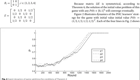
Ri=
1 0 0 1
,i∈ {1, 2, 3, 4}
E=
⎡ ⎢ ⎢ ⎣
0 1/2 0 1/2 1/2 0 1/2 0
0 1/2 0 1/2 1/2 0 1/2 0
⎤ ⎥ ⎥ ⎦
MetrixRi,i ∈ {1, 2, 3, 4}is the payoff matrix of agenti,
and elementeijof matrixEis the probability that playeri
selects playerjin each interaction. In this game, we have ui = 2 and ci = −1,i ∈ {1, 2, 3, 4}. Then the
uncon-strained dynamic model of this game is P˙ = UEP+C, where
UE=
⎡ ⎢ ⎢ ⎣
0 1 0 1 1 0 1 0 0 1 0 1 1 0 1 0
⎤ ⎥ ⎥
⎦,C=(−1,−1,−1,−1)T.
Because matrix UE is symmetrical, according to Theorem 4, the solution of the initial value problem of this game with anyP(0)∈[0, 1]4will converge eventually.
Figure 2 illustrates dynamics of the PHC learners’ strat-egy for the game with initial value initial value P(0) =
(1/2, 1/2, 1/2, 1/2)T. Each of the four lines in Fig. 2 shows
the strategy’s dynamic changing of each agent, respec-tively. We can see that the strategies of those agents con-verge eventually, which are consistent with the theoretical prediction.
Conclusion
In this work, we proposed a multiagent social learning framework to model the behavior of agent in biologic environment, and theoretically analyzed the dynamics of multiagent social learning framework using non-linear dynamic theories. We present some sufficient conditions about convergence or non-convergence and prove them by the theoretically analysis. It can be used to predict the convergence of the system. Experimental results show that the predictions of our dynamic model are consistent with the simulation results.
As future work, more extensive study of the dynam-ics of multiagent social learning framework with PHC learners is needed. Other worthwhile directions include to improve thePHCalgorithm, to develop more realistic multiagent social learning framework to model the realis-tic interactions among cells in biologic environments, and to achieve better convergence performance based on our theoretical findings.
Acknowledgements
We thank the reviewers’ valuable comments for improving the quality of this work.
Funding
This work has partially been sponsored by the National Science Foundation of China (No. 61572349,61572355).
Availability of data and materials
All data generated or analysed during this study are included in this published article.
About this supplement
This article has been published as part of Journal of Biomedical Semantics Volume 8 Supplement 1, 2017: Selected articles from the Biological Ontologies and Knowledge bases workshop. The full contents of the supplement are available online at https://jbiomedsem.biomedcentral.com/articles/ supplements/volume-8-supplement-1.
Authors’ contributions
CZ contributed to the algorithm design and theoretical analysis. SL had a main role in the editing of the manuscript. XL and ZF contributed equally to the the quality control and document reviewing. All authors read and approved the final manuscript.
Ethics approval and consent to participate
Not applicable.
Consent for publication
Not applicable.
Competing interests
The authors declare that they have no competing interests.
Author details
1School of Computer Science and Technology, Tianjin University, Peiyang Park
Campus: No.135 Yaguan Road, Haihe Education Park, 300350 Tianjin, China.
2School of Computer Computer Software, Tianjin University, Peiyang Park
Campus: No.135 Yaguan Road, Haihe Education Park, 300350 Tianjin, China.
Published: 20 September 2017
References
1. Kang S, Kahan S, Mcdermott J, Flann N, Shmulevich I. Biocellion: accelerating computer simulation of multicellular biological system models. Bioinformatics. 2014;30(21):3101–8.
2. Peng J, Bai K, Shang X, Wang G, Xue H, Jin S, Cheng L, Wang Y, Chen J. Predicting disease-related genes using integrated biomedical networks. BMC Genomics. 2017;18(1):1043.
3. Malanchi I, Santamaria-Martínez A, Susanto E, Peng H, Lehr HA, Delaloye JF, Huelsken J. Interactions between cancer stem cells and their niche govern metastatic colonization. Nature. 2012;481(7379):85–9. 4. Buehler MJ, Ballarini R. Materiomics: Multiscale Mechanics of Biological
Materials and Structures. Vienna: Springer Vienna; 2013.
5. Kaelbling LP, Littman ML, Moore AW. Reinforcement learning: A survey. J Artif Intell Res. 1996;4(1):237–85.
6. Hao J, Huang D, Cai Y, Leung H-f. The dynamics of reinforcement social learning in networked cooperative multiagent systems. Eng Appl Artif Intell. 2017;58:111–22.
7. Hao J, Leung HF, Ming Z. Multiagent reinforcement social learning toward coordination in cooperative multiagent systems. Acm Trans on Autonomous and Adaptive Systems. 2014;9(4):374–8.
8. Hao J, Leung HF. The Dynamics of Reinforcement Social Learning in Cooperative Multiagent Systems. In: Proceedings of the Twenty-Third International Joint Conference on Artificial Intelligence. Beijing: AAAI Press; 2013. p. 184–90.
9. Busoniu L, Babuska R, De Schutter B. A comprehensive survey of multiagent reinforcement learning. IEEE Trans Syst Man Cybern C. 2008;38(2):156–72.
10. Peng J, Li H, Liu Y, Juan L, Jiang Q, Wang Y, Chen J. Intego2: a web tool for measuring and visualizing gene semantic similarities using gene ontology. BMC Genomics. 2016;17(5):530.
11. Peng J, Wang T, Wang J, Wang Y, Chen J. Extending gene ontology with gene association networks. Bioinformatics. 2016;32(8):1185–94. 12. Torii M. Detecting concept mentions in biomedical text using hidden
markov model: multiple concept types at once or one at a time? J Biomed Semant. 2014;5(1):3–3.
13. Anderson ARA, Chaplain MAJ. Cheminform abstract: Continuous and discrete mathematical models of tumor-induced angiogenesis. ChemInform. 1999;30(9):857–9943.
14. Xavier JB, Martinezgarcia E, Foster KR. Social evolution of spatial patterns in bacterial biofilms: when conflict drives disorder. Am Nat. 2009;174(1): 1–12.
15. Ferrer J, Prats C, López D. Individual-based modelling: An essential tool for microbiology. J Biol Phys. 2008;34(1):19–37.
16. Jeannin-Girardon A, Ballet P, Rodin V. An Efficient Biomechanical Cell Model to Simulate Large Multi-cellular Tissue Morphogenesis: Application to Cell Sorting Simulation on GPU. In: Theory and Practice of Natural Computing: Second International Conference, TPNC 2013, Cáceres, Spain, December 3-5, 2013, Proceedings. Berlin: Springer Berlin Heidelberg; 2013. p. 96–107.
17. Matignon L, Laurent GJ, Fort-Piat NL. Independent reinforcement learners in cooperative markov games: a survey regarding coordination problems. Knowl Eng Rev. 2012;27(1):1–31.
18. Bloembergen D, Tuyls K, Hennes D, Kaisers M. Evolutionary dynamics of multi-agent learning: a survey. J Artif Intell Res. 2015;53(1):659–97. 19. Li J, Qiu M, Ming Z, Quan G, Qin X, Gu Z. Online optimization for
scheduling preemptable tasks on iaas cloud systems. J Parallel Distrib Comput. 2012;72(5):666–77.
20. Abdallah S, Lesser V. A multiagent reinforcement learning algorithm with non-linear dynamics. J Artif Intell Res. 2008;33(1):521–49.
21. Zhang C, Lesser VR. Multi-agent learning with policy prediction. In: Proceedings of the Twenty-Fourth AAAI Conference on Artificial Intelligence. Atlanta: AAAI Press; 2010.
22. Chakraborty D, Stone P. Multiagent learning in the presence of memory-bounded agents. Auton Agent Multi-Agent Syst. 2014;28(2):182–213. 23. Song S, Hao J, Liu Y, Sun J, Leung H-F, Zhang J. Improved EGT-Based
24. Bowling M, Veloso M. Multiagent learning using a variable learning rate. Artif Intell. 2002;136(2):215–50.
25. Shilnikov LP, Shilnikov AL, Turaev DV, Chua LO. Methods of Qualitative Theory in Nonlinear Dynamics. Singapore: World Scientific; 1998. 26. Singh SP, Kearns MJ, Mansour Y. Nash convergence of gradient
dynamics in general-sum games. In: Proceedings of the 16th Conference on Uncertainty in Artificial Intelligence. San Francisco: Morgan Kaufmann Publishers Inc.; 2000. p. 541–8.
27. Olshevsky V, Tyrtyshnikov EE. Matrix methods: theory, algorithms and applications: dedicated to the memory of Gene Golub. Hackensack: World Scientific; 2010. p. 604.
• We accept pre-submission inquiries
• Our selector tool helps you to find the most relevant journal
• We provide round the clock customer support
• Convenient online submission
• Thorough peer review
• Inclusion in PubMed and all major indexing services
• Maximum visibility for your research
Submit your manuscript at www.biomedcentral.com/submit