SRef-ID: 1684-9981/nhess/2004-4-513
© European Geosciences Union 2004
and Earth
System Sciences
A direction finding technique for the ULF electromagnetic source
V. V. Surkov1, O. A. Molchanov2, and M. Hayakawa3
1Moscow Engineering Physics Institute, State University, Moscow, Russia 2Institute of Physics of the Earth, Russian Academy of Sciences, Moscow, Russia 3The University of Electro-Communications, Chofu Tokyo, Japan
Received: 22 June 2004 – Revised: 15 September 2004 – Accepted: 16 September 2004 – Published: 20 September 2004 Part of Special Issue “Precursory phenomena, seismic hazard evaluation and seismo-tectonic electromagnetic effects”
Abstract. A technique of direction finding is proposed, which can be applied to the magnetic-dipole type source lo-cated in the conductive ground. To distinguish a weak ULF source signal from the natural noise a network of multicom-ponent magnetometers is supposed to be used. The data ob-tained by the ground-based stations is processed in such a way that a set of partial derivatives of the magnetic perturba-tions due to the source are found. Comparing these deriva-tives with theoretical formulae makes it possible, in princi-ple, to find the ULF source parameters such as the distance and amplitude. Averaging the data and a special procedure are proposed in order to exclude random fluctuations in the magnetic moment orientation and to avoid hydrogeological and other local factors.
1 Introduction
The problem of direction finding of the underground source as well as the problem of searching of a weak electromag-netic signal in the background of natural ionospheric and magnetospheric noise and man-made interference are of a special interest in geophysical studies. For instance, obser-vations of the weak ULF electromagnetic signals before a strong crust earthquakes with magnitudeM>6 have been re-ported by a number of authors (e.g. Fraser-Smith et al., 1990; Bernardi et al., 1991; Kopytenko et al., 1990; Molchanov et al., 1992; Hayakawa et al., 1996, 2000; Kawate et al., 1998; Singh et al., 2003; Varotsos et al, 2003a, 2003b). Whether these signals are really associated with tectonic activity and earthquake preparation process have been a subject for re-cent discussions. In this sense a crucial method in solving the above-mentioned problem could be finding the source signal location.
In order to solve this problem one comes across a number of serious difficulties and complexities. First, the character-Correspondence to: V. V. Surkov
istic wavelength (in vacuum) in the ULF frequency range is so large that an observer is always situated in the near zone, i.e. in such a case the traditional radiowave methods, such as the wave time lag measurement or miscellaneous interfer-ence schemes, are inapplicable. Second, in practice, the ULF source of interest is seemingly located under the ground, may be at higher depth. In such a case the electromagnetic signals undergo a strong dissipation and dispersion since the ULF field spreading in conductive layers of the ground is governed by the diffusion law.
In spite of this fact Kopytenko et al. (2000, 2002) and Ismaguilov et al. (2003) have proposed a special technique for searching of the underground ULF source. A network of the ground-recording stations equipped with magnetome-ters was used to detect the time lag or the phase difference between signals recorded at different points. This technique is not reliable enough since the front of signal widens due to the strong dispersion mentioned above. Besides, the typi-cal time-stypi-cale of the signals that can be related to earthquake precursor is as large as several tens minutes or hours so that the front of signals is practically absent.
The concept of another technique based on the amplitude difference measurements at different stations is the subject of present study. This technique can be applied just for the cases when the time lag and phase difference are hardly detectable.
2 Direction finding in the case of two ground-recording stations
514 V. V. Surkov et al.: A direction finding technique for the ULF electromagnetic source
z y
x O
M M
l
α1 α2
pm
z'
x'
y'
r0
Fig. 1. An illustration of equipment arrangement and the magnetic dipole location.
hundreds kilometers. Hence the mean ground parameters can be applied to study the field distribution.
In the model proposed by Surkov (1997, 1999) and Surkov et al. (2003) the effective magnetic moment results from the geomagnetic perturbations due to energization of crack for-mation in fracture zones in the vicinity of the fault. Acous-tic emission of the cracks in conductive layers of the ground excites the geomagnetic perturbations and telluric currents in such a way that the net magnetic momentpmmust be pointed oppositely to the vector of geomagnetic induction.
We cannot come close to specifying the origin of the mag-netic dipole in any detail, but we consider the case of ar-bitrary transient magnetic dipole which is immersed in the uniform half-space with constant conductivityσ. The exact solution of the problem that takes into account the boundary condition at the ground surface have been obtained by Wait and Campbell (1953). It follows from this solution that the ULF electromagnetic field spreading in conductive medium obeys the diffusion law. For example, once the source “turns on” at the momentt =0, the electromagnetic perturbations at arbitrary momenttare basically concentrated within area restricted by the radiusrd ∼ 2
√
Dt, whereD = (µ0σ )−1
denotes the coefficient of magnetic diffusion in the conduc-tor medium andµ0is the magnetic constant. Hence the
ve-locity of the perturbations front propagation can be roughly estimated asvd ∼ ˙rd ∼
√
D/t.
According to our recent study, the signals possibly asso-ciated with impending earthquakes have been detected no farther than r ∼100−200 km from the earthquake epicen-ter, as documented in many publications (e.g. see a review by Surkov (2000), and references therein, Hayakawa and Molchanov, 2002; Hayakawa and Hattori, 2004). The prop-agation time for the signals can be estimated as follows td ∼ r2/(4D) =µ0σ r2/4. Taking the above distances and
the conductivity of the upper crustσ =10−3S/m, we obtain td ∼3–12 s. The characteristic velocity of the perturbation propagation isvd ∼2/(µ0σ r) ∼8–16 km/s. Once the
dis-tance between two ground-recording stations is of the order ofl∼10 km, the lag time between the onset times is of order 1t ∼µ0σ rl/2=0.6–1.3 s.
It is usually the case that the duration of the seismogenic signals varies from several tens minutes till hours. The same period of variation,T, might be typical for the source itself. Since T td andT 1t the shape of observed signal is practically independent of the propagation timetd and the time lag 1t. This means that the electromagnetic field of the underground source can be calculated in quasi-stationary approximation. To first order in frequency the exact solution of the problem obtained by Wait and Campbell (1953) is thus transformed to the form
B= −µ0
4π∇
pm·r
r3 , (1)
which coincides with the field of magnetic dipole in the free space, that is the well-known Bio-Savart’s law. It is not wonder because in the low-frequency limit the correspond-ing skin-length tends to infinity. Note that pm in Eq. (1) should be considered as a slowly varying function of time with characteristic periodT td.
It is clear that the problem of direction finding cannot be solved in the presence of single ground-recording station and so two stations are necessary at least. The spatial scale of the ULF background noise originated from the ionosphere-magnetosphere origin is of the order of hundreds and thou-sands kilometers. Suppose this spatial scale is much greater than the characteristic length of the perturbations generated by the ULF source. The influence of background noise can then be eliminated by subtraction of the data obtained by two magnetometers located not far from each other. Let the first magnetometer be at the originO of the coordinate system and the second one is on the x-axis at the distancel. The z-axis points upwards.
In geophysical research the source of interest can be sit-uated in the vicinity of a crust fault or in an earthquake hypocenter at higher depth. If the source area is approxi-mately coincides with focal zone, its characteristic size can seemingly be as much as several tens kilometers. In this case the lumped dipole approximation is applied if only the dis-tance from the source is much greater than its characteristic size.
In this study the point magnetic dipole is assumed to be at fixed point with coordinater0 = {x0, y0, z0}to be
deter-mined. The direction of the magnetic moment vectorpmis defined by two accidental anglesα1andα2shown in Fig. 1,
so that the magnetic moment projections onto the coordinate axes,px,pyandpz, are random quantities as well.
Assuming for the moment the anglesα1andα2are
deter-minate/fixed, the magnetic field of the point moment is given by Eq. (1). If the distance from the momentr0l, one can
use the approximate formula1B ≈(l· ∇)Bfor the magne-tometer recording difference. The increment1B is
theoreti-cally expressed through partial derivatives of Eq. (1). Using the abbreviations∂i =∂/∂i, we get
∂iBj =A aijpx+bijpy+cijpz
V. V. Surkov et al.: A direction finding technique for the ULF electromagnetic source 515 wherei=x, yandj =x, y, z.
Here the following coefficients are used axx =cosβ1
3−5 cos2β1
,
axy=ayx=bxx=cosβ2
1−5 cos2β1
,
axz =cxx =cosβ3
1−5 cos2β1
,
ayy=bxy=byx =cosβ1
1−5 cos2β2
,
ayz =bxz=cxy=cyx = −5 cosβ1cosβ2cosβ3, (3)
byy=cosβ2
3−5 cos2β2
,
byz =cyy=cosβ3
1−5 cos2β2
,
cxz =cosβ1
1−5 cos2β3
,
cyz =cosβ2
1−5 cos2β3
,
A= 3µ0
4π r04 !2
.
The direction cosines, cosβ1=
x0
r0
,cosβ2=
y0
r0
,cosβ3=
z0
r0
,
that give the direction to the source are related as follows, cos2β1+cos2β2+cos2β3=1. (4)
Now we take into account the accidental character of the magnetic moment. In this consideration, the accidental alternating-sign functions in Eq. (2) should be replaced by its mean square values
D ∂iBj
2E
=Aa2ijDp2xE+b2ijDpy2E+c2ijDp2zE+2aijbij
pxpy
+2aijcijhpxpzi +2bijcijpypz. (5)
Assuming for the moment, there is an equal probability for direction of the magnetic moment vector, and then we get
p2x=Dp2yE=p2z=p2p23 . The probabilities for the projections are independent with each other in such a way thatpxpy
= hpxpzi =
pypz
=0. Since the source loca-tion is assumed to be constant, the anglesβ1,β2andβ3are
independent of time. It follows from Eqs. (3)–(5), then
(∂xBx)2=A1 5 cos4β1−2 cos2β1+1,
D ∂xBy
2E
=A1 cos2β1+cos2β2+5 cos2β1cos2β2,
(∂xBz)2=A1 cos2β1+cos2β3+5 cos2β1cos2β3,
(6)
where
A1=
1 3A
D
p2E=3Dp2E µ0 4π r04
!2 .
The sets of Eqs. (6) and (4) can be solved for direction cosines
cos2β1=51a
1 n
a1+2+(a1+2)2+5a1 1/2o
,
cos2β2=
a2 5 cos4β1−2 cos2β1+1
1+5 cos2β
1 .
(7)
l
1z
y
x
O
z
1y
1x
1O
1M
z
2y
2x
2O
2l
2p
mz
y
r
0α1
α2
x
z
'
θ M
M
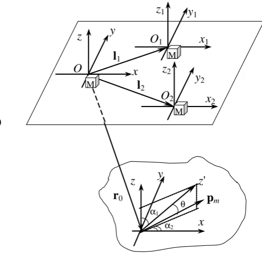
Fig. 2. A schematic drawing of the equipment arrangement and the local coordinate systems. The predominant direction for pmis
shown by z0-axis.
Here we made use of the following abbreviations
a1=1+
D ∂xBy
2E
+
(∂xBz)2
(∂xBx)2
, a2=
D ∂xBy
2E
(∂xBx)2
. (8)
The direction cosine cos2β3is derivable from Eq. (4). The
derivatives in Eq. (8) can be evaluated through the average squared differences obtained at different points.
(∂xBx)2≈l12
(1Bx)2, D
∂xBy2 E
≈ 1
l2 D
1By2 E
,
(∂xBz)2≈l12
(1Bz)2.
(9)
Herelis the distance between two three-component magne-tometers. Based on Eqs. (7)–(9) and empirical data one can find, in principle, the direction to the source.
Taking into account that the direction cosines must be smaller than unity, we obtain the limitationsa1 >5/3 and
a2<1. It is obvious, if that is not the case, the assumption on
homogeneous probability distribution for the direction ofpm is not true. In such a case the more complicated technique should be applied.
3 Direction finding in the case of three ground-recording stations
516 V. V. Surkov et al.: A direction finding technique for the ULF electromagnetic source are placed at three different points. One of them is located at
the origin of coordinate systemO, the places of the second and third magnetometers are shown by the vectorsl1andl2
in Fig. 2. Let z-axis be directed vertically upward while the x-axis points from the West to the East and the y-axis points from the South to the North. For convenience we also use the local Cartesian coordinate systems with their origins at points O1andO2. The corresponding axes,x1,y1,z1andx2,y2,z2,
are chosen to be parallel each other as shown in Fig. 2. The lumped magnetic dipolepm is characterized by the radius vectorr0 ={x0,y0,z0}and its orientation is random
(Fig. 2). Making allowance for the inequality|lk| |r0|
where k =1,2, one can use the approximate relationship 1Bk≈(lk· ∇)Bk. Hence we get
1Bi(k)=lx(k)∂xBi(k)+l (k)
y ∂yBi(k), (10)
wherelx(k)andly(k)are the projections of the vectorslk onto the coordinate axes. The set of linear equations (10) can be solved for the partial derivatives and their mean squared val-ues are
(∂xBi)2= 112
1Bi(1)l(y2)−1Bi(2)l(y1)
2
,
D ∂yBi
2E
= 1
12
1Bi(2)lx(1)−1Bi(1)l (2) x
2
,
1=lx(1)l(
2) y −l(
2) x l(
1)
y , i=x, y, z.
(11)
It should be noted that in the atmosphere only five partial derivatives ofBamong the nine are independent values since there are four connections between the derivatives following from the Maxwell’s equations∇ ×B =0 and∇ ·B =0. In our case there is the connection∂yBx = ∂xBy. It follows from this,
1Bx(1)lx(2)−1Bx(2)lx(1)=1By(2)ly(1)−1By(1)ly(2), (12) When substituting the experimental data in Eq. (12), one may expect that this equation will hold only approximately. Nev-ertheless, Eq. (12) may be used for the control of recording accuracy.
The main idea of the method proposed in the present paper is that the use of the experimental differences1Bi(k)makes it possible to evaluate the mean square of the tensor of par-tial derivativesD ∂iBj
2E
in Eq. (11). Equating these exper-imental derivatives to that given by Eqs. (3) and (5), we can estimate the mean magnetic dipole projections. On the other hand, these mean projections can be calculated theoretically. In order to estimate the averaged magnetic dipole projec-tions in Eq. (5) we suppose that there is a predominant direc-tion for the vectorpmdespite of the accidental orientation of the magnetic dipole. This direction shown in Fig. 2 by z0 -axis is defined by the constant anglesα1andα2. The
prob-ability density distribution around z0-axis is assumed to be axially symmetric so that the direction ofpmdepends solely on the polar angleθbetween the vectorpmand z0-axis. This probability distribution can be characterized by the two mean
squared projections ofpm, parallel and perpendicular to z0 -axis; that is
D p||2
E
=
D
p2cos2θ E
and Dp2⊥
E
=
D
p2sin2θ E
. (13)
The mean projections of the magnetic moment in Eq. (5) can be expressed through the mean values (Eq. 13) as follows
px2=0.5
p2⊥+passin2α1cos2α2,
D
py2E=0.5p⊥2+passin2α1sin2α2,
pz2=0.5p⊥2+pascos2α1,
pxpy
=passin2α1sinα2cosα2,
hpxpzi =passinα1cosα1cosα2,
pypz
=passinα1cosα1sinα2,
(14)
where the parameter pas=
D
p2||E−0.5Dp⊥2E
takes into account the asymmetry of the probability density distribution. In particular, if all the directions of the vector
pmhave equal probability, thenpas=0.
Substituting a set of Eq. (14) into Eq. (5), and using a set of Eq. (11), we come to a set of six equations for eight un-known parametersα1,α2,β1,β2,β3,pas,p2⊥
andA. As we have noted above, only five equations among them are in-dependent. These equations should be supplemented by the connection (Eq. 4). Nevertheless we need some additional information for solving the problem.
It is worth mentioning that in some theoretical models the crack’s acoustic emission due to rock fracture gives rise to formation of the electric currents and geomagnetic pertur-bations, whose effective magnetic moment points oppositely to the vector of local geomagnetic fieldB0 (Surkov, 1997,
1999; Surkov et al., 2003). In such a case the anglesα1and
α2 can be considered as given values since the total
mag-netic moment of whole crack ensemble is directed oppositely to the vectorB0. Note that the problem can also be solved
when the asymmetry parameter is small enough. The same technique can be developed for the ULF electric current mo-ment/dipole.
One of the challenges of the direction finding problem is to know enough the influence of the systematic errors on the results of measurements. For example, the magnetometer an-tennas cannot be quite co-directed. Besides it is possible to think about the distortions of local Earth’s electromagnetic field caused by the relief features, meteorological and hydro-geological factors, local variations of the ground conductiv-ity and etc.
In order to eliminate the influence of these and other fac-tors the data obtained in pointsO1 andO2 should be
pre-liminary corrected with respect to a reference magnetometer placed in the pointO. For example it is customary to correct these data,B1andB2, as follows
B01= ˆA1×B1, B02= ˆA2×B2,
whereAˆ1andAˆ2are the symmetric matrixes, whose
coeffi-cients are selected empirically in such a way that the quanti-tiesB0
magnetometer recording on average. In fact these matrixes slightly turn the vectors of magnetic induction in order to make the recordings compatible with each other. When cal-culating the differences1Bi(k) in Eq. (11), these corrected valuesB01andB02should be used.
4 Conclusions
This promising technique based on evaluation of the partial derivatives of the magnetic perturbations makes it pos-sible, in principle, to find both the location of the ULF magneto-dipole source and the direction cosines of the mean moment vector. The technique can be applied irrespective of the fact that either the remote source is situated in the ground, in the atmosphere or the ionosphere. In addition, this technique is valid when the signals from underground ULF source undergo strong dissipation and dispersion in conductive rock that makes difficulties in recording of time lag and phase difference of the signals. From this viewpoint, the analyses of amplitudes and spatial derivatives of the magnetic perturbations, seems, to be more perspective. There are two limitations of the technique, first, a spatial scale of natural noise variation should be much greater than both characteristic length of the ULF signal variation and distances between magnetometers, and second, the charac-teristic source size must be small compared to distance from the source. As both conditions are satisfied, the technique allows us to discriminate a weak useful ULF signal from background noise with confidence. This information can be extremely useful for interpretation of experimental data and for understanding of the origin the ULF signals and, in particular, for finding the electromagnetic signals possibly related to impending earthquakes.
Edited by: P. F. Biagi Reviewed by: two referees
References
Bernardi, A., Fraser-Smith, A. C., McGill, P. R., and Villard, Jr. O. G.: ULF magnetic field measurements near the epicenter of the Ms 7.1 Loma Prieta earthquake, Phys. Earth Planet. Inter., 68,
45–63, 1991.
Fraser-Smith, A. C., Bernardi, A., McGill, P. R., Ladd, M. E., Hel-liwell, R. A., and Villard, O. G. Jr.: Low-frequency magnetic field measurements near the epicenter of theMs7.1 Loma Prieta
earthquake, Geophys. Res. Lett., 17, 1465–1468, 1990. Hayakawa, M., Kawate, R., Molchanov, O. A., and Yumoto, K.:
Results of ULF magnetic field measurements during the Guam earthquake of 8 August 1993, Geophys. Res. Lett., 23, 241–244, 1996.
Hayakawa, M., Itoh, T., Hattori, K., and Yumoto, K.: ULF electro-magnetic precursors for an earthquake at Biak, Indonesia on 17 February 1996, Geophys. Res. Lett., 27, 1531–1534, 2000. Hayakawa, M. and Molchanov, O. A., editors: “Seismo
Elec-tromagnetics: Lithosphere-Atmosphere-Ionosphere Coupling”, TERRAPUB, 477 p., Tokyo, 2002.
Hayakawa, M. and Hattori, K.: ULF electromagnetics emissions associated with earthquakes: Review, Trans. Fundamentals and Materials, Special Issue on Electromagnetic Theory and Its Ap-plication Dec., in press, 2004.
Ismaguilov, V. S., Kopytenko, Yu. A., Hattori, K., and Hayakawa, M.: Variations of phase velocity and gradient of ULF geomag-netic disturbances connected with the Izu strong earthquakes, Nat. Haz. Earth Sys. Sci., 3, 211–215, 2003,
SRef-ID: 1684-9981/nhess/2003-3-211.
Kawate, R., Molchanov, O. A., and Hayakawa, M.: Ultra-low-frequency magnetic fields during the Guam earthquake of 8 Au-gust 1993 and their interpretation, Phys. Earth Planet. Inter., 105, 229–238, 1998.
Kopytenko, Yu. A., Matiashvili, T. G., Voronov, P. M., Kopytenko, E. A., and Molchanov, O. A.: Detection of ULF emissions con-nected with the Spitak earthquake and its aftershock activity, based on geomagnetic pulsation data at Dusheti and Vardzia ob-servations, Preprint of IZMIRAN, 1990 (in Russian).
Kopytenko, Yu. A., Ismaguilov, V. S., Kopytenko, E. A., Voronov, P. M., and Zaitsev, D. B.: Magnetic location of geomagnetic dis-turbance sources, DAN, series Geophysics, 371, 685–687, 2000. Kopytenko, Yu. A., Ismaguilov, V. S., Molchanov, O. A., Kopy-tenko, E. A., Voronov, P. M., Hattori, K., Hayakawa, M., and Zaitsev, D. B.: Investigation of ULF magnetic disturbances in Japan during seismic active period, J. Atm. Electr., 22, 207–215, 2002.
Molchanov, O. A., Kopytenko, Yu. A., Voronov, P. M., Kopytenko, E. A., Matiashvili, T. G., Fraser-Smith, A. C., and Bernardi, A.: Results of ULF magnetic field measurements near the epicen-ters of the Spitak (Ms =6.9) and Loma Prieta (Ms =7.1)
earth-quakes: comparative analysis, Geophys. Res. Lett., 19, 1495– 1498, 1992.
Singh, R. P., Singh, B., Mishra, P. K., and Hayakawa, M.: On the lithosphere-atmosphere coupling of seismo-electromagnetic sig-nals, Radio Sci., 38, 1065–1074, 2003.
Surkov, V. V.: The nature of electromagnetic forerunners of earth-quakes, Transactions (Doklady) of the Russian Academy of Sci-ences. Earth Science Sections, 355, 945-947, 1997.
Surkov, V. V.: ULF electromagnetic perturbations resulting from the fracture and dilatancy in the earthquake preparation zone, in “At-mospheric and Ionospheric Phenomena Associated with Earth-quakes”, edited by Hayakawa, M., TERRAPUB, Tokyo, 357– 370, 1999.
Surkov, V. V.: Electromagnetic effects caused by earthquakes and explosions. MEPhI press, Moscow, 2000, 448 pp. (in Russian). Surkov, V. V., Molchanov, O. A., and Hayakawa, M.:
Pre-earthquake ULF electromagnetic perturbations as a result of in-ductive seismomagnetic phenomena during microfracturing, J. Atmos. Solar-Terr. Phys., 65, 31–46, 2003.
Varotsos, P. A., Sarlis N. V., and Skordas, E. S.: Long-range corre-lations in the electric signals that precede rupture: Further inves-tigations, Phys. Rev., E67, 021109, 2003.
Varotsos, P. A., Sarlis N. V., and Skordas, E. S.: Attempt to distin-guish electric signals of a dichotomous nature, Phys. Rev., E68, 031106, 2003.