Accelerated estimation and permutation inference for ACE modeling

R E S E A R C H A R T I C L E

Accelerated estimation and permutation inference for

ACE modeling

Xu Chen

| Elia Formisano

| Gabriëlla A. M. Blokland

|

Lachlan T. Strike

| Katie L. McMahon

| Greig I. de Zubicaray

|

Paul M. Thompson

| Margaret J. Wright

| Anderson M. Winkler

|

Tian Ge

| Thomas E. Nichols

1

Department of Statistics, University of Warwick, Coventry, UK

2

Department of Cognitive Neuroscience, Faculty of Psychology and Neuroscience, Maastricht University, Maastricht, the Netherlands

3

Maastricht Centre for Systems Biology (MaCSBio), Maastricht University, Maastricht, the Netherlands

4

Department of Biomedical Data Sciences, Leiden University Medical Center, Leiden, the Netherlands

5

Psychiatric and Neurodevelopmental Genetics Unit, Center for Genomic Medicine, Massachusetts General Hospital, Boston, Massachusetts

6

Stanley Center for Psychiatric Research, Broad Institute of MIT and Harvard, Cambridge, Massachusetts

7

Department of Psychiatry, Massachusetts General Hospital, Harvard Medical School, Boston, Massachusetts

8

Queensland Brain Institute, University of Queensland, Brisbane, Queensland, Australia

9

Centre for Advanced Imaging, University of Queensland, Brisbane, Queensland, Australia

10

Faculty of Health and Institute of Health and Biomedical Innovation, Queensland University of Technology, Brisbane, Queensland, Australia

11

Imaging Genetics Center, University of Southern California, Los Angeles, California

12

Emotion and Development Branch, National Institute of Mental Health, National Institutes of Health, Bethesda, Maryland

13

Department of Psychiatry, Yale University School of Medicine, New Haven, Connecticut

14

Athinoula A. Martinos Center for Biomedical Imaging, Massachusetts General Hospital, Charlestown, Massachusetts

15

Oxford Big Data Institute, Li Ka Shing Centre for Health Information and Discovery, Nuffield Department of Population Health, University of Oxford, Oxford, UK

Correspondence

Xu Chen, Department of Biomedical Data Sciences, Leiden University Medical Center, Leiden, the Netherlands.

Email: [email protected]

Funding information

Australian Research Council, Grant/Award Numbers: A7960034, A79801419, A79906588, DP0212016; Eunice Kennedy Shriver National Institute of Child Health and Human Development, Grant/Award Number: RO1 HD050735; National Health and Medical Research Council, Grant/Award Number: 496682; National Institutes of Health, Grant/ Award Number: K99AG054573; Stichting voor de Technische Wetenschappen, Grant/Award Number: 12724

Abstract

There are a wealth of tools for fitting linear models at each location in the brain in

neu-roimaging analysis, and a wealth of genetic tools for estimating heritability for a small

number of phenotypes. But there remains a need for computationally efficient

neuro-imaging genetic tools that can conduct analyses at the brain-wide scale. Here we

pre-sent a simple method for heritability estimation on twins that replaces a variance

component model-which requires iterative optimisation-with a (noniterative) linear

regression model, by transforming data to squared twin-pair differences. We

demon-strate that the method has comparable bias, mean squared error, false positive risk, and

power to best practice maximum-likelihood-based methods, while requiring a small

fraction of the computation time. Combined with permutation, we call this approach

“

Accelerated Permutation Inference for the ACE Model (APACE)

”

where ACE refers to

the additive genetic (A) effects, and common (C), and unique (E) environmental

influ-ences on the trait. We show how the use of spatial statistics like cluster size can

DOI: 10.1002/hbm.24611

This is an open access article under the terms of the Creative Commons Attribution License, which permits use, distribution and reproduction in any medium, provided the original work is properly cited.

© 2019 The Authors.Human Brain Mappingpublished by Wiley Periodicals, Inc.

dramatically improve power, and illustrate the method on a heritability analysis of an

fMRI working memory dataset.

K E Y W O R D S

ACE model, heritability inference, permutation test, twin studies

1

|

I N T R O D U C T I O N

There continues to be growing interest in the joint study of imaging

phenotypes and genetic data (genotypes; Glahn, Thompson, &

Blangero, 2007). Imaging genetics is a multidisciplinary research area

investigating the genetic influences on brain structure and function

using both imaging and genetic information. A phenotype is an

observ-able characteristic that results from the interaction of genetic

inheri-tance and environmental conditions. To quantify the degree of the

genetic effects on a phenotype, heritability is defined as the proportion

of phenotypic variation that is due to genetic factors, where the genetic

variability can be attributed to a particular gene or the aggregate of

multiple genes. Several studies have examined the heritability of

psychi-atric disorders, and many of them suggest that most psychipsychi-atric

disor-ders are moderately to highly heritable, with an estimated heritability of

0.83 for schizophrenia (Cannon, Kaprio, Lönnqvist, Huttunen, &

Koskenvuo, 1998) and 0.85 for bipolar affective disorder (McGuffin

et al., 2003). There also exists a large number of neuroimaging studies

investigating the heritability of neuroanatomical phenotypes and brain

functions and reporting considerable heritability (see for example, Ge

et al., 2015, 2016; Ge, Holmes, Buckner, Smoller, & Sabuncu, 2017;

Glahn et al., 2010; Thompson, Ge, Glahn, Jahanshad, & Nichols, 2013).

Recently, the development of genomic technologies has allowed

direct heritability analysis from unrelated individuals using

genome-wide genetic data (Ge, Chen, Neale, Sabuncu, & Smoller, 2017; Yang

et al., 2010; Yang, Lee, Goddard, & Visscher, 2011). Without genetic

data, heritability can be estimated by studying individuals with varying

degrees of genetic relatedness. Classic twin studies are often employed

to estimate the level of genetic and environmental variations in traits.

The method of moments and the maximum likelihood approach are

most commonly used methods to estimating heritability. Falconer's

for-mula provides a simple point estimator for heritability based on moment

matching (Falconer & Mackay, 1996). The best practice,

likelihood-based method uses the variance component model, which

parameter-izes different degrees of covariance expected with varying relatedness

between subjects; the variance parameters are estimated by applying

the maximum likelihood criterion (Neale & Cardon, 1992).

While the first neuroimaging studies measuring heritability used

Falconer's method (e.g., Wright, Sham, Murray, Weinberger, &

Bullmore, 2002), the likelihood-based approach is now routine, with

variance components or structural equation modeling (SEM) methods

applied one voxel at a time. However, such methods cannot exploit

the spatial nature of the data, nor can they provide accurate

infer-ences corrected for family-wise error rate over the brain. Although a

simple Bonferroni correction offers the control of family-wise error

rate, it is typically quite conservative for smooth images. When

feasi-ble, permutation inference offers an exact control of false positive risk

and allows for specialized spatial statistics, such as inference by

clus-ter size, which delivers family-wise error rate corrections while

implic-itly accounting for spatial dependence. However, most commonly

used software tools for heritability estimation using twin data at

pre-sent are too slow and unreliable to allow permutation.

In this article, we propose a linear regression-based method that is

new to the neuroimaging community, based on the method of Grimes

and Harvey (1980) and closely related to the Haseman–Elston

regres-sion for genetic linkage studies (Ge et al., 2018; Haseman & Elston,

1972). It allows voxel-wise heritability estimation with an approximate

but remarkably fast and accurate performance. Using detailed Monte

Carlo evaluations, we demonstrate that this method is valid with

con-trolled false positive risk, and its statistical power is comparable to

existing methods. With the speed advantage, this newly proposed

method makes permutation inference more feasible and applicable.

Here we also present for the first time our permutation approach in

detail, which is developed for both voxel- and cluster-wise inferences,

with an application to a real fMRI blood oxygen level dependent

(BOLD) dataset. Aside from fMRI data, this approach can also be

applied to any other type of neuroimaging data.

2

|

T H E O R Y A N D M E T H O D S

Heritability can be interpreted as the proportion of phenotypic

vari-ance explained by a single genetic marker (Filippini et al., 2008) or any

subset of genes/markers of the genome (Stein et al., 2010). To

quan-tify heritability, the total phenotypic variance (σ2

P) can be partitioned

into genetic (σ2

G) and environmental (σ2E) components (Falconer &

Mac-kay, 1996) in a linear manner:

σ2

P=σ2G+σ2E:

The heritability in the broad sense (H2_{) measures the overall}

genetic influence on a trait, defined by

H2=σ

2 G σ2 P

,

where the genetic variationσ2

Gsummarizes the additive and

nonaddi-tive genetic contributions. The addinonaddi-tive genetic effect arises from the

contributions at different gene loci, while the nonadditive genetic

effect refers to, for example, dominance or the interactive influence

among alleles within or between gene loci (e.g., epistasis). The additive

genetic variation is generally of more interest since it is the summed

effects of a particular allele or alleles at a given locus or at multiple

trait-related loci. Thus, the narrow-sense heritability is defined as the

proportion of phenotypic variation accounted for by the additive

genetic effect (σ2

A) with an expression of

h2=σ

2 A σ2 P

,

which is more commonly used and is usually just called“heritability”.

We now detail the models employed to assess heritability using

twin data.

2.1

|

The model

2.1.1

|

Twin studies and ACE modeling

Normally twins are categorized as identical or monozygotic (MZ) and

fra-ternal or dizygotic (DZ) twins. MZ twins have identical genotypes and DZ

twins share, on average, 50% of their gene variants, which leads to the

assumption of differential levels of sharing of additive genetic effects.

Even in the absence of genetic influences on a phenotype, it is likely that

twins are phenotypically more similar than unrelated individuals since

they have been raised in the same family environment. This gives rise to

the common environmental factor, which contributes to the covariance

within twin pairs regardless of MZ or DZ type. Finally, there is an

inde-pendent unique error, corresponding to the usual indeinde-pendent and

iden-tically distributed (i.i.d.) noise corrupting the measurements plus actual

unique environmental influences, for example, trauma and illness. The

phenotypic variance (_σ2

P) within the population is assumed to be the

same and can be divided into additive genetic (A), common

environ-mental (C), and unique environmental (E) components, written as

σ2

P=A+C+E:

The so-called ACE modeling in twin studies is based on this variance

decomposition (Lee et al., 2010). Narrow-sense heritability is denoted by

h2₌ A

A+C+E, ð1Þ

and similarly, the contribution of common environmental factor can

be defined as

c2₌ C

A+C+E, ð2Þ

which describes the relative variance attributable to common

mental causes. The estimation of heritability and common

environ-mental variance constitutes the analysis of variance components.

2.1.2

|

Notation

In this section, we will outline the notation used in this article. Assume

the experiment consists ofn participants, includingnMZMZ twins

(nMZ/2 pairs),nDZDZ twins (nDZ/2 pairs), andnSsingletons (unrelated

subjects and denoted by S), such thatn=nMZ+nDZ+nS. For each

(brain) image, withV voxels per subject, Yi,vdenotes the data from

subjectiand voxelv(v= 1,_…,V). For voxelv, the data from all

sub-jects can be written as a column vectorYv.

Some types of brain imaging data are directly measured, for example,

grey matter density, producing one image per subject. However, fMRI

requires hundreds of scans per subject to estimate blood flow change. A

within-subject model is often fitted to the imaging data for each subject,

producing an image of BOLD effect magnitude for each subject

(Frackowiak et al., 2004). Since the same form of model is fit at each

voxel, going forward we suppress the voxel indexv.Thus, the general

linear model (GLM) in a matrix form for each voxel can be constructed as

Y=Xβ+ϵ, ð3Þ

whereXis ann×pdesign matrix includingp−1 covariates, andϵis

the error vector, assumed to be normally distributed, written as_ϵ~_N

(0,V); the covariance matrixV is defined below. Typical covariates

include age, sex, or other between-subject effects.

To simplify the description of variance/covariance decomposition,

we introduce a subject type indicator functionT: {1,_…,n}!{MZ, DZ,

S}. The function Tð Þ associates subject index i to subject type:

T ið Þ 2fMZ, DZ, Sgfori= 1,_…,n; that is,T ið Þ= MZ when subjectiis an

MZ twin,T ið Þ= DZ when subjectiis a DZ twin, andT ið Þ= S when

sub-jectiis a singleton. We now consider different possible covariance

structures for pairs of subjects (i,j). To identify twins, letj(i) be the

index of the twin pair of subjecti.The MZ twin covariance can then

be written, foriwithT ið Þ=T j iðð ÞÞ= MZ, as

CovMZ =Cov Yi

Yj ið Þ

!

= A+C+E A+C

A+C A+C+E

: ð4Þ

The DZ twin covariance, foriwithT ið Þ=T j iðð ÞÞ= DZ, is

CovDZ =_Cov Yi

Yj ið Þ

!

= A+C+E A=2 +C

A₌2 +C A+C+E

: ð5Þ

For subject pairs involving one or more singletons from different

families without twins, (i, j) with T ið Þ= S or T jð Þ= S, or pairs of

unrelated twins, (i,j) withj6¼j(i), we have unrelated covariance of

CovUN =_Cov Yi

Yj

= A+C+E 0

0 A+C+E

: ð6Þ

To facilitate a general implementation, we re-write the pair-wise

covariance matrices for MZ twins (4), DZ twins (5) and unrelated

sub-jects (6) as the linear combinations of some known matrices,

CovMZ = A+C+E A+C

A+C A+C+E

=A 1 1

1 1

+C 1 1

1 1

+E 1 0

0 1

,

ð7Þ

CovDZ = A+C+E A=2 +C

A₌2 +C A+C+E

=A 1 1=2

1₌2 1

+C 1 1

1 1

+E 1 0

0 1

,

ð8Þ

CovUN = A+C+E 0

0 A+C+E

=A 1 0

0 1

+C 1 0

0 1

+E 1 0

0 1

,

ð9Þ

where variance components are extracted as the coefficients. If we

denote the vector of variance componentsA,C,Eby_ρ= (A,C,E)0, a

concise notation of the error variance-covariance matrixVis

V=X

3

r= 1 ρrQr,

whereQr(r= 1, 2, 3) is constructed with the use of between-subject

covariances (7), (8), and (9), corresponding to the arrangement of MZ,

DZ and singletons in the data vector. The full likelihood and restricted

likelihood (ReML) that accounts for nuisance regressors can be found

in (Harville, 1977).

2.2

|

Voxel-wise heritability estimation

For each voxel, we fit the GLM model to the voxel-wise data from

twins and singletons, then estimate the model parameters—variance

components, and finally obtain the estimate of heritability. We will

first describe our proposed method in detail, and then briefly review

other methods/tools that are widely used for heritability estimation.

2.2.1

|

Linear regression with squared differences

In the 1980s, a simple linear regression method for variance component

estimation using squared differences (SqD_’s) of each subject pair was

proposed by Grimes and Harvey (1980). For a sample ofnsubjects,

there are (n2−n)/2 distinct SqD’s. Note that the expectation of a SqD

depends on the covariance, that is,EhðA−BÞ2i=VarðA−BÞ=Varð ÞA + Varð ÞB −2CovðA,BÞfor random variablesAandBwithE½ A=E½ B. This allows SqD's to be related to variance parameters in a linear fashion,

in particular construction of a linear regression where coefficients

cor-respond to the variance componentsA,C,E(Grimes & Harvey, 1980;

Lindquist, Spicer, Asllani, & Wager, 2012). Grimes and Harvey (1980)

used ordinary least squares (OLS), which can produce negative

vari-ance component estimates that they simply neglected.

To deal with the non-negativity problem, Lawson and Hanson (1987)

proposed a now ubiquitous non-negative least squares (NNLS) algorithm.

The foundation of this algorithm is the Karush–Kuhn–Tucker (KKT)

con-ditions (Karush, 1939; Kuhn & Tucker, 1951), which were first proposed

for more complex nonlinear programming problems. In our case with the

linearity assumption, the KKT conditions can be simplified to accelerate

the computation. Although other methods had been proposed to solve

this non-negativity problem for large and sparse matrix settings, Luo and

Duraiswami (2011) suggested that NNLS still maintained its superiority

when small or moderate dense matrices were handled.

While Grimes and Harvey's method specifies a linear regression with

the use of (n2−n)/2 different observations of SqD’s, our modification of

this method simplifies the computation such that only (nMZ+nDZ)/2

observations are utilized in computing SqD_’s. Thus, the integration of the

construction of the linear regression model with SqD_’s and estimating

variance-covariance parameters using NNLS with computational

modifi-cation yields a novel and fast NNLS regression approach for unknown

variance component estimation, entitled“Accelerated Permutation

Infer-ence for the ACE model (APACE)”. The method of linear regression

model construction with SqD_’s vary depending on whether

subject-specific covariates are included in the GLM model or not.

One sample model

Consider the case when the original GLM (3) is a simple linear

regres-sion model with an intercept only:

Y=1_β0+ϵ, ð10Þ

where1is an all-ones vector andβ0denotes the population mean. By the

extension of the covariance matrices (4), (5), and (6) and the basic

proper-ties of the variance operator, for MZ twin pairs (i,j(i)),T ið Þ= MZ, we have

EYi−Yj ið Þ2

h i

=_Var_ϵi−ϵj ið Þ= 2E, ð11Þ

for DZ twin pairs (i,j(i)),T ið Þ= DZ, we have

EYi−Yj ið Þ2

h i

=Varϵi−ϵj ið Þ=A+ 2E, ð12Þ

and for unrelated pairs of subjects (i,j),

E Yi−Yj2

h i

=Varϵi−ϵj= 2A+ 2C+ 2E: ð13Þ

The relationships (11), (12), and (13) describe the expected values

for all these (n2

−n)/2 SqD_’s and specify the mean structure of a

lin-ear regression model:

E

Y1−Yjð Þ1

2

...

YnMZ=2 + 1−Yj nðMZ=2 + 1Þ

2

...

Yi−Yj

2 ... 0 B B B B B B B B B B B B B @ 1 C C C C C C C C C C C C C A 2 6 6 6 6 6 6 6 6 6 6 6 6 6 4 3 7 7 7 7 7 7 7 7 7 7 7 7 7 5 = 0 0 2

...

1 0 2

...

2 2 2

... 0 B B B B B B B B B B @ 1 C C C C C C C C C C A A C E 0 B @ 1 C A,

where the firstnMZ/2 rows are the SqD’s of MZ twins, the nextnDZ/2

rows are for the DZ twins, and the remaining (n2

−nDZ/2 rows are for the remaining unrelated subject pairings. We denote this as

E½ D =Z_ρ, ð14Þ

where,Dis an (n2−n)/2×1 SqD vector of observations,Zis an (n2−n)/

2_×3 design matrix, and_ρis the unknown variance parameter vector.

Multiple linear regression

Now suppose that the GLM (3) is a multiple regression model

con-taining an regression intercept and multiple covariates, expressed as

Y=1_β0+X1β1+…+Xp−1βp−1+ϵ, ð15Þ

where then-vectorsX1,_…,Xp−1are regressors, each associated with

one of thep−1 covariates, andβ1,…,βp−1are the corresponding

regression coefficients. The parameters_β= (_β0,_…,_βp−1)

0

are not of

interest and we treat them as nuisance parameters in variance

compo-nent analysis. If we estimate _β using OLS with an expression of

^

βOLS=ðX0XÞ−1X0Y, whereX= (1,X1,…,Xp−1) is the complete design

matrix, the resulting OLS residuals are

e=Y₋X_βOLS^ = I₋X Xð 0XÞ−1 X0

Y_: ð16Þ

Denote the residual projection matrix byR=I₋X(X0X)−1_X0

, and

the OLS residual vectore=RY follows a normal distribution with

meanE½ e=0and varianceCov(e) =RVR, that is,e~N(0,RVR), where

the projection matrixRprojects the unobservable error vector_ϵto its

estimateethat is orthogonal to the space spanned by the columns of

the design matrixX. When the sample sizenis large enough, the error

vector _ϵ can be well approximated by the residual vector e. We

assume that the correlation induced by removing covariates and mean

centering is negligible when compared with variance components,

that is,RVR≈V, which is a reasonable assumption for sufficientn.

Here the variance components are derived in terms of

nuisance-free errors:

Eei−ej ið Þ2

h i

=Varei−ej ið Þ≈2E

for MZ twin pairs,

Eei−ej ið Þ2

h i

=Varei−ej ið Þ≈A+ 2E

for DZ twin pairs, and

E ei−ej

2

h i

=_Var ei−ej

≈2A+ 2C+ 2E_:

for the remaining unrelated subject pairs. Therefore, the derived linear

regression model with SqD’s can be analogously denoted as

E½ D≈Zρ: ð17Þ

Computational simplification For largen, the (n2

−n)/2 rows of the SqD data and design matrix is

unwieldy. Hence we modify how we compute estimatesρ^=ðZ0ZÞ−1

Z0D. First,Z0Zis directly found as

Z0Z=

nDZ=2 + 4notw 4notw nDZ+ 4notw

4notw 4notw 4notw

nDZ+ 4notw 4notw 2n2−n

0 B @ 1 C A,

wherenotw= (n

2

−n)/2−nMZ/2−nDZ/2. Next, observe that

Z0D=

PðnMZ+nDZÞ=2 l=nMZ=2 + 1 Dl+ 2

Pðn2_−nÞ₌₂ l=ðnMZ+nDZÞ=2 + 1Dl

2Pn

2_−n

ð Þ=2 l=ðnMZ+nDZÞ=2 + 1Dl

2Pn

2_−n

ð Þ=2 l= 1 Dl 0 B B B B @ 1 C C C C A =

2SSD₋2SSDMZ−SSDDZ

2SSD₋2SSDMZ−2SSDDZ

2SSD 0 B @ 1 C A,

where, Dlis thel

th

element ofD, SSD =Pn

2_−n

ð Þ=2

l= 1 Dlis the sum of all

squared differences, SSDMZis the sum ofnMZ/2 squared differences

for MZ, and SSDDZis the sum ofnDZ/2 squared differences for DZ. A

fundamental result (see Appendix A) shows that SSD is just a multiple

of the sample variance:

SSD =n2−ns2ð ÞY,

where s2_{ð ÞY =}Pn

i Yi−Y

2

=ðn−1Þ. With the nuisance variables, we

approximate this sum with the residual variance from the GLM (3),

that is,

SSD≈n2_−nσ^2_,

where_σ^2_=e0_{e=ðn−pÞis the unbiased estimator for the phenotypic}

varianceσ2. With simulations, we verified that estimating SSD with

this residual variance had a negligible impact on parameter estimates.

Non-negative least squares

Our APACE method proceeds by applying the NNLS algorithm to the

linear regression model with SqD_’s (10) or (15) for unknown variance

component estimation; precisely, we seek

min_ρfð Þ_ρ s_:t_:ρ≥0,

wheref(ρ) =kZρ−Dk2/2 is the objective function to be minimized.

KKT conditions provide the necessary conditions for this optimization

problem: Ifρ* is the local minimizer off(ρ) satisfying the inequality

constraint_ρ≥0, then the following conditions hold:

rf_ρ* 0_ρ*= 0,rf _ρ* _≥0,_ρ*_≥0,

where, the gradient vector isrf(_ρ) =Z0(Z_ρ−D) (Karush, 1939; Kuhn &

Tucker, 1951). AsZ0(Zρ−D) =0corresponds to the least squares

nor-mal equations, for anyZ,D, and_ρfound by OLS, the first two

condi-tions are trivially satisfied, and hence, only the third condition needs

estimate_ρand checking for negative elements. If a negative element

is found, it is set to zero, effectively dropping that column from theZ,

and OLS is re-fit.

Algorithm simplification

The NNLS algorithm can be further modified and simplified for the

computation in ACE modeling since there are only three parameters

A,C,Ein total. There are only a total of 23−1 = 7 possible models

that can arise under NNLS, but we require the unique environmental

factorEto always be present due to the unavoidable measurement

error or noise. Thus we only need to consider four possible models E,

AE, CE, and ACE withρE= (0, 0,E)

0

, ρAE= (A, 0,E) 0

, ρCE= (0,C,E) 0

and_ρACE= (A,C,E) 0

representing the vectors of unknown parameters,

respectively.

Since the space of possible models is so small, we can enumerate

and evaluate these four models. We first fit the full ACE model, and if

all theA,C,Eparameters are non-negative, this estimateρACE^ is used;

otherwise, the remaining estimatesρE^,ρAE^ , andρCE^ corresponding to

the three restricted models are computed. Among the optional models

with valid estimates (i.e., all non-negative), the best fitting model is

selected; as valid AE and CE models will always explain more

variabil-ity than an E model, these are next selected when available. If both

AE and CE models have valid estimates, we have two methods to

assess the model fit. The model with the smallest residual sum of

squares, that is,ðD−Zρ^Þ0ðD−Zρ^Þ, can be selected, which is our default APACE setting. Alternatively, we can return to the original GLM

model (3) and select the model with the higher ReML log-likelihood

for APACE-computed_ρAE^ and_ρCE^ . This process to choose between

the two models is equivalent to using a model selection method based

on Akaike's information criterion or Bayesian information criterion.

Likelihood ratio test

Tests on parameter estimates are performed as usual, with a likelihood

ratio test (LRT) comparing the fitted model (alternative model) H1:A> 0

to the null model H0:A= 0, that is, the full ACE model is compared to

the nested CE model, or AE to E. The LRT statistic is defined as

T=−2×½ℓðρ0^jYÞ−ℓðρ1^jYÞ,

where,ρ0^ andρ1^ are parameter estimates derived from the null and

alternative models, respectively, and_ℓð_ρ^jYÞis the ReML log-likelihood

given observationsY. Under the assumption of normality, the

likeli-hood function can be analytically computed (see for example, Harville,

1977). Wilks' theorem states that under certain regularity conditions,

the null distribution of the LRT statistic for comparing nested models

(e.g., CE vs. ACE) converges to a chi-squared distribution asn!∞

(Wilks, 1938). In particular,Tis usually regarded to asymptotically

fol-low a chi-squared distribution with 1 degree of freedom, that is,_χ2

1,

based on Wilks' theorem. However, the null value of the variance

parameterAlies on the boundary of the parameter space and thus the

asymptotic sampling distribution of this LRT statistic, under H0, is a

half-half mixture of chi-squared distributions, that is, _χ2_{0=2 +χ}2_1=2,

instead of a commonly used standard chi-square distribution, that is, χ2

1(Dominicus, Skrondal, Gjessing, Pedersen, & Palmgren, 2006; Self &

Liang, 1987; Zhang & Lin, 2008).

Given the asymptotic null distribution of the LRT statistic, the

theo-reticalp-value can be easily calculated. Obtaining ap-value less than a

given significance level α, which is typically a small number

(e.g.,α= 0.05), suggests that there is significant evidence against the null

hypothesis and the null hypothesis should be rejected at levelα.We

note that when data is non-Gaussian, the LRT computed under the

nor-mality assumption can be inaccurate and the use of Wilk's theorem in

approximating its null distribution might lead to invalid results, which will

be investigated in our simulation studies. We therefore compute both

the asymptotic theoreticalp-value and the permutation-basedp-value

based on the empirical distribution of the LRT statistic (see below).

2.2.2

|

Existing methods

Several approaches have been proposed for the analysis of

heritabil-ity, and we briefly introduce these existing approaches in this section.

Falconer's method

The heritability method due to Falconer and Mackay (1996) is based

on moment matching of intraclass correlation coefficients between

MZ twins (rMZ) and DZ twins (rDZ):

E½rMZ=

A+C A+C+E,

E½rDZ=

A=2 +C A+C+E:

8 > > < > > :

Solving for narrow-sense heritability (2), these equations give

Fal-coner's heritability estimator:

^

h2_F= max 0, 2ð ðrMZ−rDZÞÞ:

This method has been widely used and is the simplest way to

esti-mate heritability (Falconer & Mackay, 1996). However, methods of

moments estimators can perform poorly relative to optimal maximum

likelihood estimators (Nichols, Friston, Roiser, & Viding, 2009). We

consider this in a small set of simulations, described below.

The null hypothesis of zero heritability can be tested by comparing

the MZ and DZ correlation coefficients after Fisher's

variance-stabilising transformation. For MZ, Fisher's transformation is

zMZ=

1

2log

1 +rMZ

1−rMZ

,

which is approximately normally distributed with mean

E½zMZ=

1

2log

1 +ρMZ

1_−ρMZ

VarðzMZÞ=

1

n_MZ=2₋3,

where_ρMZis the true population correlation coefficient; likewise for

zDZ. To test for the equality ofrMZandrDZ, that is, zero heritability,

we can use the test statistic

TF=

zMZ−zDZ

ffiffiffiffiffiffiffiffiffiffiffiffiffiffiffiffiffiffiffiffiffiffiffiffiffiffiffiffiffiffiffiffiffi

1 nMZ=2−3+

1 nDZ=2−3

q 1 _h2

F> 0

f g,

where1{}is the indicator function. Without the positivity constrain,

this test statistic would be asymptotically distributed as a standard

normal distribution under H0(Sakaori, 2002). Considering the

positiv-ity constraint, we consider the null distribution to be a half-half

mix-ture of a point mass at zero (a.k.a._χ2

0) and a half normal distribution.

Bayesian ReML

Statistical parametric mapping (SPM) software (http://www.fil.ion.ucl.

ac.uk/spm) provides a general framework for variance component

model estimation in a Bayesian setting, and, as a special case, can

implement the ACE model. Based on preliminary studies (Nichols

et al., 2009), we show that this Bayesian approach produces

heritabil-ity estimates with lower bias and variance than Falconer's method.

SPM's Bayesian ReML uses a log Gaussian prior on variance

parame-ters, ensuring non-negative variance parameter estimates. We set the

prior mean and variance of the log variance parameters to be

hE = logðVar Yð ÞÞ−1 andhC = exp(8) to produce uninformative priors.

We considered perturbations of these settings but simulations found

that these priors were best in terms of estimation accuracy and power

(not shown). SPM uses the expectation-maximization (EM) algorithm

to iteratively search for the maximum a posteriori estimates of the

parameters in the log space (Friston et al., 2002b).

Structural equation modeling

The freely available R package “OpenMx”(http://openmx.psyc.virginia.

edu) offers a structural equation SEM framework to allow flexible model

definition and parameter estimation for variance components, both of

which are commonly used in analysing genetic data for heritability

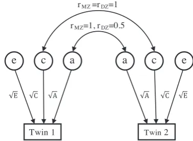
infer-ence. The SEM ACE model for univariate twin data can be displayed as a

path diagram, shown in Figure 1, where the influence caused by the latent

variablesa,c, andecan be described by the path coefficientspffiffiffiA,pffiffiffiffiCand

ffiffiffi

E

p

, respectively (Rijsdijk & Sham, 2002). According to path tracing

rules, the covariance matrices for MZ and DZ twin pairs are

CovMZ = A+C+E A+C

A+C A+C+E

!

,

CovDZ = A+C+E A=2 +C

A₌2 +C A+C+E

!

,

which have the same structure as matrices (4) and (5). The goodness

of fit of this model is also measured using the maximum likelihood

cri-terion (Rijsdijk & Sham, 2002). However, there exist some drawbacks

of this SEM approach employed in OpenMx for imaging data analysis.

The goodness-of-fit LRT statistic asymptotically follows a mixture of

chi-square distributions (Dominicus et al., 2006; Self & Liang, 1987;

Zhang & Lin, 2008), but we can observe that OpenMx incorrectly uses

a single standard chi-square distribution with 1 degree of freedom

(Rijsdijk & Sham, 2002). For neuroimaging, a relative weakness of

OpenMx is lack of direct tools for operating with neuroimaging data.

Solar

The sequential oligogenic linkage analysis routines (SOLAR) software

is designed for the investigation of genetic effects in imaging genetics

studies (Almasy & Blangero, 1998; Koran et al., 2014). In addition, the

SOLAR package is capable of estimating heritability with the data

from diverse family structures. SOLAR uses maximum likelihood to

estimate the variance parameters,A,C,E.To test the null hypothesis

of zero heritability, the LRT test statistic, which is asymptotically

dis-tributed as a mixture of chi-square distributions, can be calculated

(Almasy & Blangero, 1998). While SOLAR itself cannot read brain

imaging data, the related software SOLAReclipse (https://www.nitrc.

org/projects/se_linux) can read and write neuroimaging data.

2.3

|

Permutation inference

Permutation testing is a nonparametric technique that makes minimal

assumptions about the data. With a few simple assumptions like

exchangeability of the observed data under the null hypothesis, the

nonparametric permutation test is conceptually simple and

theoreti-cally intuitive (Nichols & Hayasaka, 2003; Nichols & Holmes, 2001).

When the null hypothesis is true, the data will exhibit the feature of

exchangeability, allowing permutation, re-fitting the model and

com-putation of the test statistic. With multiple permutations, an empirical

null distribution can be constructed and critical thresholds and p

-values computed. This approach has become feasible owing to the

widespread availability of powerful computers.

Applying variance component inference approach voxel-by-voxel

yields a test statistic image. For each voxel, if the null hypothesis of

no heritability, that is, H0:h2_{= 0, is assumed to be true, MZ and DZ}

twin pairs become exchangeable, allowing Np=

nMZ+nDZ

ð Þ=2

n_MZ=2

possible permutations of MZ and DZ labels on twin pairs. In the

pres-ence of nuisance covariatesX, residuals are permuted (here, as stated

above, we assume that the residualseapproximate the true errorsϵ).

Crucially, twin pairs stay linked, preserving any common environment

effects. As even moderate sample sizes can yieldNptoo large to allow

computing all permutations, in this case, an approximate or Monte

Carlo permutation test is conducted for a smaller number of

permuta-tions, sayNp= 1,000, based on a random subsample of all

permuta-tions (Nichols & Holmes, 2001).

In order to resolve the multiple comparisons problem and strictly

control false positives over the whole volume of regions of interest

(ROI's) or voxels simultaneously, a permutation test can also be used

to compute inferences corrected for the family-wise error (FWE).

FWE-correctedp-values are found by considering the null distribution

of maximum test statistics (Nichols & Holmes, 2001). With a

permuta-tion test, we obtain FWE-correctedp-values on peak height

(voxel-wise test statistic value) for voxel-(voxel-wise inference, and cluster size

(number of voxels involved in a cluster after thresholding) and cluster

mass (sum of voxel-wise test statistic values of all voxels within a

clus-ter afclus-ter thresholding) for clusclus-ter-level inference. Hence, this

permuta-tion approach can be further partipermuta-tioned into two parts: voxel-wise

single threshold test and cluster-wise supra-threshold tests.

2.3.1

|

Voxel-wise single threshold test

Let_π = 1,_…,Npbe the permutations considered including correctly

labeled data. At a single ROI/voxel, the permutation test produces a

level_αthreshold by finding thebαNpc+ 1 largest value of the null

dis-tribution;p-values are computed as the proportion of null distribution

values as large as or larger than the observed test statistic.

To control the FWE, the relevant null distribution is that of the

maximum test statistic. That is, the level-_αFWE thresholdTFWE

α is the

bαNpc+ 1 largest value of the maximum distribution, and

FWE-correctedp-value, denoted bypFWE

T , for any given test statisticT0is

likewise the proportion of permutation maximum distribution values

equaling or exceeding that value (Nichols & Holmes, 2001):

pFWE T =

# T_πmax≥T0

Np

,

whereTmax

π is elementπof the maximum distribution.

2.3.2

|

Cluster-wise supra-threshold tests

The significance of supra-threshold cluster tests can be assessed by the

spatially informed cluster statistics, such as cluster size and cluster

mass. A preselected cluster-forming threshold u, which can be

expressed as ap-value using the sampling distribution of the test

tic, is applied to the derived test statistic image to threshold test

statis-tic values and form supra-threshold clusters. A cluster sizeK, the count

of voxels in a cluster, or a cluster massM, the sum of test statistic

values exceedingu, can be computed. As clusters are random in number

and location, uncorrectedp-values can be found but reflect an

assump-tion of homogeneity over space and typically are not computed.

Computation of FWE-corrected inferences proceeds as with the

single-threshold test. ThebαNpc+ 1 largest element of the null

distribu-tion of maximum size (or mass) defines a critical level-_αFWE-corrected

thresholdKFWE

α (orMFWEα ). The associated FWE-correctedp-values are

pFWE_K =# K

max π ≥K0

Np

,

pFWE_M =# M

max π ≥M0

Np

,

for cluster statistics of size and mass, respectively, where K_πmax

(or M_πmax) is element _π of the maximum cluster size (or mass)

distribution.

3

|

S I M U L A T I O N S T U D I E S

In this section, univariate simulation analysis is conducted to compare

our newly proposed voxel-wise heritability estimation methods with

existing methods in terms of prediction accuracy, validity, sensitivity,

and the overall computation time for different variance component

settings. The ROC-based simulation studies generate 2D image data

for power evaluation and comparison between the voxel- and

cluster-wise heritability inference approaches for various settings.

3.1

|

Univariate simulation evaluations

We use Monte Carlo simulations to evaluate our proposed linear

regression methods, LR-SqD Perm (LR-SqD using empirical p-value

based on 1,000 permutations), LR-SqD (LR-SqD using asymptoticp

-value) and LR-SqD ReML, and existing methods including Falconer's

method, Bayesian ReML in SPM, SEM in OpenMx, and SOLAR.

3.1.1

|

Simulation setting

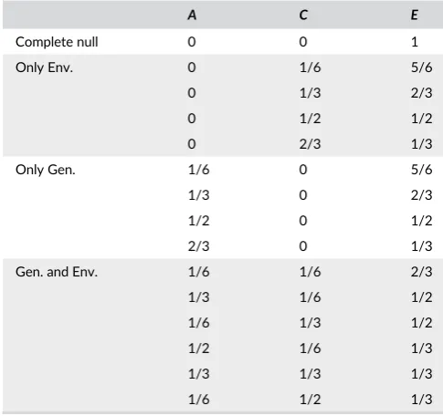
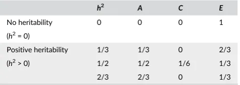
The parameter settings shown in Table 1 are motivated as follows. If we

create a 3D Cartesian coordinate system with x, y and z axes representing

the possible values forA,C,E, then the 3D parameter space can be

visual-ized as an equilateral triangle in 2D space utilizing a Barycentric

coordi-nate system, as shown in Figure 2. SinceEmax(A,C) usually holds in

practice, we choose 15 possible sets ofA,C,Efrom the upper part of this

parameter space satisfyingE≥1/3. Note that we assign values ofA,C,

Esuch thatA+C+E= 1, meaningAis directly interpretable ash2. That

is, the value ofAis exactlyh2. However, we still use

^

h2= A^

^

A+C^+E^

during computation to account for the genetic random variation in

For balanced design with an equal number of subjects for each

group (MZ and DZ twins), three samples are considered with the size

ofn= 100, 300, 1,000. For instance, the sample of 100 subjects is

comprised of 25 MZ twin pairs (50 subjects) and 25 DZ twin pairs

(50 subjects). For the unbalanced design, the sample size is fixed as

n= 300, and we consider the MZ:DZ ratios being 1:4 and 4:1, that is,

n= 60 + 240 andn= 240 + 60.

Apart from the Gaussian random error, we also take into account

the case where the error term is not normally distributed. Here we

consider a log-normally distributed unique environmental random

noise. The sample considered is balanced with the size ofn= 300,

that is, the number of MZ and DZ twin pairs is identical.

In total, 5 samples with balanced/unbalanced design and Gaussian/

non-Gaussian random error, along with 15 (A,C,E) parameter settings,

lead to totally 90 simulation settings. For each setting, we consider both

the one sample model (10) and multiple linear regression (15) to fit

SqD's. For the one sample model, no covariates are included in the

model (3) and the design matrix is an all-ones vector. For multiple linear

regression, age, sex, the interaction between age and sex and a standard

normally distributed continuous variable are included as covariates. The

regressors are simulated using Matlab.Xthus has five columns, in which

the first column is an all-ones vector for the intercept and the remaining

are randomly generated vectors approximating the four covariates.

Results are based on 1,000 realisations.

The mean squared error (MSE) is calculated to compare 6

estima-tion methods including LR-SqD, LR-SqD ReML, Falconer's method,

Bayesian ReML in SPM, SEM in OpenMx, and SOLAR. For each of all

seven testing (inference) methods considered (LR-SqD Perm, LR-SqD,

LR-SqD ReML, Falconer's method, Bayesian ReML in SPM, SEM in

OpenMx and SOLAR), we compute false positive rate (FPR), statistical

power, and overall running time. As the one sample model and

multi-ple linear regression model have qualitatively similar results, we will

only report the results obtained from multiple linear regression.

3.1.2

|

Comparison results

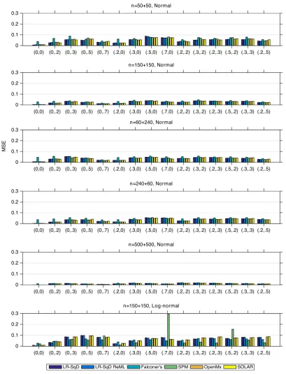
Accuracy and precision

The MSE comparison of six methods is shown in Figure 3, which

shows that the two linear regression methods, LR-SqD and LR-SqD

ReML, have MSE virtually identical to each other. For the first five

rows with Gaussian noise, with the exception of Falconer's method,

which generally has markedly worse MSE, all of the methods exhibit

roughly comparable MSE performance. For the sixth row with

non-Gaussian noise, the MSE of all methods is larger than that for Row

2 for nearly all parameter settings, and Falconer's method works

sometimes better and sometimes worse than the other methods.

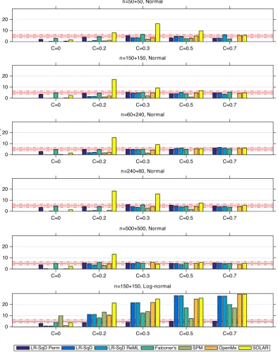
Specificity and statistical sensitivity

Figure 4 shows the specificity comparison of the seven testing

methods at a nominal significance level α = 0.05 (under the null

hypothesis of no heritability). With Gaussian noise (Rows 1_–5), when

the common environment effectCis also zero, all methods are highly

conservative except LR-SqD Perm and Falconer's, both of which are

close to exact for sufficient sample sizes. In the presence ofC> 0, the

methods are generally valid but SOLAR struggles, having inflated FPR.

We believe this is due to convergence problems for small samples.

For the non-Gaussian case (Row 6), we note that all methods are

inva-lid with inflated FPR except LR-SqD Perm, which does not rely on the

assumption of normality.

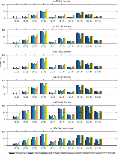
Figure 5 plots the power results. In the case of Gaussian noise, if

we set aside SOLAR's results that must be interpreted in light of its

inflated FPR, we find our linear regression methods using asymptotic

theoretical p-value and OpenMx have comparable power. LR-SqD

T A B L E 1 FifteenA,C,Eparameter settings

A C E

Complete null 0 0 1

Only Env. 0 1/6 5/6

0 1/3 2/3

0 1/2 1/2

0 2/3 1/3

Only Gen. 1/6 0 5/6

1/3 0 2/3

1/2 0 1/2

2/3 0 1/3

Gen. and Env. 1/6 1/6 2/3

1/3 1/6 1/2

1/6 1/3 1/2

1/2 1/6 1/3

1/3 1/3 1/3

1/6 1/2 1/3

F I G U R E 2 Parameter space with various (A,C, E) parameter

settings using Barycentric coordinates with barycenter (A,C,E) = (1/3,

1/3, 1/3). The large equilateral triangle (solid line) shows the ACE

parameter space with the constraintsA+C+E= 1,A, C,E≥0, where

the vertices (filled circles) represents the selectedA,C,Eparameter

settings shown in Table 1. The color of each vertex indicates the

Perm using permutation-based empirical p-values has the largest power in almost all settings, particularly for small values of heritability

and zeroCeffect. SPM's ReML method is generally less powerful.

Fal-coner's method is around the linear regression methods using

asymp-totic p-value and OpenMx, sometimes more, sometimes less

powerful. In the case of log-normally distributed random error (Row

6), we only consider LR-SqD Perm with controlled FPR. As expected,

the power is generally lower for all settings when compared with the

Gaussian case withn= 150 + 150 (Row 2).

Running time comparison

We evaluated the relative running time (relative to the running time

of Falconer's method) for completion of 1,000 simulated datasets (see

Figure 6). The computational performance comparing six methods

F I G U R E 3 The MSE comparison of LR-SqD, LR-SqD ReML, Falconer's method, Bayesian ReML in SPM, SEM in OpenMx, and SOLAR, based

on 1,000 realizations (Rows 1_–5 for Gaussian error and Row 6 for non-Gaussian error). Comma ordered pairs onx-axis correspond to the

rounded parameter values ofAandC, that is, (A,C); see Table 1 and Figure 2 for exact parameter settings used [Color figure can be viewed at

reveals that Falconer's method and the linear regression methods with

SqD's using asymptotic theoreticalp-values (i.e., LR-SqD and LR-SqD

ReML) always outperform other iterative methods including Bayesian

ReML in SPM, SEM in OpenMx, and SOLAR. For each simulation

set-ting, the overall computation time of all simulations for those

non-iterative methods is far smaller than the other non-iterative methods. The

LR-SqD Perm, based on 1,000 permutations, has running time

compa-rable to, or even longer than, those iterative methods. Nonetheless,

applying parallelization by running multiple jobs in parallel can help

reduce the overall computation time.

3.2

|

ROC-based power evaluation

To evaluate the sensitivity of the voxel- and cluster-wise heritability

inference approaches described in Section 2.3, we conduct a receiver

operating characteristic (ROC) analysis.

F I G U R E 4 The comparison of the estimated false positive rate (FPR) with a nominal level_α= 0.05 for true null hypothesis (H0:h2_{= 0, that is,}

A= 0), among LR-SqD perm using 1,000 permutations, LR-SqD, LR-SqD ReML, Falconer's method, Bayesian ReML in SPM, SEM in OpenMx, and

SOLAR, based on 1,000 realisations (Rows 1_–5 for Gaussian error and Row 6 for non-Gaussian error). Thex-axis represents the rounded values

ofC.The two red dash-dotted lines show the lower and upper bounds of the 95% binomial proportion confidence interval. The FPR should be

3.2.1

|

Simulation setting

In this set of simulations, we usen= 20, 60, 100, using only twins and

equal number of MZ and DZ pairs. The signal is generated with four

parameter settings shown in Table 2 consisting of different values of heritability and shared environmental variance.

The simulated images are 2D, with 128×128 pixels. Two spatial

configurations of signal were considered, a single large region or nine

separate regions, having similar number of signal pixels (1,020

vs. 1,024); see Figure 7. The set ofNIimages were first created by

fill-ing each pixel with i.i.d. standard Gaussian noise, and then inducfill-ing

the signal with the Cholesky decomposition of the desired

variance/covariance structure. Spatial Gaussian smoothing kernels

with full width at half maximum (FWHM) of 0, 1.5, 3, or 6 pixels were

applied to blur these images in order to accommodate spatial

F I G U R E 5 The statistical power comparison with a nominal level_α= 0.05 for false null hypothesis (H0:h2_{= 0) of LR-SqD Perm using 1,000} permutations, LR-SqD, LR-SqD ReML, Falconer's method, Bayesian ReML in SPM, SEM in OpenMx, and SOLAR, based on 1,000 realizations

(Rows 1_–5 for Gaussian error and Row 6 for non-Gaussian error). Comma ordered pairs onx-axis correspond to the rounded parameter values of

dependence across neighbouring voxels. A total ofNI= 1000 images were generated for each simulation setting.

3.2.2

|

ROC analysis

The ROC curves plot true positive rate (TPR; y-axis) against FPR

with varying threshold levels. A standard ROC analysis is suitable

for only a single outcome, while we have 1282 outcomes.

Hence we use an alternative, free-response ROC approach

(Chakraborty & Winter, 1990). As described in (Smith & Nichols,

2009), a free-response ROC, consisting of a y-axis representing

the probability of true detection, averaged over pixels withA> 0,

and anx-axis representing the probability of any false detections,

is deployed.

F I G U R E 6 The relative running time comparison after base-10 log transformation, denoted by log10(t/tF) for LR-SqD Perm using 1,000

permutations, LR-SqD, LR-SqD ReML, Bayesian ReML in SPM, SEM in OpenMx, and SOLAR, based on 1,000 realizations, wheretFdenotes the

running time for Falconer's method, that is, log10(t/tF) = 0 for Falconer's method (Rows 1_–5 for Gaussian error and Row 6 for non-Gaussian error).

Comma ordered pairs onx-axis correspond to the rounded parameter values of (A,C); see Table 1 and Figure 2 for exact parameter settings used

We summarize the ROC curve by a normalized area under the

curve (AUC), with a larger value for better performance. Since we are

mostly concerned about FPR values between 0 and 0.05,

corresponding to a family-wise error rate of 5%, the normalised AUC

is 20×AUC for FPR < 0.05, maintaining a“perfect”AUC of 1. We

cal-culate this free-response ROC curve for both voxel- and cluster-wise

inferences. For wise inference, we set the voxel-level

cluster-forming threshold toα= 0.05 or LRT statistic valueuα= 2.71.

For clarity, the exact steps in this ROC calculation are as follows.

1. GenerateNI= 1000 i.i.d. 2D smoothed null images with standard

Gaussian random noise, where (A, C, E) = (0, 0, 1), and the

corresponding smoothed heritability signal images, where the

sig-nal were generated with (A, C, E) as per one configuration in

Table 2, and one of two spatial configurations in Figure 7.

2. For each image, estimate heritability pixel-by-pixel and create the

LRT test statistic image.

3. Voxel-wise inference.Apply a large number of predefined grids of thresholds to the LRT test statistic image, obtain the

supra-threshold pixels, and then calculate family-wise FPR and TPR for

each of these threshold levels, obtaining FPR from noise-only

image and TPR from theA> 0 pixels in signal images.

Cluster-wise inference.Threshold the LRT statistic images with a

predetermined cluster-forming threshold (p-valueαor statisticuα)

and form clusters. Use a predefined grid of cluster size thresholds

to define each cluster as detected or not.

4. Compute the family-wise FPR and TPR:

FPR.Using the smoothed random noise images, for each threshold,

the family-wise FPR is the proportion of realizations having any

(false) detections.

TPR.Using the heritability images, for each threshold, compute the

proportion of true positive pixels (detected andA> 0) out of all

possible (number of theA> 0 pixels). This is computed for each

realization and averaged over realizations.

5. Plot the ROC curves and calculate the corresponding normalized

AUC values.

3.2.3

|

ROC-based simulation results

As described above, a range of simulation settings are investigated for

both voxel- and cluster-wise inference approaches using APACE. For

different extents of smoothness, the returned ROC curves have fairly

similar shape, so we will only illustrate the ROC curves created by

medium degree of smoothing with FWHM of three pixels, which are

shown in Figures 8 and 9 for the simulated focal and distributed

sig-nals, respectively. The corresponding normalized AUC comparison is

then shown in Figure 10.

For both focal and distributed signal, ROC curves of the

cluster-wise method are always above those of the voxel-cluster-wise method,

reflecting higher statistical power obtained for cluster- than

voxel-wise inference approaches. In general, for a particular family-voxel-wise FPR

level, the TPR value of both inference methods becomes larger when

the sample size or the heritability is increased.

The normalized AUC values (Figure 10) show that the voxel-wise

method has poor performance overall for all simulation settings with

negligible AUC values, while the cluster-wise inference approach has

much larger AUC values. While the absolute power is low here,

reflecting the challenge of detecting nonzero heritability with just

100 subjects, these results show that the cluster-wise approach is

more sensitive to such spatial signals and demonstrates the value of

such spatial statistics.

4

|

R E A L D A T A A N A L Y S I S

Here we report the heritability analysis of a working memory fMRI

task. We illustrate the above-mentioned heritability inference

approaches including univariate LR-SqD and permutations.

T A B L E 2 Four parameter settings of heritabilityh2and

parametersA,C,E

h2 _{A C E}

No heritability 0 0 0 1

(h2_{= 0)}

Positive heritability 1/3 1/3 0 2/3

(h2_{> 0) 1/2 1/2 1/6 1/3}

2/3 2/3 0 1/3

4.1

|

Real data acquisition

The experimental sample comprisesn= 319 young and healthy

partic-ipants from Queensland, Australia (199 females and 120 males),

con-sisting ofnMZ= 150 MZ twins (75 pairs with 46 female and 29 male

pairs), nDZ= 132 DZ twins (66 pairs with 30 female, 11 male, and

25 opposite sex pairs) and nS= 37 unpaired twins (22 female and

15 male). The age range of all these subjects is 20_–28 years (mean

±SD: 23.6 ± 1.8). A 4T Bruker Medspec full-body scanner was utilized

and task-related fMRI BOLD was acquired while participants

per-formed a block design n-back task, consisting of 0-back and 2-back

conditions. Imaging preprocessing was implemented using SPM5

soft-ware in Matlab, including image realignment with a mean image

gen-erated, spatial normalization to the standard T1 template in MNI atlas

space, spatial smoothing with an isotropic Gaussian kernel, removal of

global signal effects, and the use of high-pass and low-pass filtering to

discard uninterested signals. For each subject, the brain activation,

measured as the 2-back >0-backt-contrast images using a one-sample

t-test, was extracted. Only areas of expected activation in the frontal

and parietal regions are included in the mask, comprised of 14,627

voxels in total. Age, sex, and 2-back performance accuracy (the

per-centage of correct responses) are included as the covariates in the

sta-tistical analysis (Blokland et al., 2011).

4.2

|

Real data results

The permutation-based empirical distribution of maximum LRT

statis-ticT_πmaxgives 5% FWE threshold ofTFWE_α = 11:32, and for the

cluster-wise results, the 5% FWE thresholds of maximum supra-threshold

cluster sizeKmax

π and maximum supra-threshold cluster massMπmaxare

KFWE

α = 62 and MFWEα = 271:74, respectively. The most significant

FWE-correctedp-values are 0.007, 0.001, and 0.001 for voxel, cluster

size and cluster mass statistics, respectively.

The supra-threshold cluster tests found much larger significant

brain regions than the single threshold test by comparing their

FWE-correctedp-value images. For the voxel-wise single threshold test,

F I G U R E 8 The ROC curve comparison of voxel- (“V,”dashed

lines) and cluster-wise (_“C,_”solid lines) inference approaches for three

settings of (A,C,E) = (0.3, 0, 0.7), (0.5, 0.2, 0.3), (0.7, 0, 0.3),

corresponding toh2_{= 0.3, 0.5, 0.7, for the focal signal with three}

sample sizes of 10 + 10 (upper), 30 + 30 (middle) and 50 + 50 (lower),

where_“V-0.3_”and_“C-0.3_”represent the settings of voxel-wise

inference andh2= 0.3 and cluster-wise inference andh2= 0.3,

respectively [Color figure can be viewed at wileyonlinelibrary.com]

F I G U R E 9 The ROC curve comparison of voxel- (“V,”dashed

lines) and cluster-wise (_“C,_”solid lines) inference approaches for

3 settings of (A,C,E) = (0.3, 0, 0.7), (0.5, 0.2, 0.3), (0.7, 0, 0.3),

corresponding toh2_{= 0.3, 0.5, 0.7, for the distributed signal with}

three sample sizes of 10 + 10 (upper), 30 + 30 (middle) and 50 + 50

(lower), where_“V-0.3_”and_“C-0.3_”represent the settings of

voxel-wise inference andh2= 0.3 and cluster-wise inference andh2= 0.3,

F I G U R E 1 0 The normalized AUC (20×AUC for FPR = 0:0.05) comparison of voxel- and cluster-wise inference approaches for different (A,

C,E) parameter settings, three samples of sizen= 10 + 10, 30 + 30, 50 + 50, and two tested signals (focal and distributed) with positive

heritabilityh2> 0 [Color figure can be viewed at wileyonlinelibrary.com]

F I G U R E 1 1 The log-transformed

FWE-correctedp-value image, that is,

−log10 pFWEK

only two significant voxels were identified, while there were four

clus-ters with a total of 634 voxels identified to be significant for the

cluster-wise tests. The FWE-corrected p-value image after log-10

transformation, that is,₋log10(pFWE_{), for significant supra-threshold}

clusters with respect to size statistic is shown in Figure 11. The

herita-bility estimate image is shown in Figure 12, where the heritaherita-bility

esti-mate ranges between 0 and 0.59, and the significant voxels based on

cluster-wise inference have a heritability range of 0.18 and 0.59. The

most heritability-significant regions found using both the single

threshold test and the supra-threshold cluster tests overlap with the

most significant regions from the previous Mx analysis (Blokland

et al., 2011).

5

|

C O N C L U S I O N A N D D I S C U S S I O N

In this article, we have presented two novel linear regression-based

estimation methods for heritability inference in neuroimaging, trying

to improve statistical power and reduce computational complexity. A

simple LR-SqD method based on linear regression modeling with

squared differences of paired observations has been developed, and

found to have comparable or even better estimation accuracy and

sta-tistical power relative to existing methods. LR-SqD, as simple as

Fal-coner's method, only requires linear regression to improve prediction

accuracy. The univariate simulation study also showed that apart from

Falconer's method, LR-SqD is the most time-efficient approach when

compared with those likelihood-based iterative methods, and will

never encounter any convergence problems. The fast, accurate and

noniterative properties of LR-SqD make it more flexible and feasible

to be applied for permutation inference.

A permutation-based heritability inference approach by

embed-ding LR-SqD method in a permutation framework has also been

devel-oped. This permutation inference allows us to perform more exact

heritability inference using LR-SqD Perm at each voxel, to control the

FWER, and also to consider alternative cluster-wise imaging statistics.

The fact that adjacent voxels or regions in a brain image tend to be

structurally and functionally homologous can be exploited by spatial

statistics like cluster size and mass. Our use of LR-SqD, the fast and

accurate noniterative method (free of any convergence issues), makes

these spatially informed statistics more accessible. For equivalent

FWERs, the cluster-wise approach was found to have higher

sensitiv-ity, and thus more powerful in ROC-based power simulations, which

demonstrates the importance of such spatial statistics over voxel-wise

statistics and the need for permutation inference to take advantage of

these cluster statistics. With few weak assumptions, permutation

inference is a feasible alternative to the parametric approaches, which

is even preferable in studies having small sample sizes or when the

stronger assumptions of the parametric approaches cannot be met

(Nichols & Holmes, 2001).

Except for LR-SqD Perm, methods being compared in univariate

simulations are asymptotic. We found our permutation-based LR-SqD

method, LR-SqD Perm, is more robust, being the most powerful

approach for nearly all simulation settings. Other asymptotic LR-SqD

methods, LR-SqD and LR-SqD ReML, also have good power, and cluster

inference methods have better detection power than voxel-wise

methods. A sample size of 1,000 is still insufficient, for some parameter

settings, resulting in limited power (far below 80%) for detecting

herita-bility, but at least we found all methods are valid with normally

distrib-uted errors except SOLAR, which is specially designed for family studies

with large sample sizes of various degrees of relatedness. For Gaussian

noise, although Falconer's method has poor estimation accuracy, it

seems to work well with the power comparable to that of LR-SqD Perm.

However, it relies on the normality assumption to test for the

equiva-lence of MZ and DZ correlations. For non-Gaussian noise, the null

distri-bution of LRT computed under the misspecified normality assumption

can be inaccurate and the corresponding asymptotic null distribution of

LRT based on Wilk's theorem is problematic, which results in inflated

FPR as shown in our simulations. LR-SqD Perm, which relaxes the

assumption of normality, is the only applicable method that maintains

valid FPR control in the case of non-Gaussian error, and thus we

sug-gest sticking to LR-SqD Perm. During univariate evaluations, we found

adding singletons can improve neither estimation accuracy nor

cal power. However, we still suggest including singletons in the

statisti-cal analysis since a better estimate of the phenotypic variance can be

obtained with more data taken into account. Averaging across all the

simulation settings, we found LR-SqD is roughly 2.5 times faster than

LR-SqD ReML, and around 45.5, 84.8, and 995.7 times faster than

SPM, OpenMx and SOLAR, respectively.

The LRT statistic for testing H0:A= 0 is not asymptotically pivotal

and its distribution varies discontinuously across the parameter space

depending on the true value of variance componentC.The

configura-tions ofCon the parameter space can be partitioned into two cases:

(1)C> 0, (2)C= 0. For standard Case (1), the reference distribution for

the LRT involving one parameter on the boundary of the parameter

space has been proven to be a half-half mixture ofχ2

0andχ21(Dominicus

et al., 2006; Self & Liang, 1987). For nonstandard Case (2), under the

null, bothAandCare boundary parameters and the asymptotic

distri-bution of the LRT statistic is a mixture of_χ2

0,χ21, andχ22with mixing

probabilities 1/2−p, 1/2 andp, where 0≤p≤1/2 (Dominicus et al.,

2006; Self & Liang, 1987). Even ifC> 0 for Case (1), the asymptotic

null distribution of the LRT statistic for a finite sample can be more

sim-ilar to that for Case (2) whenCis close enough to the boundary (Self &

Liang, 1987). When the sample size tends to infinity or is sufficiently

large, the asymptotic approximation is enhanced, and the tendency

eases with the reference distribution more resembling that for Case (1).

This leads to the conservativeness of the asymptotic LRT-based tests

when compared with the permutation-based LR-SqD Perm, and thus

we recommend using the nonparametric permutation inference.

The existence of nonzero variance componentsAandCinduces

the familial correlation (Dominicus et al., 2006). When the true value

ofAis nonzero, testing the null hypothesis of no heritability is similar

to testing for the familial correlation since it would be difficult to

pre-cisely separate the familial influences and explicitly distinguish

between theAandCeffects due to the inevitable noise, which has

been revealed in univariate simulation evaluations. Therefore,

increas-ing the variance parameterCmay improve the power of the test for

the null hypothesis of no heritability while holding the validity of the

test. In addition, whenC is zero, the test comparing the AE model

against the E model could probably offer higher power than the test

of ACE versus CE. However, the variance parameterCis unknown in

reality and impulsively using the test of AE versus E would lead to

inflated FPR and invalid conclusions with overestimated power.

We have developed a Matlab-based tool“Accelerated Permutation

Inference for the ACE Model (APACE)_”, which provides different

analy-sis approaches specialized for heritability inference based on LR-SqD

and is freely available at https://github.com/NISOx-BDI/APACE.

Com-pared with the popular analysis tools such as OpenMx and SOLAR,

APACE is designed specifically for neuroimaging data and is applicable

for any sample sizes with controlled FPR. The use of the flexible

permu-tation approach allows for any test statistics (e.g., LRT, cluster size, and

so on) to be applied in computing thep-values, and enabling parallel

execution further accelerates the implementation. The current version

of APACE can be adopted for the family design including twins, siblings

and singletons, and the generalization of APACE for any family designs

is possible with the use of the pedigree information.

A C K N O W L E D G M E N T S

This work was supported by Technology Foundation STW (project

no. 12724 to E.F.), the Dutch Province of Limburg (MaCSBio), and

National Institutes of Health (K99AG054573 to T.G.). The n-back fMRI

data were acquired as part of the Queensland Twin Imaging Study. The

QTIM study is an ongoing longitudinal study of healthy young twins

with structural and functional MRI, diffusion tensor imaging, genetics,

and comprehensive cognitive assessments (de Zubicaray et al., 2008).

This study was supported by grant number R01HD050735 from the

Eunice Kennedy Shriver National Institute of Child Health and Human

Development, USA, and Project Grant 496682 from the National

Health and Medical Research Council (NHMRC), Australia. Zygosity

typ-ing was supported by the Australian Research Council (ARC;

A7960034, A79906588, A79801419, and DP0212016). The content of

this article is solely the responsibility of the authors and does not

neces-sarily represent the official views of the Eunice Kennedy Shriver

National Institute of Child Health and Human Development, NIH,

NHMRC, or ARC.

D A T A A C C E S S I B I L I T Y

We have developed a Matlab-based tool“Accelerated Permutation

Inference for the ACE Model (APACE)”, which provides different

anal-ysis approaches specialized for heritability inference based on LR-SqD

and is freely available at https://github.com/NISOx-BDI/APACE.

O R C I D

Xu Chen https://orcid.org/0000-0001-9506-1815

Gabriëlla A. M. Blokland https://orcid.org/0000-0003-0566-444X