FUZZY OPTIMIZATION USING
EXTENDED KALMAN FILTER
S.VIJAYACHITRA
Professor, Department of Electronics and Instrumentation Engineering Kongu Engineering College, Perundurai
Erode, Tamilnadu [email protected]
M.DIVYA
PG scholar, Department of Electrical and Electronics Engineering Kongu Engineering College, Perundurai
Erode, Tamilnadu [email protected] Abstract :
Fuzzy Logic is based on the idea that in fuzzy sets each element in the set can assume a value from 0 to 1, not only 0 or 1, as in crisp set theory. The degree of membership function is defined as the gradation in the extent to which an element is belonging to the relevant sets. Optimizing the membership functions of a fuzzy system can be viewed as a system identification problem for nonlinear dynamic system. In this paper two input and one output fuzzy controller is designed for the dynamic process of aircraft. The addition of an EKF in the feedback loop improved the system response by blocking possible effects of measurement error based on Predictor-Corrector algorithm. An Extended Kalman Filter approach to optimize the membership functions of the inputs and outputs of the fuzzy controller. The performance of the fuzzy system before and after the optimization are compared, as well as the membership functions.
Keywords: Fuzzy controller, Extended Kalman Filter, Optimization. 1. Introduction
The performance of a fuzzy system depends on both its rule base and its membership functions. Given a rule base, the membership functions can be optimized in order to obtain the best performance from the fuzzy system. Tao and Taur designed an adaptive fuzzy controller for new rule insertion based on the design requirements [9].Wu and Chen presented a new fuzzy learning algorithm to get a better accuracy rate based on α cuts of equivalence relations [10].Dan simon modified the optimization approach to obtain the resulting memberhip functions are sum normal . Jacomet created a penalty function to obtain the optimization algorithm [4].
The filtering is the vital problem in many processes. When the system is linear; the Kalman filter can be used in a simple way to obtain the solution. But most of the process are non linear and complex in nature. So the Kalman filter cannot be used directly. A Kalman filter is a probability-based digital filter capable of filtering "white noise," which is containing the entire frequency spectrum. Kalman filter is a recursive predictive filter that is based on the use of state space techniques and recursive algorithms [3]. This method is originally developed for use in spacecraft navigation , but nowadays the Kalman filter turns out to be useful for many applications.
Most of the processes in real life are not linear and therefore needs to be linearized before they can be estimated by means of Kalman filter. The nonlinear function can be estimated around the current estimate using the partial derivatives of the process and measurements functions to be compute estimates in the fact of nonlinear relationships. Extended Kalman Filter algorithm resembles the predictor-corrector algorithm [6].
In this paper we presented the fuzzy controller with two input and one output. Membership function of the fuzzy controller inputs and output are optimized using extended Kalman filter approach. The performance of fuzzy controller are compared before and after the optimization,as well as membership functions.
2. Fuzzy membership function and its parameters
In this paper we will assume five membership functions are available in each input and output of the fuzzy controller. In that five membership functions first and last membership functions are trapezoidal.
Other three membership functions are triangular. We denote the centroid, lower half width, and upper half width of the ith fuzzy membership function of the jth input by
c
ij,b
ij ,
b
ij
0
( )
0
ijij ij ij ij ij ij
ij ij ij ij ij
ij
x
b
x b
b
b
b
x
b
F x
c
x c
b
b
x
c
x
c
. (1)
Similarly for a single output fuzzy system, we denote the centroid and half width of the fuzzy membership function of the output by and respectively. In two input and one output fuzzy system ,the fuzzy output is mapped into a crisp value using centroid defuzzification.
Crisp output= 1
1
(
)
(
)
n
j j j j n j j j
m
m
. (2)where n is the number of fuzzy output sets.the fuzzy output function m(
) is computed as follows: m(
)=fuzzy output function=,
( )
ik i km
. (3)where
m
ik(
) is defined as consequent fuzzy output function when (input 1
class i) and (input 2
class k).ik
m
(
)=w m
ik oik(
). (4)oik
m
(
) is the fuzzy function of the consequent that is activated when (input 1
class i)and (input 2
class k). andw
ikis the activation level of that consequents.ik
w
=min
f input
i1(
1),
f
k2(
input
2)
. (5)Since the fuzzy membership functions are trapezoidal as assumed,derivative-based methods can be used to optimize the centroid and half widths of the input and output membership functions. Consider the error function given by
2 1
1
2
N q qE
N
E
. (6)ˆ
q q qE
y
y
. (7)Where N is the number of training samples,
y
q is the target value of the fuzzy system, andy
ˆ
q is theoutput of the fuzzy system. 3. Extended Kalman filter
In the Extended Kalman Filter, the state transition and observation models need not be linear functions of the state but may instead be differentiable functions. Consider a nonlinear dynamic model given as follows[5]:
1 1 1
(
,
)
k k k k
x
f x
u
w
(8)(
)
k k k
z
h x
v
(9)where the process and observation noises are denoted by wk and vk ,here both assumed to be zero mean
multivariate Gaussian noises with covariance Qk and Rk respectively.
Predict
Predicted state estimate
ˆ
(
ˆ
,
)
Update
Innovation or measurement residual
/ 1
ˆ
(
)
k k k k
y
z
h x
(12) Innovation (or residual) covariance/ 1
T k k k k k k
S
H P
H
R
(13) Near-Optimal Kalman gain1
/ 1
T k k k k k
K
P
H S
(14) Updated state estimate/ / 1
ˆ
k kˆ
k k kˆ
kx
x
K y
(15) Updated estimate covariance/
(
)
/ 1k k k k k k
P
I
K H
P
(16)
where the observation matrices and state transition are defined to be the following Jacobians matrices
1/ 1, 1
ˆ
1
/
k k kk x u
f
F
x
(17)/ 1
ˆ
/
k k
k x
h
H
x
(18)After finding the jacobian matrices, the EKF computes time update equations and measurement update equations.
The steps for computing time update equations are: 1.project the state ahead
1 1 1
ˆ
(
ˆ
,
, 0).
k k k
X
f x
u
(19)2.project the error covariance ahead
1 1
T T
k k k k k k k
P
A P A
W Q W
. (20)The time update equations project the state and covariance estimates from the previous time step k-1 to the current step k.
A
kandW
k are process jacobians at step k,andQ
k is the process noise covariance at step k. 4. Implementation and experimental resultsConsider the Dynamic process of Aircraft plant given as follows[5]:
Mv= ((α*V)+(β *(V).^3))+
k
e*
-m*9.8*sin(GRAD) (21)Where mass of the aircraft m=800kg,drag coefficients α =100N/(m/sec) and β=0.01
N
/ (
m
/ sec)
3 ande
k
is 4000 Newtons. v is the velocity of the plant ,
is the throttle position ,and grad is a variable has a 15 percent positive increase. The plant is expected to maintain the velocity at 70 m/s. The plant should converge as fast as possible at the velocity 70m/s unless there is another change.System speedy: 2 inputs, 1 outputs, 25 rules e (5)
ce (5)
f (u)
speed (5) speedy
(sugeno)
25 rules
Each membership function of an input has three parameters i.e. centroid, lower half width and upper half width to determine , and output membership function has two parameter i.e.centroid and half width to determine. Table .1.shows the rule base implementation.
Table 4.1: Fuzzy rule base
e Ce
NL NS Z PS PL
NL NL NL NL Z PS
NS NL NS NS Z PS
Z NS Z Z Z PS
PS NS Z PS PS PL
PL NS Z PL PL PL
PS=Positive Small, PL=Positive Large, NL=Negative Large, NS=Negative Small, Z=Zero.
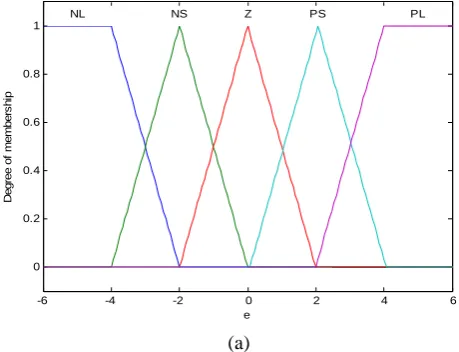
To optimize the membership function of the fuzzy controller inputs and output, the Extended Kalman Filter method is implemented. The membership function of input1 (e), input2 (ce) and output before the optimization are shown in Fig.2(a), Fig.2(b) and Fig.2(c) respectively.
-6 -4 -2 0 2 4 6
0 0.2 0.4 0.6 0.8 1
e
D
egr
e
e
o
f m
e
mb
er
s
h
ip
NL NS Z PS PL
-6 -4 -2 0 2 4 6 0
0.2 0.4 0.6 0.8 1
ce
D
e
gr
ee
o
f
m
e
m
be
rs
h
ip
NL NS Z PS PL
(b)
-0.5 -0.4 -0.3 -0.2 -0.1 0 0.1 0.2 0.3 0.4 0.5 0
0.2 0.4 0.6 0.8 1
speed
D
egr
ee of
m
em
b
er
s
hi
p
NL NS Z PS PL
(c)
Fig 2.(a) The membership function of input1 before the optimization.(b)The membership function of input2 before the optimization.(c)The membership function of the output before the optimization
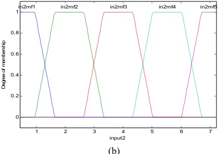
The membership function of fuzzy controller inputs and output are compared before and after optimization. The membership function of input1,input2 after optimization are shown in Fig.3(a),and Fig.3(b) respectively
.
1 2 3 4 5 6 7
0 0.2 0.4 0.6 0.8 1
input1
D
egr
ee of
m
em
ber
s
hi
p
in1mf1 in1mf2 in1mf3 in1mf4 in1mf5
1 2 3 4 5 6 7 0
0.2 0.4 0.6 0.8 1
input2
D
egr
ee
o
f
m
e
m
ber
s
h
ip
in2mf1 in2mf2 in2mf3 in2mf4 in2mf5
(b)
Fig 3.(a) the membership function of input1 after the optimization. (b) the membership function of input2 after the optimization
Fig.4 shows the training error of the Extended Kalman Filter during the optimization of the membership functions. The training error gets converged at 250th iteration. The extended Kalman filter which resembles the predictor-corrector algorithm is used to optimize the membership function of fuzzy controller
.
The training error is defined as the difference between the training data value and the output of fuzzy inference system training data value.
Fig.4 Error Curves
5.Conclusion
Here the Extended Kalman Filter is the non linear version of the Kalman filter are used to optimize the membership function of fuzzy controller which is having two input and one output system. The method was applied to a non linear dynamic process of the plant which is given in the mathematical form. for this non linear process fuzzy controller was designed and based on the membership functions rules are generated. In this system the extended Kalman filter is used as the estimator to predict the appropriate output. This method gives the better estimation and it converges quickly.
References
[1] Dan Simon(2002), “Training Fuzzy Systems With The Extended Kalman Filter,” Fuzzy Sets And Systems, FSS 3806,pp. 1-11. [2] D.Drainkov,H.Hellendoorn(1993), “ An Introduction To Fuzzy Control.” Berlin Germany:Springer –Verlang.
[3] Greg Welch and Gray Bishop(2001), “An Introduction To The Kalman Filter,” ACM SIGGRAPH.
[4] Jacomet, Stahel, Walti (1995), ‘On-Line Optimization Of Fuzzy System’, Konferenzartikel 2nd Annual Joint Conference on
Information Sciences,Wrightsville Beach,pp-301-313.
[5] John Yen and Reza Langari(1999), “Fuzzy Logic :Intelligence, Control And Information,”Prentice Hall,ISBN:0-13-525817-0. [6] R.E.Kalman(1960), “A New Approach To Linear Filtering And Prediction Problems,” Transaction of the ASME –Journal Of Basic
Engineering ,82(series D), pp. 35-45.
[7] Mohinder S.Grewal and Angus P.Andrews(1993), “Kalman Filtering Theory And Practice,” Prentice Hall. [8] Timothy J.Ross(1995), “Fuzzy Logic With Engineering Applications” ,McGraw-Hill,ISBN:0-07-053917-0.
[9] C.Tao and J.Taur(1999), “Design Of Fuzzy Controllers With Adaptive Rule Insertion” IEEE Transaction On Systems,Man And Cybernatics,Part B, vol. 29, pp. 389-397.