PREDICTION OF COMBUSTION
CHARACTERISTICS OF A TYPICAL
BIOGAS BURNER USING CFD
K. MADHUSOODAN PILLAI
Formerly Associate Professor, T. K. M. College of Engineering,
Kollam 691005, Kerala. madhutkmce@gmail.com
MADHU G.
P G Scholar,
Department of Mechanical Engineering, T. K. M. College of Engineering,
Kollam691005, Kerala. mgckm@yahoo.co.in
Dr. K. E. REBY ROY
Assistant Professor,
Department of Mechanical Engineering, T. K. M. College of Engineering,
Kollam691005, Kerala, rebyroy@yahoo.com
Abstract:
Biogas is obtained from anaerobic digestion of biodegradable materials such as agricultural waste, animal waste, and othertype of household solid waste and its main constituents are CH4 and CO2. Effects of the concentration of each species are very important in the biogas combustion. The present study focuses on the effect of inlet velocities of methane and air on the flame temperature in a biogas burner lamp. The model of biogas burner lamp is constructed by using the CFD software GAMBIT and the simulation process was performed by using Fluent Software. The flame temperature obtained is 2172 k when the inlet velocities of methane and air are 0.2m/s and 0.8 m/s respectively. Results of this study will provide valuable data for biogas burner lamp manufacturers.
Keywords: Biogas combustion; adiabatic flame temperature; volumetric combustion.
1. Introduction
It has become understand that mankind’s use of fossil fuels has made unsustainable problems on the planet. As mentioned in the IPCC report [1], the warming of the climate conditions is undeniable—manifested in observations of rising global average air and ocean temperatures, extensive melting of ice andsnow, and a global average sea level on the rise. In 2004, 56% of greenhouse gases emitted by mankind were carbon dioxide from fossil fuels [1]. When these fossil fuels are burned, the carbon dioxide is released into the atmosphere after having been trapped from the carbon cycle, which is the path carbon follows as it passes through our living area [1]. This process places extra problems on a system that is already operating in equilibrium, producing global warming.
released when burned is that which the plant matter absorbed from the atmosphere to begin with.The required technologies for burning biogas, in place of fossil fuels can be developed. Although the production of biogas is well clear, the effective combustion of the substance is very problematic. A better understanding of the methods available and the processes that take place during the combustion is required to remedy these problems. There mainly two approaches to improving our knowledge in this area suggest themselves: the use of empirical data collected by burning the biofuel and the development of a computational fluid dynamics model (CFD).
1.1 Objectives
This work has mainly two-part objective. One is to employ CFD to make a numerical biogas-airflow model of a biogas burner lamp. The second part is to validate the model using theoretical and empirical details available from previous studies and collected from the physical burner. Finally the model should be useable for eventual integration with a biogas combustion model for use in predicting the behaviour of full scale industrial burner lamp running on biogas.
1.1 Literature survey
A.F. Brancelli1 et al.[2] studied theParametrical Analysis of a Biogas Fuel Combustion Process in a Chamber in Steady-State Condition. Their work represents a typical CFD application related to a combustion process with hydrogen rich fuel in standard operative conditions on a Sandia-like burner. The influence of burner geometry and the gas velocity have been studied in order to predict the better conditions for an efficient combustion with low pollutant realised in steady state.
Y. Lafay et al.[6]., discussed theExperimental study of biogas combustion using a gas turbine configuration. In this the aim of their work is to compare stability combustion domains, flame structures and dynamics between CH4/air flames and a biogas/air flames in a lean gas turbine premixed combustion conditions.
SaeedJahangirian and Abraham Engeda[4], studied the Biogas combustion and chemical kinectics for gas turbine applications. Combustion characteristics such asignition delay kinetics study and GRI-Mech 3.0 detailed kinetics times and laminar flame speeds were investigated and characterized for fuel blends of diluted methane that simulate biogas with variable compositions using a systematic chemical mechanism. Correlations were found to predict the behaviour of individual diluents (CO2 or N2) in a biogas.
Carlos Díaz-González1 et al,[3], studied the Comparison of Combustion Properties of Simulated Biogas and Methane. The combustion properties of a simulated gas composed of 60% methane and 40% carbon dioxide in volume are determined by means of calculation algorithms developed by the GASURE team, comparing them to pure methane properties.
AhamadSakhrieh[5], investigated the Effect of pressure and inlet velocity on the adiabatic flame temperature of a Methane –Air flame.These study focuses on the effect of pressure and high inlet velocity of turbulent premixed flames on the adiabatic flame temperature of a methane-Air Flame.
1.2 Volumetric combustion
The idea of the volumetric combustion has been introduced by Prof. Blasiak[7]. The characteristics of volumetric combustion are very intensive mixing and internal recirculation inside of the combustion chamber. In this case, combustion occurs in a very higher volume with relatively uniform distribution of reacting species, temperature and heat fluxes. Theidea is later developed a new combustion concept for a 100% pulverized biogas combustion in a boiler. In order to control the combustion process of biomass in boiler, the properties of wood pellets combustion in high temperature oxidizer wereanalysed.In the case of volumetric combustion a volume of the fuel and oxidizer is introduced into the combustion chamber..
2 CFD Analysis
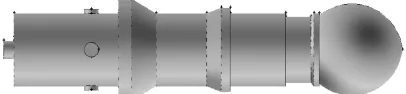
The figure1 has shown below shows the typical biogas burner lamp. The design is selected from Dr. David Fulford’s design of biogas burner lamp[8]. The burner body is assumed to be insulated. It consists of mainly five parts. Theyare,
(1) A long fuel –air mixing tube
(2) Four number of air inlet ports
(4) A mantle for lighting
(5) A jet with internal needle
Fig. 1. Schematic diagram of a biogas burner lamp
2.1
Model illustrationThe diagram of the biogas burner lamp is shown in figures 2 and 3, which are constructed by using GAMBIT software. Figure 2, shows the meshed view of the model.The analysis software used here Fluent 6.3. The element type used for mesh generation is TET/HYBRID. Total number of elements is 897448.
Segregated solver is used for the present work. The governing equations are solved sequentially in segregated solver and the turbulence model used in the present study is k- ε model. The combustion is modelled using the volumetric option available with FLUENT.
Fig. 2 Diagram of biogas burner lamp constructed by GAMBIT 2.4.6
Fig. 3.Meshed view of biogas burner lamp
3 Results and discussions
velocity of air flow istaken as constant which is equal to 0.8 m/s. and the inlet velocities of methane are 0.1m/s, 0.2m/sand 0.3m/s, respectively. Also the mass fractions of methane and oxygen are considered to be 0.8 and 0.21 respectively. All the cases the temperature is increased, however theoptimum inletvelocities of air and methane are 0.8m/s and 0.2 m/s respectively. In this case only the methane content in the combustion chamber is too small compared to the other two cases, that means the unburned methane is very less.
3.1 Case-1.
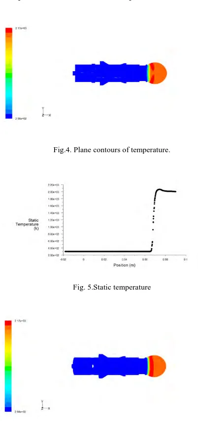
In this case the inlet velocities of methane and air are considered as 0.1m/s and 0.8m/s respectively.The following figure4, represents the plane contours of temperature. From the figure we can say that the maximum temperature obtained is 2165k and then slightly decreases. The graph,figure 5,shown below indicates the static temperature with position, and which shows the temperature increases and reaches a maximum of 2165k and then slightly decreases.Figure 6, represents the contours of temperature in the actual geometry.
Fig.4. Plane contours of temperature.
Fig. 5.Static temperature
Fig. 6. Contours of temperature of actual geometry
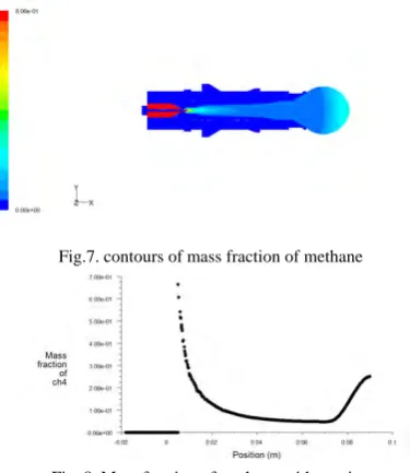
Fig.7. contours of mass fraction of methane
Fig. 8. Mass fraction of methane with postion
The following figure 9, shows the plane contours of mass fraction of oxygen and from the figure we can see that the masss fraction of oxygen is increasing from the inlet and at the mantle position the quantity of oxygen is very less. The graph, figure 10, shows the mass fraction of oxygen with position and from this graph we can understand the outer portion has less oxygen content.
Fig. 9. Contours of mass fraction of oxygen
Fig. 10. mass fraction of oxygen with position
The figure 11, shown below indicates the contous of mass fraction of Carbondioxide and the graph, figure 12, represents the same with position. Initially the quantity is zero and when the combustion started the quantity of CO2 is increasing and reaches a maximum of 0.092.
Fig. 12.mass fraction of CO2 with position
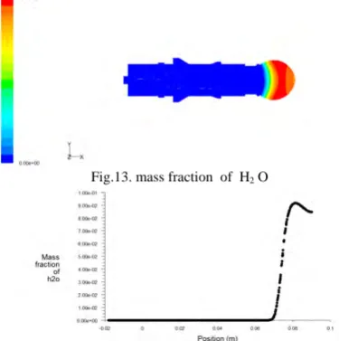
The figure 13, shown below indicates the contous of mass fraction of H2 O and the graph, figure 14, represents
the same with position. Initially the quantity is zero and when the combustion started the quantity of H2 O is
increasing and reaches a maximum of 0.076.
Fig.13. mass fraction of H2 O
Fig.14. mass fraction of H2 Owith position
3.1 Case-2.
In this case the inlet velocities of methane and air are considered as 0.2 m/s and 0.8m/s respectively. The following figure 15 represents the plane contours of temperature. From the figure we can say that the maximum temperature obtained is 2172k and then slightly decreases. The graph, figure16,shown below indicates the static temperature with position, and which shows the temperature increases and reaches a maximum of 2172k and then slightly decreases. The figure17represents the contours of temperature in the actual geometry.
Fig.16. static temperature with position
Fig.17. contours of temperatureof actual geometry
The following figure 18 indicates the contours of mass fraction of methane, which shows the mass fraction of unburned methane in the mantle is 0.079 which isless than compared to the previous case, and the graph, figure 19indicates the mass fraction of methane with position. From the graph we can see that the mass fraction of methane is decreasing and then slightly increasing, that means the unburned methane is very less.
Fig.18.contours of mass fraction of methane
Fig.19.mass fraction of methane with position
The following figure 20, shows the plane contours of mass fraction of oxygen and from the figure we can see that the masss fraction of oxygen is increasing from the inlet and at the mantle position the quantity of oxygen is very less. The graph, figure 21, shows the mass fraction of oxygen with position and from this graph we can understand the outer portion has less oxygen content.
Fig.21.mass fraction of oxygen with position
The figure 22, shown below indicates the contous of mass fraction of CO2and the graph, figure 23 represents
the same with position. Initially the quantity is zero and when the combustion started the quantity of CO2 is
increasing and reaches a maximum of 0.08 which is less than compared to the previous case .
Fig.22.contous of mass fraction of CO2
Fig.23.mass fraction of CO2 with position
The figure 24 shown below indicates the contous of mass fraction of H2 O and the graph, figure 25represents
the same with position. Initially the quantity is zero and when the combustion started the quantity of H2 O is
increasing and reaches a maximum of 0.066 which is also less than compared to the previous case.
Fig.24.contous of mass fraction of H2 O
3.2 Case-3.
In this case the inlet velocities of methane and air are considered as 0.3m/s and 0.8m/s respectively. The following figure26,represents the plane contours of temperature. From the figure we can say that the maximum temperature obtained is 2189k and then slightly decreases. The graph, figure27, shown below indicates the static temperature with position, and which shows the temperature increases and reaches a maximum of 2189k and then slightly decreases. The figure 28,represents the contours of temperature in the actual geometry.
Fig.26.plane contours of temperature
Fig.27.static temperature with position
Fig.28.contours of temperature in the actual geometry
Fig.30. mass fraction of methane with position
The above figure29,showing the contours of the mass fraction of methane and the graph figure 30,represents the mass fraction of methane with position. The distance from the inlet position the quantity of methane is decreasing and reaches a maximum of 0.088, which is greater than the previous case. The horizontal line in the x-axis represents the methane quantity is zero, this is due to the methane inlet is in annular shape.
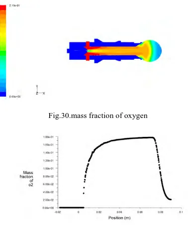
Fig.30.mass fraction of oxygen
Fig.31 Mass fraction of oxygen with position
The above figure 31,showing the contours of mass fraction of oxygen and the graph, figure 30,represents the mass fraction of oxygen with position which shows the combustion chamber has very less quantity of oxygen when the combustion is going on.
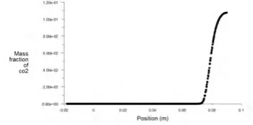
The figure 32 shown below indicates the contous of mass fraction of CO2and the graph, figure 33 represents the
same with position. Initially the quantity is zero and when the combustion started the quantity of CO2 is
increasing and reaches a maximum of 0.0587 which is less than compared to the previous case .
Fig. 32 contous of mass fraction of CO2
Fig. 33 Mass fraction of Co2 with position
The figure 34 shown below indicates the contours of mass fraction of H2 O and the graph, figure 35 represents
the same with position. Initially the quantity is zero and when the combustion started the quantity of H2 O is
increasing and reaches a maximum of 0.048 which is also less than compared to the previous case.
Fig. 34 Contours of mass fraction of H2 O
Fig. 35 Mass fraction of H2O with position
CONCLUSION
The present work simulates the flow and thermal characteristics of a typical biogas burner lamp flame. The optimum inlet velocities of air and methane are found to be 0.8 m/s and 0.2 m/s respectively. The maximum flame temperature obtained in this case is 2172 k, which is below the adiabatic flame temperature of methane. The main feature of this case is that the quantity of the unburned methane is very less compared to the other two cases.
REFERENCES
[1] R.K Pachauri, and A. Reisinger, Eds, “Climate Change 2007: Synthesis,” in Contribution of Working Groups I, II and III to the Fourth Assessment Report of the Intergovernmental Panel on Climate Change, Geneva, Switzerland: IPCC, 2007.
[2] A.F. Brancelli1, C. Mongiello2, C. Noviello1, F.R. Picchia2,Parametrical Analysis of a Biogas Fuel Combustion Process in a Chamber in Steady-State Condition, June 2003.
[3] Carlos Díaz-González1, Andrés-Amell Arrieta2 and José-Luis Suárez3,Comparison of Combustion Properties of Simulated Biogas and Methane, October 13, 2009.
[4] Saeed Jahangirian, Abraham Engeda, Proceedings of the IMECE2008 , 2008 ASME International Mechanical Engineering Congress and Exhibition October 31- November 6, 2008, Boston, Massachusetts, USA.
[5] AhamadSakhrieh, Effect of pressure and inlet velocity on the adiabatic flame temperature of a Methane–Air flame. Dept.of Mechanical enggPhiladelphia university, Jordan,jan 2010.
[6] Y. Lafay Æ B. Taupin Æ G. Martins Æ G.Cabot Æ B. Renou Æ A. Boukhalfa, Experimental study of biogas combustion using a gas turbine configuration, 29 April 2007.
[7] W. Blasiak, "Fuel Switch from fossil to 100% biomass Tangential fired PC boiler," in Proceedings of Power GEN Europe Milan, Italy, 2008.