Global Journal of Advanced Engineering Technologies and Sciences SUPPLIER SELECTION CRITERION IN UNCERTAIN PRODUCT COST: A DYNAMIC PROGRAMMING APPROACH Dhirendra Singh Parihar *1 , Manmohan Rahul 2

(1)

http://www.gjaets.com © Global Journal of Advance Engineering Technology and Sciences 78

Global Journal of Advanced Engineering Technologies and Sciences

SUPPLIER SELECTION CRITERION IN UNCERTAIN PRODUCT COST:

A DYNAMIC PROGRAMMING APPROACH

Dhirendra Singh Parihar

*1

, Manmohan Rahul

2 *1_{Ansal University,Gurgaon-122003 India.}

Ansal University,Gurgaon-122003 India.

Abstract

Supplier selection is very significant business problem for ensuring competitiveness on the market. A number of quantitative methods have been applied to solve this problem. In this paper a criterion to select a supplier is suggested in the cases where the product cost of the supplier varies with planned periods and is uncertain. The effect of variability on the optimal solution is illustrated with the help of a numerical example. The optimal cost for ten periods is estimated using forward dynamic programming approach. It is found that the optimal (minimum) cost increases with the variability in the product cost. One of the important finding of this study is that the supplier with less variability in product cost should be preferred.

Keywords:Supplier Selection, Inventory Lot Sizing, Dynamic Order Sizing, Optimal Ordering Cost.

Introduction

The problem with vendor selection and determining procurement quotas from selected vendor is the most important phase for a production company in the process of procurement of materials. Several studies addresses issues related to supplier selection. These studies have used different methods ranging from Analytic Hierarchy Process (AHP) (Nydic and Hill , 1992) and cost ratio method(Timmerman,1987) to total cost of ownership (ellram,1990;Gheidar Kheljani et al.,2009),linear programming(Ng,2008:Talluri and Narsimhan,2003), multi objective programming (Narsimhan et al.,2006) and DEA (Liu et al.,2000; Ramanathan ,2007;Weber,1996). Muralidharan et al., (2002) proposed an AHP based model in which nine criteria were used for ranking the suppliers. Furthermore, they take into account the opinions of experts from different departments such as purchasing and quality control in their model. Chan and Chan (2010) developed an AHP based model for supplier evaluation and selection as well as Muralidharan (2002) with a case in fashion industry.

In today’s business environment, companies need to operate in a efficient and effective manner in order to survive. The purchasing management and inventory management are important decision making areas. Mathematical programming methods are important tools to find favorable decisions. Applications of inventory control and management have been extensibly studied in the related literature. Many researchers have studied the problem to consider the most appropriate suppliers ,a and to determine the optimal lot size for each product in each planning period to minimize the total inventory holding cost. Brahim et al. (2008 ) presented a comprehensive review of lot sizing problem in the case where demand of the product varies over different time periods. Heady and Zhu(1994) improved the solution procedure proposed by Wanger and Whitin (1958). The supplier selection problem without inventory consideration was studied by Current and Weber (1994).

The problem with multiple Suppliers with inventory considerations is studied by various workers. Aissaoui et al.(2007) developed a well known economic order quantity model to discuss the problem of multi suppliers. The lot sizing with single product with discount rate was solved by Tempelmeir (2002) with a heuristic method. Basnet and Leung (2005) considered the supplier selection and order lot sizing problem with multiple products each with different deterministic demand. M.M.Moqri et al. (2011) discussed a multi period integrated supplier selection and order lot sizing problem where a single buyer plans to purchase a single product in multiple periods from several suppliers. They developed a mathematical programming model and proposed a forward dynamic programming approach to obtain the optimal solution.

(2)

of variability on optimal solution is illustrated by taking a numerical example. The various optimal solutions are obtained for different values of standard deviation. Different replicates of the solution are calculated and the average value of optimal solution is obtained.

Methodology

We assume that:

i) Products are shipped directly from supplier to the buyer (i.e., there is no intermediate distributor). ii) Only one product is considered.

iii) Supplier’s capacity is unlimited.

iv) Buyer’s demand is deterministic and is known in advance. v) Order lead time is zero.

vi) No product shortage is permitted. vii) The planning horizon is finite.

viii)The lot size does not exceed the demand of the period.

The functional equation (Bellman, 1957, Karlin, 1955) representing the minimum cost policy for periods t through N, is given as:

𝒇𝒕(𝑰) =

𝒎𝒊𝒏 𝒙𝒕 ≥ 𝟎

𝒊𝒇 𝒙𝒕≥ 𝒅𝒕

[𝒊𝒕−𝟏𝑰 + 𝜹(𝒙𝒕)𝑺𝒕+ 𝒇𝒕−𝟏(𝑰 + 𝒙𝒕− 𝒅𝒕)] (𝟏)

where

𝛿(𝑥𝑡) = {_{1 𝑖𝑓 𝑥}0 𝑖𝑓𝑥𝑡= 0 𝑡> 0

I=the inventory entering a period I0 =initial inventory

dt= demand in period t

it=inventory holding cost per item

St=setup(ordering) cost

xt= amount ordered (or manufactured )

t=1, 2 , 3 ………..,N

The alternate formulation to equation (1) proposed by Wanger and whitin (2004) is as follows:

𝑭(𝒕) = 𝐦𝐢𝐧

[ 𝒎𝒊𝒏

𝟏 ≤ 𝒋 < 𝒕 [𝒔𝒋+∑ ∑ 𝒊𝒉𝒅𝒌+ 𝑭(𝒋 − 𝟏) 𝒕

𝒌=𝒉+𝟏 𝒕−𝟏

𝒉=𝒋

]

, 𝒔𝒕+ 𝑭(𝒕 − 𝟏) ]

(𝟐)

where F(1) = S1 and F(0) =0

The equation (2) states that the minimum cost for first t periods comprise a setup(ordering) cost in period j ,plus charges for filling demand 𝑑𝑘, 𝑘 = 𝑗 + 1, … , 𝑡 by carrying inventory from period j, plus the cost of adopting an optimal policy in period 1 through j-1 taken by themselves. In general if the product price varies in different periods, we have

𝑭(𝒕) = 𝐦𝐢𝐧

[ 𝒎𝒊𝒏

𝟏 ≤ 𝒋 < 𝒕 [𝒔𝒋+∑ ∑ 𝒊𝒉𝒅𝒌+ 𝒑𝒋(∑ 𝒅𝒋 𝒕

𝒊=𝒋

) + 𝑭(𝒋 − 𝟏)

𝒕

𝒌=𝒉+𝟏 𝒕−𝟏

𝒉=𝒋

]

, 𝒔𝒕+ 𝑭(𝒕 − 𝟏) ]

(𝟑)

(3)

Their algorithm for calculation is given below in tabular form (Table 1).

Table 1: Procedure to calculate minimum ordering cost for N periods

Periods 1 2 3 - N

1 1 (1)2 (1,2)3 - (1,2,…..,N-1)N

2 12 (1)23 - (1,2,…..,N-2)N-1,N

3 123 - (1,2,…N-3)N-2,N-1,N

. . .

N

Minimum(Rs.) (1) (1,2) (1,2,3) - (1,2,3,………N)

Row 1 and column 1 of the table represents number of order periods and minimum ordering cost for a particular order respectively. The tabular calculations shown in table 1 are as follows:

a) In the second column of Table 1,the order quantity must be equal to the demand of period 1, therefore ,the value of second and the last row of the column 2 is equal to the sum of the ordering and purchasing cost to meet the demand of the product in period 1 and is denoted by (1).

b) The second row of third column is a policy in which an order is placed in the second period; therefore, in both periods 1 and 2 , an order is placed and the cost of the policy is denoted by (1, 2).

c) The third row of the third column represents a policy in which an order equal to the demands of both periods 1 and 2 is placed in period 1. The cost of this policy is denoted by 12. The minimum cost for period 2 is given in the last row of third column and is denoted by (12). This includes the holding cost inventory which is carried from period 1 to 2.

d) For the column 4, there are three ordering options:

(i) an order is placed in period 3 is equal to the demand in this period and demands of periods 1 and 2 are ordered optimally. The total cost of this policy is denoted by (1, 2)3.

(ii) an order is placed in period 2 to satisfied demands of 2 and 3 and demand of period 1 is ordered optimally. The total cost of this policy is denoted by (1)23.

(iii)an order s placed in period 1 to satisfied all the demands of periods 1 though 3. The total cost of this policy is denoted by 123. The minimum cost for period 3 is denoted by (123).

The similar procedure is adopted for the rest of periods.

The uncertain product cost is assumed to follow the normal probability distribution. The optimal solution for various variations (standard deviations) in the product cost is calculated. The average of various replicates of the optimal solution is obtained to represent the optimal solution.

Results And Discussion

The effect of uncertainty in product cost on optimal solution is illustrated with the help of the following numerical example:

The product demand per period =200. The mean cost over the periods =Rs.2. The inventory holding cost per product =Rs.1. The ordering cost = Rs. 400.

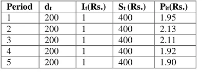
The product cost is uncertain and follow the normal probability distribution with mean= 𝜇 and standard deviation =𝜎. Following the procedure described in methodology the optimal cost for ten periods have been calculated. The parameters of numerical example are given in Table 2.

Table 2: Parameters of numerical example (μ = Rs.2, σ =10)

Period dt It(Rs.) St (Rs.) Pit(Rs.)

1 200 1 400 1.95

2 200 1 400 2.13

3 200 1 400 2.11

4 200 1 400 1.92

(4)

6 200 1 400 2.05

7 200 1 400 1.99

8 200 1 400 1.89

9 200 1 400 1-83

10 200 1 400 1.96

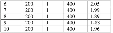
The minimum cost for each period for the numerical example given in Table 2 is found using forward dynamic programming approach described in methodology, and is shown in Table 3.

Table 3. Optimal (minimum) cost (Rs.) solution (μ=2, σ=10)

Periods 1 2 3 4 5 6 7 8 9 10

1 804 1619 2244 3048 3622 4400 4406 4770 5534 6268

2 1408 2388 2880 3684 3822 4978 4928 5734 6098

3 2212 3280 3716 3684 4906 5756 5650 6498

4 3216 4372 4652 5556 5848 6734 6572

5 4420 5664 5988 6792 6990 7912

6 5224 7156 7424 8228 8332

7 7428 8848 9060 9864

8 9232 10740 10896

9 11236 12832

10 13440

Minimum(Rs.) 804 1408 2212 2880 3622 3684 4406 4770 5534 6098

The two replicates of the solution given in table 3 are found and are given in table 4 and table 5 respectively. The average of the optimal (minimum) cost for tenth period of from three replicates is given in table 6.

Table 4. Replicate-2 of the solution presented in Table 3

Period 1 2 3 4 5 6 7 8 9 10

1 754 1594 2164 2854 3694 4214 4214 4496 5356 6204

2 1308 2234 2820 3446 3894 4782 4782 5378 6016

3 2062 3074 3676 3446 5242 5550 5550 6060

4 3016 4114 4732 5230 6316 6518 6518

5 4170 5354 5988 6422 7590 7686

6 5524 6794 7444 7814 9064

7 7078 8434 9100 9406

8 8832 10274 10956

9 10786 12314

10 12940

Minimum(Rs.) 754 1308 2062 2820 3446 3446 4214 4496 5356 6016

Table 5. Replicate-3 of the solution presented in Table 3

Peri0d 1 2 3 4 5 6 7 8 9 10

1 836 1642 2298 3040 3744 4402 4458 4886 5664 6444

2 1472 2248 2924 3632 3944 4972 5084 5914 6250

3 2308 3054 3750 3632 5184 5742 5910 6742

4 3344 4060 4776 5416 6204 6712 6936

5 4580 5266 6002 6608 7424 7882

6 6016 6672 7428 8000 8844

7 7652 8278 9054 9592

8 9488 10084 10880

9 11524 12090

(5)

Minimum(Rs.) 836 1472 2248 2924 3632 3632 4458 4886 5668 6250

Table 6. Average minimum cost obtained from replicates of the solution for tenth period

Replicate 1 2 3

Minimum cost(Rs.) 6098 6016 6350

Average=Rs.6121

In the next experiment the optimal solution is obtained with an increase in variability in product cost. The parameters of numerical example considered are same as previous numerical example except the standard deviation. The product cost distribution in ten periods is obtained using normal probability distribution with μ=2 and σ=20. Thus the columns of numerical example (Table 2) remain same except last column. The last column represents the large variability in product cost as compared to Table 2. The modified numerical example with σ=20 is not shown. The optimal cost for this experiment is shown in Table 7.

Table 7. Minimum cost (Rs.), μ =2, σ =20, dt =200, It =1 (Replicate-1)

Period 1 2 3 4 5 6 7 8 9 10

1 886 1714 2522 2978 3824 4210 4306 4768 5518 6280

2 1572 2342 3272 3414 4024 4806 4998 5830 6068

3 2458 3170 4222 3414 4932 5602 5890 6692

4 3544 4198 5372 4886 5786 6598 6982

5 4830 5426 6722 5922 6840 7794

6 6316 6854 8272 7158 8094

7 8002 8482 10022 8594

8 9888 10310 11972

9 11974 12338

10 14260

Minimum(Rs.) 886 1572 2342 3170 3414 3414 4306 4768 5518 6068

Table 8. Replicate-2 of the solution given in Table 7.

Period 1 2 3 4 5 6 7 8 9 10

1 728 1500 1930 2680 3266 3804 4060 4454 5384 6192

2 1256 2072 2404 3230 3466 4330 4690 5448 6114

3 1984 2844 3078 3230 4790 5056 5520 6242

4 2912 3816 3952 4930 5852 5982 6550

5 4040 4988 5026 6080 7114 7108

6 5368 6360 6300 7430 8576

7 6896 7932 7774 8980

8 8624 9704 9448

9 10552 11676

10 12680

Minimum(Rs.) 728 1256 1930 2404 3078 3230 4060 4454 5384 6114

Period 1 2 3 4 5 6 7 8 89 10

1 924 1770 2498 3082 3958 4370 4432 4904 5730 6604

2 1648 2416 3148 3548 4158 4992 5116 5976 6356

3 2572 3262 3998 3548 5378 5814 6000 6848

4 3696 4308 5048 5080 6388 6836 7084

5 5020 5554 629 6146 7598 8058

6 6544 7000 7748 7412 9008

7 8268 8646 9398 8878

8 10192 10492 11248

9 12316 12538

10 14604

(6)

The replicates of the solution presented in Table 7 are given in Tables 8 and 9 respectively.

The average minimum cost for tenth period is given in Table 10.

Table 10.The average minimum cost for period -10.

Replicates 1 2 3

Minimum cost(Rs.) 6068 6114 6356

Average = (608+6114+6356) / 3 = 6179

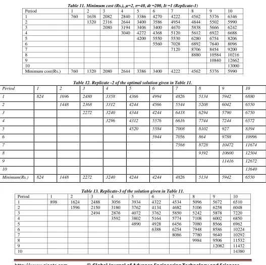
The third experiment is carried out with further increasing variability in the product cost. In this case the mean cost (μ) is same (Rs. = 2) but the standard deviation (σ) is taken equal to 40. All other parameters of the numerical example are same. The optimal cost solution with these parameters is given in Table 11.

Table 11. Minimum cost (Rs.), μ=2, σ=40, dt =200, It =1 (Replicate-1)

Period 1 2 3 4 5 6 7 8 9 10

1 760 1638 2082 2840 3386 4270 4222 4562 5376 6346

2 1320 2316 2644 3400 3586 4954 4844 5502 5990

3 2080 3194 3406 3400 4670 5838 5666 6242

4 3040 4272 4368 5120 5612 6922 6688

5 4200 5550 5530 6280 6754 8206

6 5560 7028 6892 7640 8096

7 7120 8706 8454 9200

8 8880 10584 10216

9 10840 12662

10 13000

Minimum cost(Rs.) 760 1320 2080 2644 3386 3400 4222 4562 5376 5990

Table 12. Replicate -2 of the optimal solution given in Table 11.

Period 1 2 3 4 5 6 7 8 9 10

1 824 1696 2480 3358 4366 4994 4826 5134 5942 6880

2 1448 2368 3312 4244 4566 5544 5208 6042 6550

3 2272 3240 4344 4244 6418 6294 5790 6750

4 3296 4312 5576 6616 7744 7244 6572

5 4520 5584 7008 8102 927 8394

6 5944 7056 864 9788 10996

7 7568 8728 10472 11674

8 9392 10600 12504

9 11416 12672

10 13640

Minimum(Rs.) 824 1448 2272 3240 4244 4244 4826 5134 5942 6550

Period 1 2 3 4 5 6 7 8 9 10

1 898 1624 2488 3056 3934 4322 4534 5096 5672 6510

2 1596 2150 3180 3762 4134 4682 5106 6258 6048

3 2494 2876 4072 3762 5850 5242 5878 7220

4 3592 3802 5164 5774 7108 6002 6850

5 4890 4928 6456 7080 8566 6962

6 6388 6254 7948 8586 10224

7 8086 7780 9640 10292

8 9984 9506 11532

9 12082 11432

(7)

Minimum(Rs.) 898 1596 2150 2876 3762 3762 4534 5096 5672 6048

The replicates of the solution given in Table 11 are given in Tables 12 and 13. The average optimal solution in this case is given in table 14.

Table 14. The average Minimum cost (Rs.) from replicates.

Replicates 1 2 3

Minimum cost 5990 6550 6048

Average = (5990+6550+6048) / 3 = 6196

The results obtained from the numerical example illustrate that the uncertainty in product cost affects the optimal solution for the minimum cost. We found that as the variability in the product cost increases the minimum cost increases . The average optimal cost calculated from three experiments for last period for different values standard deviation is shown in Table 15.

Table 15. Variation of minimum cost for tenth period with variation in standard deviation.

σ 10 20 40

Average minimum cost(Rs.) 6121 6179 6196

The above Table shows that as the variation in product cost increases the minimum cost increase.

Conclusion

The forward dynamic programming approach is used to study the effect of uncertainty in the cost of the supplier product on the optimal cost solution. The cost of the product is different in each period and is uncertain. The cost is assumed to follow the Normal probability distribution .The effect of the uncertainty in the product cost on the optimal solution is illustrated by taking a numerical example.. The optimal solution is found for various values of the standard deviation of the product cost . It is found that as the standard deviation of product cost increases the optimal (minimum) cost for each period increases. One of the important conclusions of this study is that in case of uncertain variability in product cost, a supplier should be selected with less variability in product cost.

References

1. Aissaoui, N., Haouari,M. and Hassini,E.,2007. Supplier selection and order lot sizing modeling : A review. Computers and Operations Research, 34,3515-3540.

2. Basnet, C. and Leung,T.M.Y.,2005. Inventory lot sizing with supplier selection. Computers and Operations Research,32,1-14.

3. Brahimi,N. ,Daugere-Press,S. ,Najid,A.,2006. Single item lot sizing problem. European journal of operational Research,168,1-6.

4. Chan,F.T.S., and Chan,H.K.,2010.An AHP model for selection of suppliers in the fast changing fashion market. International Journal of Advanced Manufacturing Technology,51(91),1195-1207.

5. Current,J. and Weber,C.,1994. Application of facility location modeling constructs to vendor selection problems.European Journal of Operational Research,76,387-392.

6. Dai,T. and Qi,X. ,2007. An acquisition policy for a multi supplier system with a finite time horizon. Computers and Operations Research,34,2758-2733.

7. Ellram ,L.M.,1990. The supplier selection decision in strategic partnership. Journal of Purchasing and Material Management,26(4),8-14.

8. GheidarKheljani,J., Ghodsypour,S. and O’Brein,C.,2009. Optimizing whole supply chain benefit through supplier selection.International Journal of Production Economics,121(2),482-493.

9. Heady,R.B. and Zhu ,Z.,1994. An improved implementation of the Wanger-Whithin algorithm . Production and Operation Management,3,55-63.

10. Lin,J.,Ding , F.Y.and LK,V.,2000.Using Data Development Analysis to compare suppliers for supplier selection and performance improvement.Supply chain Managemnt ,5(3),143-150.

11. Moqri,M.M., and Moshref Javedi ,M. and Yazdian,S.A.,2011.Supplier selection and lot sizing using dynamic programming. International Journal of Industrial Engineering Computations,2,319-328.

(8)

13. Ng ,W.,2008. An efficient and simple model for multiple criteria supplier selection problem . European Journal of Operation Research ,186(3),1059-1067.

14. Nydick,R.L. and Hill,R.P.,1992.Using the analytic hierarchy process to structure the vendor selection process. International journal of purchasing and material management,28(2),31-36.

15. Ramanathan,R.,2007. Supplier selection problem : Integrating D.E.A. with the approaches of total cost of ownership and A.H.P. Supply chain Management: An international Journal,12(4),258-261.

16. Talluri,S. and Narashimashimahan,R. ,2003. Vendor evaluation with performance variability: A max-Mn approach. European Journal of Operation Research ,146(3),543-552.

17. Tempelmeier,H.2002. A simple heuristic for dynamic order sizing and supplier selection with time varying data. Production and Operations Management ,11,499-515.

18. Timmerman,E.,1987. A n approach to vendor performance evaluation. Engineering Management Review,Ieee,15(3),14-20.