Multiresponse model based design parameters optimization: engineering approach

Multiresponse model based design parameters

optimization: engineering approach

S.A. Popov

1,

*, A.M. Abramov

2

1 _{Department Engineering Technology, Yaroslav-the-Wise State Novgorod University (NovSU),} ul. B.S. Peterburgskaya 41, Veliky Novgorod, 173003 Russia

2 _{Department Engineering Technology, Yaroslav-the-Wise State Novgorod University (NovSU),} ul. B.S. Peterburgskaya 41, Veliky Novgorod, 173003 Russia

Abstract

A practical algorithm of determination of the set of Pareto optimal output parameters and a solution of the reverse optimization problem have been proposed. Basics of building and usage of multiresponse model are presented, which allows to perform multicriteria optimization optimization for different design and manufacturing situations.

Keywords: Pareto optimal parameters, reverse optimization, multi-criteria optimization, multiresponse model. Received on 02 June 2017, accepted on 12 July 2017, published on 14 July 2017

Copyright © 2017S.A. Popov, A.M. Abramov, licensed to EAI. This is an open access article distributed under the terms of the Creative Commons Attribution licence (http://creativecommons.org/licenses/by/3.0/), which permits unlimited use, distribution and reproduction in any medium so long as the original work is properly cited.

doi: 10.4108/eai.14-7-2017.152891

*_{S.A. Popov. Email:[email protected]}

1. Introduction

Well-founded definition of regions of admissible values of the vector of input (independent) constructive or technological parameters X = x1,x2,…xkT , allows to exclude non-optimal solutions at the early stages of design or in the technological process. To solve this problem, it is necessary to build a model of the dependence of the vector of output parameters Y=

y1,y2,…ymT from the input parameters and on its basis to solve the problem of determining the optimum values of the output parameters taking into account the available technological (constructive) constraints [1].

Then, for the obtained optimal values of the output parameters, it is necessary to determine the corresponding values of the input parameters (the inverse optimization problem).

2. Definition of the regions of admissible

values of output parameters

The region N of changing of the input parameters is determined by the physical factors and is usually given by a system of inequalities in the form of xi1  xi

xi2,i1,k..The region M of admissible values of output parameters (parameters-acceptance criteria) Y=

y1,y2,…ymT is given by the normative values of these parameters in the form of a system of inequalities yj1 yj

yj2. j1,m. Vector X= x1,x2,…xk in the space of the input technological parameters determines the point in the space of the parameters- acceptance criteria corresponding to the given article.

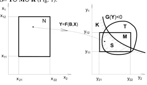
If the transformation XY is known in the form of a multiresponse function Y = F(X,B), where F(X,B) – multiresponse function, which is determined experimentally, and B is a coefficient vector, then for a given point X in the space of input parameters it is possible to determine the corresponding point Y in the space of output parameters. Thus, a k-dimensional region N (km) is represented into the space of output parameters in the form of a m-dimensional region T.

There are, also, functional limitations, determined by the principles of operation of the designed equipment or technological process.

These constraints are represented as a system of inequalities G(Y) 0 and they define the region K for which these constraints are satisfied [2].

If the point X corresponds to a point Y inside the region of nondefective items M (YM), then this product meets the requirements of the technical specifications for these parameters Taking into account functional limitations, the desired region S of output parameters is determined by the intersection of the regions T, M, K, i.e. S= T M K (Fig. 1).

Fig. 1. Determination of the region S of admissible values of output parameters

3. Solution of the inverse optimization

problem with incontrollable input

parameters

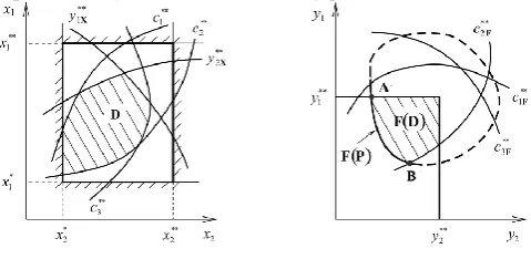
The task of determining the admissible input parameters is the determination of such region of input parameters which ensures the belonging of the given article to the class of nondefective ones, which is the content of the problem of reverse optimization. If the image L of the region S is defined in the space of input parameters, then it is possible to specify the technological parameters X L, ensuring certainly nondefective articles (Fig. 2). To specify independent intervals of the admissible values of technological parameters in the region L, it is necessary to inscribe the k-dimensional parallelepiped R in accordance with the criterion of optimality.

If the input parameters are uncontrollable and have scatted values (Fig. 2), then the percentage of yield is used as a criterion for the optimality of the intervals of admissible values.

Fig. 2. Obtaining independent intervals of admissible values for input technological parameters

In this case, the optimal region R is constructed on the basis of the joint probability density function of the input parameters (xi). The criterion of optimality D for determining the intervals of admissible values is the yield of nondefective articles by technological parameters in the form





k

x

x x

x x

x

k dxdx dx x

x x

k

k

 

 1 2 1 2

12

11 22

21 2

1

, , ,

D

  

 , (1)

where 



x1,x2,,x_k



is the joint probability density function of technological parameters.

The construction of the region R in accordance with the criterion of optimality (1) is performed by the method of statistical tests.

4. Construction of a multiresponse

model and its use for determining input

parameters

The XY transformation is represented as a multiresponse model

Y = F(X,B),

(2) where F(X,B)= f1(X,B), f2(X,B), …, fm(X,B)T is m -dimensional vector of the functions, Y= y1,y2,…ymT are admittance/reject criterion (responses), X= x1,x2,…xk

T are independent variables, B= b1,b2,…blT is l -dimensional vector of coefficients whose exact values are determined from the experimental data.

In the general case, the calculation of the estimates of the coefficients of the model (2) is carried out using an iterative procedure [3]



















 _{ } n _

j

s j j s j s

s

1

1 1

,

,B V Y FX B

X P K B

B _E , (3)

where matrix V_E is covariance matrix of observation errors and

 



 







   

 

  

   

B B X B

B X B

B X X

 

 

1

1

T 1







    

   



n

j

j j S P X X

P

K E , (4)

where S_E is covariance matrix estimate V_E.

The constructed model can be used to solve the inverse problem, that is, to estimate the values of the input parameters for given values of the output parameters. When the type of the model (2) is selected and the estimates of its coefficients (3) are calculated, the calculation of the estimates of the input values of the parameters is performed by the formula



B,Y



F

X 1 , (5)

where F1

 

 is the function inverse to the function F

 

 ,

Y is the vector of the output parameters.

Expanding expression (2) in terms of independent variables in a Taylor series, we obtain



B,X



X

Y 

 Ω , (6)

where













   

 

  

   

X X B, X

X B, X

X

B, f_m

, f

, f

ΩT 1 2 _

.

Then, in the case of the equality of the number of independent and dependent variables, the solution of the nonlinear problem (6) can be obtained by the following iterative procedure

 

s s

s1_{  Ω}1_Δ

X

X , (7)

where

s

is iteration number, ΔYF



B,X



.

The covariance matrix V_X of the estimates X is derived from expression (6) and is equal to

VXΩ1PT



B,X



VBP



B,X



 

Ω1T. (8)

If the number of input parameters k is greater than the number of output parameters m, then for solving the equation (5) it is necessary to specify (k-m) input parameters, and the remaining m input parameters are determined according to equation (7)

When constructing the model (2), it is necessary to perform:

(i) analysis of the covariance matrix of observation errors;

(ii) the choice and justification of the model;

(iii) checking the significance of coefficient estimates; (iv) checking the adequacy of the model.

4. Approximation of the admissible set

of input parameters

As a result of analyzing the matrix W, the region of admissible values of the input parameters is presented in a discrete form and its boundaries are not defined analytically. Often in practice, this form of the region of permissible values leads to problems when trying to analyze it and use it for decision making. For example, when a vector of input parameters is set on the boundary

of an admissible region, it is not clear whether it enters the region of admissible values.

To solve the approximation problem, the form of the region of admissible values should be approximated by some analytic surface. This convolution of the region of admissible values greatly simplifies its use. For example, it allows to easily set the desired input parameters within this region. To identify the shape of a admissible region, it is possible to construct it in the form of a separating surface that includes all (or at least the majority) values of the input parameters related to the admissible region and does not include parameters that are not within the admissible region.

In these circumstances, it is proposed to use the method of least squares to construct a separating surface [5]. ]. In accordance with this method, estimates of the coefficients A of the separating surface g



X,A



0 are calculated so that they provide a minimum of the sum of squares of deviations in the form

















   

 

 







 

n

i

i i n

i

i

i y y

1

2 1

2

, g min ,

gX A X A

B , (9)

where g



X,A



is separating function, X



x₁,x₂,,x_r



T

is vector of parameters, A



a₁,a₂,,a_l



T is vector of coefficients, y is the attribute of the point of the admissible region (for example, y = 1 if the parameter enters the admissible region, and y = -1 otherwise), n is the sample size.

However, with this approach, the contribution to the sum of the deviations (9) will be given by parameters with large values of the function g



X,A



, which leads to significant recognition errors, especially in the complex form of the separating function, which is typical for technical applications.

We assume that for each parameter there is a probability of belonging to an admissible region q1 and

the probability does not belong to this region q₂ (q1q2 1). Experimentally belonging to the admissible region (y1) is determined from the matrix W (the parameters enter the matrix W).

This gives an estimate y of the value of the membership function q

 

X q₁q₂ as a function of the magnitude of the parameter vector.

As a result of the construction of an admissible region for n items, the estimation of the membership vector





T

2 1,y , ,yn

y 



Y is determined. Approximation of the

dependence of the magnitude q on the values of the parameters can be presented in the form [6]:



X,B



sign



f



X,A







1 exp



f



X,A







q    , (10)

where f



X,A



is some approximation of function



X,A



g .

away from the separating surface. The separating surface is determined by the equation



,



0

gXA  . (11)

Inthis case, the calculation of the coefficient estimates in expression (11) by the least squares method is performed using the following iterative procedure [6]:

















 _{ } n _

i

i i s i s

s

y

1 1

,

,A qX A

X P V A

A _A , (12)

where s is iteration number and

















A A X A X A

X A

X P

  

signf( , )exp f , f( , )

, .

For a complete quadratic function with three parameters,

for example, one can obtain



₂



T

3 3 1 2 1 3 2

1, , , , , ,

, 1 ) , f(

x x x x x x x

x 

  

A A X

.

Covariance matrix for estimating coefficients A is calculated by the formula



 



1

1

T 2

, ,



 

 

  



n

i

i i

e PX AP X A

VA  , (13)

where _e2 is variance of class recognition error.

As an estimate of the variance in the recognition of classes, we used the estimate of the variance of the model's adequacy error, calculated by the formula:













 

 n

i

i i

e y

l n s

1

2

2 1 _{qX ,A , (14)}

where l is number of coefficients in the model (11). The diagonal elements of the matrix V_B (13) represent the variances of the estimates of the corresponding coefficients, which makes it possible to calculate their t -statistics and, therefore, to verify the significance of the coefficient estimates.

The lower bound of the one-sided confidence interval for the separating function that ensures the probability of recognizing the first class of at least P% is defined as:

q



X,A

 

qX,A



t_P,fs_e, (15) where t_P is Student's quantile for confidence probability

P and number of degrees of freedom f, A is coefficient estimator vector.

Then the separating surface is defined by the expression



,



0

qXA t_P,fs_e . (16) By changing confidence probability P, one can achieve such a "compression" of region g



X,A



so that it does not include points that do not belong to the admissible region D. In this case, the resulting surface will be inscribed into the region D with some "reserve".

To calculate vector of estimates of the coefficients of separating function A in accordance with iteration procedure (12), a computer program has been developed. A two-dimensional illustration of the construction of approximating surface for three parameters is shown in Fig.3.

Fig. 3. Approximation of a two-parameter region of admissible values D by an inscribed ellipse DE with

a given confidence probability

5. Construction of a discrete

Pareto-optimal set

The Pareto-optimal set will be constructed on the basis of the matrix E, which determines the admissible set of input parameters D. The search for Pareto-optimal points is performed among the rows of the matrix W in accordance with the following conditions

The point X_i (XiD) is Pareto optimal if there is no

such point XD that f_

 

X f_

 

X_i for all v1,mk

and at least for one v exists f_

 

X f_

 

X_i . A set PD

is called Pareto-optimal if it consists of all Pareto optimal points. Based on the analysis of the Pareto-optimal set, the decision-maker determines the most preferable option

.

0

X

Pareto set is important for multicriterion optimization tasks, because, firstly, it is easier for designer to analyze it than the entire admissible set, secondly, whatever system of preferences designer used when comparing different vectors from the admissible region, the optimal vector always belongs to the Pareto set. It is known [1] that if admissible set D is closed and criteria f_

 

X are continuous, then Pareto set is not empty. This means that in any project task, we must determine the set of Pareto-optimal solutions.

The construction of Pareto-optimal set begins after obtaining admissible set D in the space of input parameters in the form of a matrix W. The first r columns of this matrix form discrete admissible set D in the space of input parameters containing s points.

parameters- acceptance criteria and for which technical limitations are not specified, but which are desirable to be optimized.

For each point X_i all local criteria are calculated

 

i v X

f , v1,mk. Thus, for each test point, a line is obtained in test table W, which has dimensions







n mk



in the form of:

 

 

 

 

 

 

_    

       

 

 

 

f

f

f f

f f

, 1

,

2 , 2 2

1 , 2

1 , 1 1

1 , 1

1 2 21

1 11

n k m n n

m n

k m m

k m m

nr n

r r

x x

x x

x x

X X

X X

X X

W

   

 

   

 

, (17)

where n is number of test points, m is number of parameters-acceptance criteria, k is number of controlled output parameters that are not constrained.

By checking the conditions for a point to belong to Pareto-optimal set for all points of the matrix W (17), only the Pareto-optimal points remain in this table.

Consider simplified illustration of constructing Pareto-optimal solution set (the criteria should be minimized). In Fig. 4 Pareto-optimal set in the space of criteria is represented by solid line confined by points A and B.

Fig. 4. The Pareto set F

 

P obtained with functional and criterial constraints

Conclusion

The proposed engineering method for constructing an admissible set of parameters allows one to obtain an admissible set in an analytical form, which makes it possible to provide an admissible probability of an error of its construction. The Pareto-optimal set is constructed in discrete form with a specified accuracy. The optimization procedure is based on a multiresponse model, the construction of which is the first stage of multi-criteria optimization.

References

[1] Sobol, I. and , Statnikov, R. (2006) The choice of optimal parameters in problems with many criteria. М.: Drofa. [2] Fyodorov, V. (1971) Theory of optimal experiment. М.:

Nauka.

[3] Podinovsky, V. and Nogin, V. (2007) Pareto-optimal solutions of multicriteria problems. М.: Fizmatlit. [4] Fletcher, R. (1980) Practical Methods of Optimization

N.Y.: John Wiley and Sons.

[5] Popov,S (2010) Construction and use of a separating surface for determining the composition of a multicomponent mixture. Factory Laboratory. Diagnosis of materials vol.: 4, p. 40-42