A kernel based true online Sarsa(
λ
) for continuous space
control problems
Fei Zhu1,2, Haijun Zhu1, Yuchen Fu3, Donghuo Chen1, and Xiaoke Zhou4
1 School of Computer Science and Technology, Soochow University
Shizi Street No.1 158 box, 215006, Suzhou, Jiangsu, China [email protected], [email protected], [email protected] 2
Provincial Key Laboratory for Computer Information Processing Technology, Soochow University
Shizi Street No.1 158 box, 215006, Suzhou, Jiangsu, China 3
School of Computer Science and Engineering, Changshu Institute of Technology [email protected]
4
University of Basque Country, Spanish [email protected]
Abstract. Reinforcement learning is an efficient learning method for the control problem by interacting with the environment to get an optimal policy. However, it also faces challenges such as low convergence accuracy and slow convergence. Moreover, conventional reinforcement learning algorithms could hardly solve con-tinuous control problems. The kernel-based method can accelerate convergence speed and improve convergence accuracy; and the policy gradient method is a good way to deal with continuous space problems. We proposed a Sarsa(λ) version of true online time difference algorithm, named True Online Sarsa(λ)(TOSarsa(λ)), on the basis of the clustering-based sample specification method and selective kernel-based value function. The TOSarsa(λ) algorithm has a consistent result with both the forward view and the backward view which ensures to get an optimal policy in less time. Afterwards we also combined TOSarsa(λ) with heuristic dynamic pro-gramming. The experiments showed our proposed algorithm worked well in dealing with continuous control problem.
Keywords: reinforcement learning, kernel method, true online, policy gradient, Sarsa(λ).
1.
Introduction
In many practical applications, the tasks that have to be solved are often with continu-ous space problems, where both the state space and the action space are continucontinu-ous. Most common methods of solving continuous space problems include value function methods [13] and policy search methods [2]. The policy gradient method [16] is a typical policy search algorithm which updates policy parameters in the direction of maximal long-term cumulative reward or the average reward and gets optimal policy distribution. The policy gradient method has two parts: policy evaluation and policy improvement. Reinforcement learning has many fundamental algorithms for policy evaluation is concerned, such as value iteration, policy iteration, Monte Carlo and the time difference method (TD) [9] where the time difference method is an efficient strategy evaluation algorithm. Both the value function in the policy evaluation and the policy function in the policy improvement require function approximation [3]. The policy evaluation and policy improvement of the policy gradient method can be further summarized as the value function approximation and the policy function approximation. In reinforcement learning algorithms, the approx-imation of the function can be divided into parametric function approxapprox-imation where the approximator and the number of parameters need to be predefined, and nonparametric function approximation where the approximator and the number of parameters are de-termined by samples. So nonparametric function approximation has high flexibility, and has better generalization performance. Gaussian function approximation and kernel-based method are nonparametric function approximation methods.
Although conventional reinforcement learning algorithms can deal with online learn-ing problems, most of them have low convergence accuracy and slow convergence speed. The kernel based method is nonparametric function approximation method, and its ap-proximation value function or strategy can alleviate the above problem of reinforcement learning. The policy gradient is an efficient way to deal with continuous space problems. In this paper, we propose an online algorithm that is based on kernel-based policy gradi-ent method to solve continuous space problem. In the Section 2, we introduce the related work, including Markov decision process, reinforcement learning, and policy gradient; in the Section 3, we state how forward view matches backward view; in the Section 4, we introduce a true online time difference algorithm, named TOSarsa(λ); in the Section 5, we combine TOSarsa(λ) with heuristic dynamic programming.
2.
Related Work
2.1. Markov Decision Process
Markov Decision Process (MDP) [5] is one of the most influential concepts in reinforce-ment learning. Markovian property refers that the developreinforce-ment of a random process has nothing to do with the history of observation and is only determined by the current state. The state transition probability with a Markovian stochastic process [12] is called the Markov process. By Markov process, a decision is made in accordance with the current state and the action set, affecting the next state of the system, and the successive decision will be determined with the new state.
Normally a Markov Decision Process model can be represented by a tupleM=<S,
A,f,r>, where:
Ais the action space, andat∈Adenotes the action taken by the agent at timet;
f:S ×A −→[0,1] is the state transfer function, andf is usually formalized as the probability of the agent taking actionat∈Aand transferring from the current statest∈ Sto the next statest+1∈S;
ρ:S×A−→R is the reword function which is received when the agent takes action
at∈Aat the statest∈Sand the state transfers to the next statest+1∈S.
A Markov decision process is often used to model the reinforcement learning problem.
2.2. Reinforcement Learning
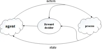
Reinforcement learning is based on the idea that the system learns directly from the inter-action during the process of approaching the goals. The reinforcement learning framework has five fundamental elements: agent, environment, state, reward, and action, showed as Fig. 1. In the reinforcement learning, an agent, which is also known as a controller, keeps interaction with the environment, generates a statest∈S, and chooses an actionat∈Ain accordance with a predetermined policyπsuch that atat=π(st). Consequently, the agent receive an immediate rewardrt+1=ρ(st,at) and gets to a new statest+1. By continuous trails and optimizing, the agent gets the maximal sum of the rewards as well as an optimal action sequence.
Fig. 1.Framework of reinforcement learning. The agent selects an action; the environment responds to the action, generates new scenes to the agent, and then returns a reward.
The goal of reinforcement learning is to maximize a long-term rewardR which is calculated by:
R= Eπ
r1+γr2+· · ·+γT−1rT +· · ·
= Eπ
(∞
X
t=1
γt−1rt
)
(1)
whereEπ is expectation of accumulation of the long term reward, and γ ∈(0,1] is a
discount factor increasing uncertainty on future rewards showing how far sighted the con-troller is in considering the rewards.
V (s) = Eπ
(∞ X
i=1
γi−1rt+i|st=s
)
= Eπ
(
rt+1+γ
∞
X
i=1
γi−1rt+i+1|st=s
)
=
∞
X
t=1
γtr(st) (2)
Reinforcement learning algorithms also use state state-action functionQ(s,a) which represents the accumulated long-term reward from a starting state. State-action function
Q(s,a) is defined as[15]:
Q(s, a) = Eπ
(∞
X
i=1
γi−1rt+i|st=s, at=a
)
= Eπ
(
rt+1+γ
∞
X
i=1
γi−1rt+i+1|st=s, at=a
)
=
∞
X
t=1
γtr(st, at) (3)
Despite that the state value functionV(s) and the state action value functionQ(s,a) represent long-term returns, they still can be expressed in a form that is relevant to the MDP model and the successive state or state action pair, called one step dynamic. In this way, it is not necessary to wait for the end of the episode to calculate the value of the corresponding value function, but to update the new value function in each step, so that the algorithm has the ability real-time online learning. In addition, the state value function and the state action value function also can be expressed as:
V(s) =
Z
a∈A
π(a|s)Q(s, a)da (4)
Q(s, a) =
Z
s0∈S
f(s0|s, a) [R(s, a, s0) +γV (s0)]ds (5)
As we can see that in the case where the environment model is completely known, the state value function and the state action value function can be transferred to each other seamlessly.
2.3. Policy Gradient
the policy iteration, the Qlearning [10], Sarsa algorithm [11] and LSPI algorithm [7]. The policy iteration algorithm computes the optimal policy by repeating policy evaluat-ing and policy improvevaluat-ing. The value function method is a generalized iterative algorithm, focusing on the solution of the state action of the value function, and then the strategy is calculated by the value function, commonly by greedy strategy. Unlike the value func-tion method, the policy gradient method represents the strategy directly through a set of policy parameters, rather than indirectly through the value function. The policy gradient method maximizes the cumulative reward function or the average reward by the gradient method to find out the optimal policy parameters, and each update is along the fastest rising direction of the reward function. The updates of policy parameters can be denoted as:
ψ=ψ+α∂Q(s, aψ) ∂uψ
∂uψ
∂ψ (6)
ψ=ψ+α∂R
∂ψ (7)
The gradient becomes zero when the reward function reaches the local optimal point. The core of the policy gradient method update is the solution of the gradient.
The updates of policy parameters in the policy gradient method can be categorized as deterministic policy and non-deterministic policy. A deterministic policy is a greedy strat-egy that can deal with continuous action space problems. Because reinforcement learning requires action exploration, deterministic policy cannot be applied individually to rein-forcement learning, often with some other method such asε-greedy method. The non-deterministic policy gradient can solve both discrete and continuous space problems, just being provided with strategy distribution in advance. The Gibbs distribution is often used for discrete space problems as:
π(a|s) = e
κ(s,a)Tψ
P
a0∈A
eκ(u,a0)Tψ (8)
While continuous space problem often takes advantage of Gaussian distribution, as:
π(a|s) =p 1
2πσ2(s)exp −
(a−µ(s))2 2σ2(s)
!
(9)
µ(s) =κ>µ(s)ψµ (10)
σ(s) =κ>σ(s)κσ (11)
whereκ(s,a) is the kernel of the state action pair (s,a),µ(s) is the mean value of the Gaussian distribution,σ(s)is the standard deviation of the Gaussian distribution,ψ =
performance. Therefore, in practice, the natural gradient method is used to replace the gradient method, so as to reduce the variance of the gradient, speed up the convergence rate of the algorithm and improve the convergence performance of the algorithm.
3.
Forward View and Backward View
As the most important part of the reinforcement learning method, the time difference (TD) method is an effective method to solve the long-term forecasting problem. However, the traditional TD methods have problems in matching forward view and backward view. In this section, we will state how to make the forward view equivalent to backward view, which is a very important foundation of the proposed algorithms.
3.1. Time Difference (TD)
TD method is one of the core algorithms of reinforcement learning. TD method, which is able to learn directly from the raw experience from an unknown environment and up-date the value function at any time without determining dynamic model of environment in advance. Temporal difference combines the advantages of Monte Carlo method and dy-namic programming. It updates the model by estimation based on part of learning rather than final results of the learning. Temporal difference works very well in dealing with real time prediction problems and control problems. Temporal difference learning updates by [15]:
V (st+1)←V(st) +α[Rt−V(st)] (12)
Q(st+1, a)←Q(st, a) +α[Rt−Q(st, a)] (13)
where Rt is return of step t, α is a step size parameter. Temporal difference learning updates V or Q in step t+ 1 using the observed reward rt+1 and estimated V(st+1)
Q(st+1,at+1)or .
One simple form of time difference algorithm, TD(0), updates the value function us-ing the estimated deviation of a statesat the two time points, before and after. As TD (0) algorithm updates the value function every step, rather than after all steps, the entire up-date process does not require environment information as many other algorithms do. This advantage of TD(0) algorithm makes it suitable for the online learning task under the un-known environment. In addition, as the value function updating of TD(0) doesn’t need to wait until the end of the episode, TD(0) can actually be used for non-episodic tasks, which sharply widens its application range compared to the Monte Carlo algorithm. The TD (0) algorithm is a method of evaluating the strategy. The Q learning algorithm and Sarsa algorithm are the two forms of TD(0).
3.2. TD(λ)
on the next state value function and the immediate reward is called a one-step update. Likewise, it is referred asn-step update if the update is based on the nextn steps. The
n-step update can be defined as:
R(t,ωn)=rt+1+γrt+2+· · ·+γn−1rt+n+γnω>κ(st+n) (14)
As theVfunction value of the current stateshas a variety of estimates, in the process of algorithm implementation, we often uses weighted average of the different n steps, which is calledλ-return:
Rλt = (1−λ) T−t−1
X
n=1
λn−1R(t,ωn)+λ T−t−1
Rt,ω(T−t) (15)
whereλis regarded as recession factor, andTis the maximum number of steps. It is called
λ-return algorithm when usingλ-return to update the current state value function:
ωt+1=ωt+α
Rλt −ω>κ(st)
κ(st) (16)
In the reinforcement learning, the above stated view is called forward view. Theλ -return algorithm cannot update value function until the end of the episode. Therefore,
λ-return algorithm uses the backward view to update the value function, which employs current TD error to update the value function of all states.
TD(λ) introduced the concept of the eligibility trace in backward view. The eligibility trace is essentially a record of the state or state of action recently visited. The cumulative eligibility trace can be defined as:
et=λγet−1+κ(st) (17)
In the backward view, the TD errorδtis updated according to the eligibility trace for
all state values, as:
ωt+1=ωt+αδtet (18)
The conventional forward calculatesλreturnRλ
t until the end of episode, while the
online forward view method is able to calculateλreturn at timet. This is called a truncated return, as:
Rλ|t 0
t = (1−λ) t0−t−1
X
n=1
λn−1Rt,ω(n)t+n−1+λ
t0−t−1R(t0−t)
4.
TOSarsa(
λ
) Algorithm
In the previous section, we have introduced how to achieve equivalence between for-ward view and backfor-ward view as well as its benefit of doing so. In this section, we will introduce a true online time difference algorithm which uses a clustering-based sample sparsification method [20] and selective kernel-based value function [4] as value function representation.
4.1. TOSarsa(λ) Algorithm Description
The true online time difference algorithm, named True Online State-action-reward-state-action(λ) (TOSarsa(λ)) is based on the effective Sarsa(λ) algorithm and uses Equation (17) as basic form of update equation to calculate eligibility trace, Equation (18) to cal-culate TD error and Equation (19) to calcal-culate return.
Algorithm 1True Online State-action-reward-state-action(λ) (TOSarsa(λ) )
Input: policy, threshold
Output: optimal policy
1: Initialize kernel functionκ(·,·) 2: Initialize sample setS 3: Set up data dictionaryD 4: repeat
5: Initialize starting states0
6: Initialize eligibility tracee←0 7: V(s)←ω>κ(s)
8: repeat
9: V(st+1)←ω>κ(st+1)
10: a←π(a|s) 11: Observer,s
12: δt←rt+1+γωt>κ(st+1)−ωt>−1κ(st)
13: et←γλet−1+αtκ(st)−αtγλ
e>t−1κ(st)
κ(st)
14: ωt+1←ωt+δtet+αt
ω>t−1κ(st)−ω>tκ(st)
κ(st)
15: ξ←minsi∈D(κ(s, s) +κ(si, si)−2κ(s, si))
16: UpdateD
17: ifξis greater than a predefined thresholdthen
18: V(st)←ω>κ(st+1)
19: Getωande
20: else
21: V(st)←V(st+1)
22: end if
23: st←st+1
24: untilall step of the current episode end 25: untilall episodes end
4.2. Mountain Car Problem
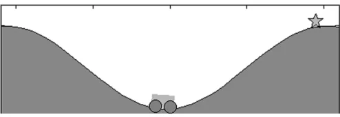
Mountain car problem [18] is a classic problem in strengthening learning, as shown in Fig. 2. The task of the car is to get to the top of the mountain, the right side of the ”star” mark position, as soon as possible. However, as the car is short of power, it is unable to drive to the top of the mountain directly. It has to accelerate back and forth many times to reach a higher position, and then accelerated to reach the end.
Fig. 2.Diagram of mountain car problem. The task of the car is to get to the top of the mountain, the right side of the ”star” mark position, as soon as possible.
We use MDP to model mountain car problem. In the mountain car problem, the state contains two dimensions, the position denoted by p and the speed denoted byv. Then
state of the car can be represented by a vectorx =
p v
. The acceleration of the car is
in the range of -1 to 1, that is, the actiona∈[-1,1]. The curve of the road surface can be expressed by the function
h=sin(3p) (20)
The state transition function can be expressed as
vt+1=bound[vt+ 0.001ut−0.0025 cos(3pt)] (21)
pt+1=bound[pt+ 1] (22)
whereboundis a function used to limited the value,bound(vt)∈[-0.07,0.07],bound(pt) ∈[-1.5, 1.5]. The coefficient of gravity acceleration direction is -0.0025.
Sarsa is an effective TD algorithm for control problems. We implemented the Sarsa version of the TOSarsa(λ) algorithm and compared with Sarsa and Sarsa(λ). Fig. 3 shows the control effect of the three algorithms on the initial state’s value function.
Fig. 3.The approximation effects of the algorithms on the initial state’s value function on the initial state’s value function.
which had a better strategy to evaluate performance was the best of three. However, all of the three algorithms had fluctuations at the beginning stage because at the initial stage, the data dictionary for the algorithms has not yet been completely established, and the algorithm kept exploration. We used TOSarsa(λ), Sarsa and Sarsa(λ) to solve the moun-tain car problem for 50 times. The results are shown in Fig. 4, where we can see that TOSarsa(λ) is the fastest in the three algorithms in the process of approximation. Fig. 4 shows the number of episodes required by the three algorithms, TOSarsa(λ), Sarsa and Sarsa(λ), to reach the target in different scenarios. TOSarsa(λ) was superior to the other two in the convergence rate and the convergence result. Moreover, the convergence result of TOSarsa(λ) was more stable.
5.
TOSarsa(
λ
) With Heuristic Dynamic Programming
The dual heuristic dynamic programming (DHDP) algorithm is a method of dealing with continuous action space by neural network. It applies the actor-critics framework, evalu-ates the strategy in the critics section, and calculevalu-ates deterministic strategies in the actors section. In this section, we will try to combine TOSarsa(λ) with heuristic dynamic pro-gramming.
5.1. TOSHDP Algorithm Description
The TOSarsa(λ) is used to evaluate the derivative of the value function to the state; update policy is updated by using the gradient descent method. The value of the function is:
λ(st) = ∂V(st)
∂st
=ω>κ(st) (23)
It satisfies the Bellman equation. We take TOSarsa (λ) method to get value ofλ(st) , TD error, as:
δt= ∂rt+1
∂st +γ
∂st+1
∂st + ∂st+1
∂at ∂at ∂st
ωtκ(st+1)−ωt−1κ(st) (24)
As it can be seen from the above equation, the Equation(24) needs to solve ∂st+1
∂st
and ∂st+1
∂at , which requires a complete information of environment or model. The dual
heuristic dynamic programming algorithm uses more environment knowledge and has a pretty good performance. In addition, the dual heuristic dynamic programming algorithm algorithm calculates the value of∂at
∂st, which is the actor part of the policy function of the
derivative. The policy parameters updating as follows:
ωt+1=ωt−β∆ωt
=ωt−β
∂V(st+1)
∂at ∂at ∂ωt
=ωt−βλ(st+1)
∂st+1
∂ut ∂at ∂ωt
=ωt−βλ(st+1)
∂st+1
∂at κ(st) (25)
whereβis learning step for policy parameters. The following is the algorithm of TOSarsa(λ) with heuristic dynamic programming, where the8thstep of the algorithm is the
combina-tion of optimal policy funccombina-tion andε-greedy.
5.2. Cart Pole Balancing Problem
Algorithm 2TOSarsa(λ) with heuristic dynamic programming (TOSHDP)) )
Input: policy, threshold
Output: optimal policy 1: Initialize sample setS 2: Set up data dictionaryD 3: repeat
4: Initialize starting states0
5: Initialize eligibility tracee←0 6: λ(st)←ω>κ(st)
7: repeat
8: a←π(a|s) 9: Observer,s
10: λ(st+1)←ω>κ(st+1)
11: δt←rt+1+γ
∂s
t+1
∂st +
∂st+1
∂at
∂at
∂st
λ(st+1)−λ(st)
12: et←γλet−1+αtκ(st)−αtγλe>t−1κ(st)κ(st)
13: ωt+1←ωt−βλ(st+1) ∂st+1
∂at κ(st)
14: ξ←minsi∈D(κ(s, s) +κ(si, si)−2κ(s, si))
15: UpdateD
16: ifξis greater than a predefined thresholdthen
17: V(st)←ω>κ(st+1)
18: Getωande
19: else
20: V(st)←V(st+1)
21: end if
22: st←st+1
23: untilall steps of the current episode end 24: untilall episode end
25: return optimal policy
m=1kg, the lengthl = 1m. The pole and the car are hinged together. The pole and the vertical direction are at an angle. In order to make the angle of the pole and the vertical direction in[−36◦,36◦], where the angle is negative if the pole is on the left side of the vertical line, and the angle is positive if the pole is on the right side of the vertical line. After each time interval∆t= 0.1s, a horizontal forceFis applied to the cart, whereFis within [-50N, 50N] (negative means the force is to the left, and positive is to the right), and there is a random noise disturbance between [-10N, 10N] whenFis applied. All frictional forces were not considered. The task of the agent is to learn a policy so that the angle between the pole and the vertical direction is kept as much as possible in the specified range.
We use MDP to model the cart pole balancing problem. The state of the environment is represented by two variablesαandβ, whereαis the angle formed by the pole and the vertical line, andβis the angular acceleration of the rod. The state space is:
S ={(α, β)|α∈[−36◦,36◦], β∈[−36◦,36◦]} (26)
Fig. 5.Cart pole balancing problem diagram.
A={a|a∈[−50N,50N]} (27)
Agent exerts forceFon the cart, and the angular acceleration of the pole is:
ξ=
gsinα+ cosα−f−mmlβ+M2sinθ
l4 3−
mcos2α
m+M
(28)
wheregis the constant of gravitational acceleration, with value 9.81m/s2; andf is the value of forceF. After∆t, the states areα=β+ξ∆t,β =α+β∆t, and the reward function is
ρ(x, u) =
1,|f(x, u)|<36◦
−1,|f(x, u)| ≥36◦. (29)
The episode ends when the angle between the pole and the vertical line exceeds the given range. If the pole has not fallen and kept standing after 3000 time steps, it is regarded as a successful trial.
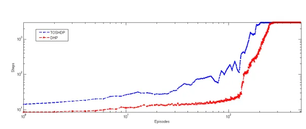
We compare TOSHDP with conventional DHP algorithm, where DHP uses two three-layer neural networks for value functions and policy approximation, all of their learning steps are 0.1. The results are shown in Fig. 6.
Fig. 6.Results of TOSHDP vs. conventional DHP algorithm where the value of the learn-ing steps were set as 0.1.
6.
Conclusion
We propose a true online kernel time difference algorithm, TOSarsa(λ), which employs a clustering-based sample sparsification method and selective kernel-based value function as value function representation. The experiment on mountain car problem showed our algorithm was effective in deal with the typical continuous problems and could speed up strategy search as well.
We combined the proposed TOSarsa(λ) algorithm with the dual heuristic dynamic programming algorithm to improve policy learning speed of policy search algorithms by replacing approximating using neural network method with approximating using kernel method. The experiment on cart pole balancing problem verified that our proposed algo-rithm really worked. It is a good alternative to deal with continuous action space problems. However, there is still some work to study further, such as how to extend the model to deal with the continuous space problems of unknown environment.
Acknowledgments.This paper is supported by National Natural Science Foundation of China (61303108, 61373094,61772355, 61702055,61602332), Jiangsu Province Natural Science Research University major projects (17KJA520004), Suzhou Industrial application of basic research program part (SYG201422), Provincial Key Laboratory for Computer Information Processing Technology of Soochow University (KJS1524), China Scholarship Council project (201606920013).
References
1. Al-Rawi A, Ng A, Y.A.: Application of reinforcement learning to routing in distributed wireless networks: a review. Artificial Intelligence Review 43(3), 381–416 (2015)
2. Bagnell A, Ng Y, S.J.: Policy search by dynamic programming. In: Advances in Neural Infor-mation Processing Systems. pp. 831–838 (2004)
3. Busoniu L, Babuska R, e.a.: Reinforcement learning and dynamic programming using function approximators. CRC Press (2010)
5. E., B.: A markov decision process. Journal of Mathematical Fluid Mechanics 6(1), 65–73 (1957)
6. El I, Feng M, e.a.: Reinforcement learning strategies for decision making in knowledge-based adaptive radiation therapy: application in liver cancer. International Journal of Radiation On-cology Biology Physics 96(2), 38–45 (2016)
7. Ghorbani F, Derhami V, A.M.: Fuzzy least square policy iteration and its mathematical analysis. International Journal of Fuzzy Systems 19(13), 1–14 (2016)
8. H., V.H.: Reinforcement learning, chap. Reinforcement learning in continuous state and action spaces, pp. 207–251. Springer Berlin Heidelberg (2012)
9. K., D.: Reinforcement learning in continuous time and space. Neural Computation 12(1), 210– 219 (2000)
10. Kiumarsi B, Lewis L, e.a.: Reinforcement q-learning for optimal tracking control of linear discrete-time systems with unknown dynamics. Automatica 50(4), 1167–1175 (2014) 11. Kober J, Bagnell A, P.J.: Reinforcement learning in robotics: a survey. The International Journal
of Robotics Research 32(11), 1238–1274 (2013)
12. L, P.: Markov decision processes: discrete stochastic dynamic programming. John Wiley and Sons (2014)
13. M., H.: Value-function approximations for partially observable markov decision processes. Journal of Artificial Intelligence Research 13(1), 33–94 (2011)
14. Scholkopf B, Platt J, H.T.: An application of reinforcement learning to aerobatic helicopter flight. In: Advances in Neural Information Processing Systems. vol. 19, pp. 1–8. Proceedings of the Twentieth Conference on Neural Information Processing Systems, Vancouver, British Columbia, Canada (2007)
15. Sutton R, B.G.: Reinforcement learning : an introduction. IEEE Transactions on Neural Net-works 16(1), 285–286 (2005)
16. Sutton R, Mcallester D, e.a.: Policy gradient methods for reinforcement learning with function approximation. In: Advances in Neural Information Processing Systems. vol. 12, pp. 1057– 1063 (2000)
17. T., P.: Solving the pole balancing problem by means of assembler encoding. Journal of Intelli-gent and Fuzzy Systems 26(2), 857–868 (2014)
18. Whiteson S, Tanner B, W.A.: The reinforcement learning competitions. AI Magazine 31(2), 81–94 (2010)
19. Yau A, Goh G, e.a.: Application of reinforcement learning to wireless sensor networks: models and algorithms. Computing 97(11), 1045–1075 (2015)
20. Zhu H, Zhu F, e.a.: A kernel-based sarsa(λ) algorithm with clustering-based sample sparsifi-cation. In: International Conference on Neural Information Processing. pp. 211–220. Springer International Publishing (2016)
Fei Zhuis a member of China Computer Federation. He is a PhD and an associate pro-fessor. His main research interests include machine learning, reinforcement learning, and bioinformatics.
Haijun Zhuis a postgraduate student in the Soochow University. His main research in-terest is reinforcement learning. He programmed the algorithms and implemented the experiments.
Donghuo Chenis a member of China Computer Federation. He is a PhD. His research interest includes reinforcement learning, model checking.
Xiaoke Zhouis now an assistant professor of University of Basque Country UPV/EHU, Faculty of Science and Technology, Campus Bizkaia, Spain. He majors in computer sci-ence and technology. His main interests include machine learning, artificial intelligsci-ence and bioinformatics.