Estimation of Input Function from Dynamic PET Brain
Data Using Bayesian Blind Source Separation
Ondˇrej Tich´y and V´aclav ˇSm´ıdl
Institute of Information Theory and Automation, Pod Vod´arenskou Vˇeˇz´ı 4, Prague, Czech republic
{otichy,smidl}@utia.cas.cz
Abstract. Selection of regions of interest in an image sequence is a typical pre-requisite step for estimation of time-activity curves in dynamic positron emission tomography (PET). This procedure is done manually by a human operator and there-fore suffers from subjective errors. Another such problem is to estimate the input function. It can be measured from arterial blood or it can be searched for a vascular structure on the images which is hard to be done, unreliable, and often impossible. In this study, we focus on blind source separation methods with no needs of manual in-teraction. Recently, we developed sparse blind source separation and deconvolution (S-BSS-vecDC) method for separation of original sources from dynamic medical data based on probability modeling and Variational Bayes approximation method-ology. In this paper, we extend this method and we apply the methods on dynamic brain PET data and application and comparison of derived algorithms with those of similar assumptions are given. The S-BSS-vecDC algorithm is publicly available for download.
Keywords:blind source separation, variational Bayes method, dynamic PET, input function, deconvolution
1.
Introduction
Physical examination using scintigraphy [6] or positron emission tomography (PET) [11] allows us to see processes inside the living body without surgery. Contrast medium can be applied into the body and its spatial distribution can be measured for the selected part of body. In PET, the measured activity in each voxel is a superposition of the signal tissues. Since the measurement is done repetitively, a time distribution of the scanned region of body can be obtained. The task of medical analysis is to obtain the clear activity of each tissue separately.
However, more important problem is that the selected blood structure typically accu-mulate activity not only from the blood but also from other tissues; hence, a mixture of TACs is obtained instead of the pure IF. Moreover, such a structure is often not present on scanned images and no such ROI with pure IF can be placed. Separation of mixed signals in general is the task for blind source separation (BSS) methods. They offer an automatic way for separation of tissues from the measured sequence. Some methods are general with no extra medical assumptions [21,3] and provide non-negative matrix factorization essentially [17,7]. Medically motivated extensions have been proposed based on compart-mental modeling [23,31] where detailed model of the tracer behavior is incorporated into the separation procedure.
Recently, we have studied the influence of the sparsity assumption on BSS problems, which means to reflect that the activity of each source is present only on limited region of recorded images [14]. We developed sparsity in blind source separation and detion (S-BSS-vecDC) method [29] which assumes each TAC to be the results of a convolu-tion between common input funcconvolu-tion and specific convoluconvolu-tion kernel and source-images to be sparse. The sparsity is not strict but favored by proposed probabilistic model using automatic relevance determination principle [2]. Suitability of the S-BSS-vecDC algorithm was studied on dynamic PET in [28]. In this paper, we extend the comparison by adding a method that estimates the full covariance matrix of the convolution kernels using Wishart prior model [30].
We compare the proposed and existing methodology on the task of tissue separation of the TAC of the blood. Specifically, we analyze data from dynamic PET of a brain where structures with arterial blood are obvious and thus this data can be used as the simplest possible benchmark of separation methods. The comparison is performed for two cases: slice by slice processing and the whole volume processing. It allows us to study the separation performance as well as stability of the algorithms.
The structure of the paper follows. In Section 2, related work on blind source separa-tion in context of dynamic PET data analysis is discussed. In Secsepara-tion 3, models for blind source separation are introduced, three classical models without any specific domain as-sumptions and three models with convolution assumption. Variational Bayes method for estimation of models parameters is described in the end of the Section. In Section 4, an experiment with dynamic PET brain data is conducted slice by slice and for the whole volume while the estimated blood sources are compared with the manually obtained esti-mate. In Section 5, discussion and conclusion are given.
2.
Related Work
and some of them are used by their authors but, again, none has been generally accepted in general clinical practice.
Promising model of dynamic PET images is the one where it is assumed that data are superposition of signals from several sources while each source image is weighted by its related time-activity curve. This model is the base for non-negative matrix factorization [17] which was already applied to PET data [3]. This model was improved using addi-tional assumptions such as sparsity [13] or convolution assumption [24]; however, noise properties and unknown number of source remain issues. Similar model was proposed in [9] to solve near-separable non-negative matrix factorization where it is assumed that each source has at least one clear image in the data. This assumption is suitable for wide class of problems but limits this algorithm in medical data analysis. We tried to overcome these issues using Bayesian approach in [26] where sparsity of source images was modeled and in [31] where convolution assumption was incorporated and piece-wise linear convolution kernels was modeled. These algorithms provide good results in domain-specific tasks. To overcome dependency on domain, free-form approach was pioneered in [27] using auto-matic relevance determination principle [2] and S-BSS-vecDC algorithm was proposed in [29] where noise level as well as number of sources are estimated within Bayesian model and sparsity of source images and convolution model was incorporated using general, i.e. no domain-specific, assumptions. This algorithm will be tested and compare with other algorithms in this paper.
3.
Blind Source Separation Methods
The general assumptions of the blind source separation methods, which is common for all methods to be compared, will be summarized. Then, we will make detailed views on the selected methods.
The observed data are assumed to arise as a superposition of signals from underlying tissues and the signal is assumed to be degraded by a noise. The data at each time t
is stored columnwise in vectordt. Since the number of voxels is p,dt ∈ Rp×1. The
vectordtis assumed to be an observation of a superposition ofrtissue images stored in vectorsak ∈Rp×1, k= 1, . . . , r. Each tissue image is weighted by its related TACxk ∈
Rn×1, k = 1. . . , r, wherenis the number of measurements,t= 1, . . . , n. Summarizing
the vectors into matricesD = [d1, . . . ,dn] ∈ Rp×n,A = [a1, . . . ,ar] ∈ Rp×r, and
X = [x1, . . . ,xr]∈Rn×r, the matrix formulation of the superposition problem can be
written as
D=AXT +E. (1)
Here()T denotes transpose of a matrix or vector andE is the noise matrix of the same size as the data matrixD.
3.1. Non-negative Matrix Factorization
Non-negative matrix factorization (NMF) assumes that the data matrixD ∈ Rp×n can
be approximated by linear combinationD ≈AXT, whereA ∈R+p×r, andX ∈Rn+×r
is TACs recovering the columns ofD using the columns ofA. The number of sources,
distance measuring the quality of the approximation of the matrices D by the product
AXT defined as
||D−AXT||2=
∑
i,j (
Dij−(AXT)ij
)2
, (2)
where the convergence to a local optimum is guaranteed [18].
3.2. Blind Source Separation with Positivity
Additional biologically-motivated assumptions are imposed on the elements of (1) in the probabilistic model of Blind Source Separation with Positivity (BSS+): (i) all elements of the observed vectorsdtare positive, (ii) all elements of the tissue imagesak and the
TACsxkare also positive, and (iii) the number of relevant sources,r, is unknown. These
assumptions are translated into probabilistic model as described in [21]. Moreover, the variance of noise is estimated as well as the relevant number of vectors,r, using automatic relevance determination (ARD) mechanism [2].
3.3. Factor Analysis with Integrated Regions of Interests
The Factor Analysis with Integrated Regions of Interests (FAROI) method [26] has the same advantage as BSS+ method; however, tissue images are modeled in more detail. Each element of matrixA,ai,k, has indicatorii,ksuch as
ii,k=
{
1 i-th pixel belongs to the k-th tissue
0 i-th pixel not belongs to the k-th tissue (3)
and then, the model for each pixel depends on the indicator as
f(ai,j) =
{
U(0,1) ii,j= 1,
tN(0, ξ−j1,⟨0,1⟩) ii,j= 0.
(4)
Here, uniform distributionU(0,1)is a model of the tissue and the truncated normal dis-tributiontN(0, ξj−1), defined in Appendix A.1, models the noise around zero.
As a result, the FAROI model is capable to separate tissue images with small number of pixels which could be rejected as insignificant by the BSS+ model.
3.4. Blind Compartment Model Separation
The Blind Compartment Model Separation (BCMS) model [31] reflects that the TACs can be described by compartment model, where each TAC arise as a convolution between a common input function and a tissue-specific kernel [23,15]. Hence, each element of the matrixX,xj,k, is modeled as a convolution between the input function, vectorb, and the
convolution kerneluksuch as
xj,k=
j ∑
t=1
Since we define the matrixU = [u1, . . . ,ur]∈Rn×rand the matrixBas B=
b1 0 0 0
b2 b1 0 0
. . . b2 b1 0
bn . . . b2b1
, (6)
the matrixXof all TACs can be rewritten as
X =BU, (7)
and matricesUandBare now unknown parameters instead of the matrixX.
In the BCMS model, the input functionbis assured to be decreasing and kernelsuk
are assured to be decreasing and piece-wise linear with constant plateau in the beginning and the decreasing to zero [15]. All these assumption are formulated as prior distribution on model parameters and the model is solved using Variational Bayes method [25].
The limitation of BCMS method is its restrictive shape which is suitable only in lim-ited number of situation such as in specific tasks in renal scintigraphy [31].
0510152025303540 0 0.01 0.02 0.03 0.04 0.05 0.06 0.07 0.08
0510152025303540 0 0.2 0.4 0.6 0.8 1 1.2 1.4 0510152025303540 0 2 4 6 8 10 12 14 16 18
0510152025303540 0 500 1000 1500 2000 2500 3000 3500 4000 4500
Input function and convolution kernels estimation
Time
Initialization
Source images estimation
Iterative Algorithm Source Time−Serie
− Probabilistic model formulation − Sparsity using hierarchical priors
− Number of sources estimation − Check the stopping rule − Noise level estimation − Estimation of variance of noise
− Number of sources estimation
PET
example res.
Results
source image convolution kernel time−activity curve
= * example res. scintigraphy Subsequent Analysis PET MRI scintigraphy
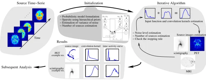
Fig. 1.The flowchart of the methods with incorporated convolution model.
3.5. Sparsity in Blind Source Separation and Deconvolution
Sparse Blind Source Separation and Deconvolution (S-BSS-vecDC) method [29] applies the automatic relevance determination (ARD) mechanism [2] to more variables of the model. The convolution model of TACs (7) is also adopted; however, in a more relaxed form than in the BCMS method. The convolutions kernels are not restricted to be in piece-wise linear form, the only imposed assumption is their sparsity via the ARD methodology:
f(uj,k|υj,k) =tN(0, υj,k−1,[0;∞]), ∀j= 1, . . . , n, (8)
Hence, each element of the convolution kernel is truncated to positive value, see Appendix A.1, and its varianceυj,k is modeled as a Gamma prior and estimated jointly with the convolution kernel.
The sparsity prior is also used for each elementai,kof tissue images, matrixA, as
f(ai,k|ξi,k) =tN(0, ξi,k−1,[0; 1]), ∀i= 1, . . . , p, (10)
f(ξi,k) =G(ϕ0, ψ0). (11)
Note that in this case, the normal distribution (10) is truncated to real numbers from the interval[0; 1]which results in better stability of its solution.
The input function model is modeled as
f(b|ς) =tN(0n,1, ς−1In), f(ς) =G(ζ0, η0), (12)
whereς is scaling parameter andζ0, η0are scalar chosen constants.
The probabilistic model is solved using Variational Bayes method [25]. The algorithm implemented in MATLAB can be downloaded from
http://www.utia.cas.cz/AS/softwaretools/image_sequences.
3.6. Blind Source Separation with Wishart Convolution Prior
Fig. 2.The used localization matrixLin S-BSS-DW model. The black pixels denote ones
and the white pixels denote zeros;n= 10andr= 4.
Fixed-form convolution kernels has been studied in Section 3.4 in BCMS method, and free-form sparse convolution kernels has been studied in Section 3.5 in S-BSS-vecDC method. In S-BSS-vecDC method, covariance matrix of convolution kernels is assumed to be diagonal in prior model (8). As an extension, we have studied a full prior covariance matrix of convolution kernels using Wishart distribution.
In vector notation, the convolution kernels are stored in one vector asu= vec(U) =
u1
.. .
ur
tN(0nr,1,diag(υ1, . . . ,υr)−1 )
. The restriction of diagonal shape of the covariance ma-trix is here omitted using model
f(u|Υ) =tN(0nr,1, Υ−1
)
, (13)
where matrixΥ ∈Rnr×nris a full covariance matrix of vectoru[30]. The matrixΥ is
modeled as the Wishart distribution, see Appendix A.2,
f(Υ) =Wnr(α0Inr, β0), (14)
with scalar prior parametersα0, β0. The models of source images and the input function
remain the same as given in equations (10)–(12).
Using this model, the full covariance matrix of the convolution kernels could be es-timated; however, the model is then overparametrized since additionaln2r2parameters need to be estimated. To overcome this problem, we use an empirical observation that the most information is located in a few main diagonals of the covariance matrix. This approach is known as the localization and originates in data assimilation of atmospheric models [12]. Here, the estimate of the covariance matrix of theu,Υb, is localized using the matrixLof the same size as
b
Υloc=Υb◦L, (15)
where symbol◦denotes the Hadamard product, also known as the element-wise product, and the matrixLis defined in Figure 2. Theoretically, we can construct any conceivable matrixL; however, the matrix for preservation of the three main diagonals is used in this study.
Once again, the probabilistic model is solved using Variational Bayes method [25]. The method is called Sparse Blind Source Separation and Deconvolution with Wishart Prior (BSDW). The flowchart of the methods with convolution model (BCMS, S-BSS-vecDC, and S-BSS-DW) is illustrated in Figure 1.
3.7. Approximate Variational Bayes Solutions
Estimation procedure for each prior model is derived using the Variational Bayes method [25]. The key step of the method is a replacement of intractable evaluation of joint poste-rior distribution by an approximate conditional independent distributions such as
f(A,b,u, ω|D)≈f(A|D)f(b|D)f(u|D)f(ω|D), (16)
where this example is for a model with convolution model of TACs. Following this methodology, shaping parameters of posterior distributions of model parameters are found using iterative procedure solving a set of derived implicit equations. The scheme of the methods with convolution model (BCMS, S-BSS-vecDC, S-BSS-DW) is shown in Figure 1.
4.
Experiments
Tissue Image
0 10 20 30 40 0 0.1 0.2 0.3 Image no. Activity TAC
0 10 20 30 40 0
0.1 0.2
Image no.
Activity
0 10 20 30 40 0
0.1 0.2
Image no.
Activity
0 10 20 30 40 0 0.1 0.2 0.3 Image no. Activity Tissue Image
0 10 20 30 40 0 0.1 0.2 0.3 Image no. Activity TAC
0 10 20 30 40 0
0.1 0.2
Image no.
Activity
0 10 20 30 40 0
0.1 0.2
Image no.
Activity
0 10 20 30 40 0 0.1 0.2 0.3 Image no. Activity Tissue Image
0 10 20 30 40 0 0.1 0.2 0.3 Image no. Activity TAC
0 10 20 30 40 0
0.1 0.2
Image no.
Activity
0 10 20 30 40 0
0.1 0.2
Image no.
Activity
0 10 20 30 40 0 0.1 0.2 0.3 Image no. Activity
BSS+ FAROI NMF
Tissue Image
0 10 20 30 40
0 0.1 0.2 0.3 Image no. Activity TAC
0 10 20 30 40
0 0.1 0.2
Image no.
Activity
0 10 20 30 40
0 0.1 0.2
Image no.
Activity
0 10 20 30 40
0 0.1 0.2 0.3 Image no. Activity Tissue Image
0 10 20 30 40
0 0.1 0.2 0.3 Image no. Activity TAC
0 10 20 30 40
0 0.1 0.2
Image no.
Activity
0 10 20 30 40
0 0.1 0.2
Image no.
Activity
0 10 20 30 40
0 0.1 0.2 0.3 Image no. Activity Tissue Image
0 10 20 30 40
0 0.1 0.2 0.3 Image no. Activity TAC
0 10 20 30 40
0 0.1 0.2
Image no.
Activity
0 10 20 30 40
0 0.1 0.2
Image no.
Activity
0 10 20 30 40
0 0.1 0.2 0.3 Image no. Activity
BCMS S−BSS−vecDC S−BSS−DW
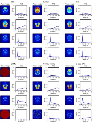
Fig. 3.The example results from the BSS+, FAROI, BCMS, NMF, BSvecDC, and
In this study,18F-altanserin was applied to a patient and scanned with an 18-ring
GE-Advance scanner (General Electric Medical System, Milwaukee, WI, USA) which is able to record 3D scans. Each scan consists of 35 image slices with an interslice distance 4.25 mm. The data were reconstructed into a sequence of128×128×35voxel matrices,
2×2×4.25mm each voxel, using software provided by the manufacturer. The sequence consists of40voxel matrices,n= 40. For illustration of the method, we selected the 10th slice; however all algorithms can proceed the full volume.
Separation of the tissue images on the 10th slice using BSS+, FAROI, BCMS, NMF, S-BSS-vecDC, and S-BSS-DW algorithms are displayed in Figure 3 withr = 4. Note that the tissues separated by the S-BSS-vecDC algorithm have better anatomical meaning than those from the competing methods. The first tissue is clearly separated by the S-BSS-vecDC and S-BSS-DW algorithms while there is a residual activity from arterial veins by the BSS+ and the FAROI algorithms and from both, arterial veins and the second tissue, by the NMF algorithm. The BCMS algorithm was not able to separate the first tissue. The third tissue, arterial veins, is again clearly separated by the vecDC and S-BSS-DW algorithms while the BSS+, the FAROI, and the NMF algorithms split the arterial veins into two tissues mixed with the artifacts of the PET reconstruction. The BCMS algorithm combines the first tissue into the third tissue which can be recognized from its TAC. Moreover, the S-BSS-vecDC algorithm clearly separated the PET reconstruction artifacts as the forth estimate; hence, the previous three physiological tissues are cleared from these artifacts.
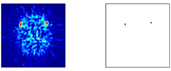
Fig. 4.The source image forn= 9is displayed on the left image. The manually selected
ROIs of arterial veins are displayed on the right image.
0 10 20 30 40 0
0.05 0.1 0.15 0.2 0.25
Image no.
Activity
BSS+ FAROI BCMS NMF S−BSS−vecDC S−BSS−DW Manual
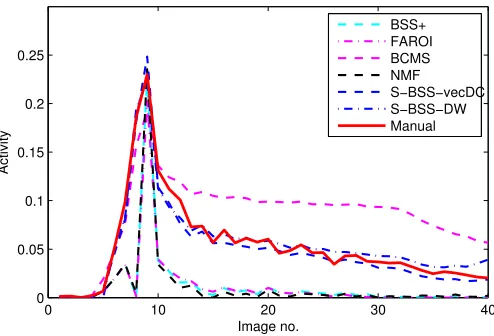
Fig. 5.Estimated TACs of blood tissue for the selected slice from all comparing methods
are shown.
4.1. Input Function Estimation from Slices
The goal of this experiment is to estimate input function from the whole measured volume. Firstly, we created a manual ROI in several slices in the same sense as in Figure 4. We obtained a manually derived TAC of blood using this approach. Note that the TAC of the blood that was obtained manually is supposed to be slightly overestimated over the true blood curve since it contains signal from other tissues. This TAC will be used for comparison with the blood estimates from the BSS+, FAROI, NMF, and S-BSS-vecDC algorithm. Secondly, we ran the studied automatic algorithms on the whole volume slice by slice and the blood curves were selected from the results for each slice and for each algorithm. The results are displayed in Figure 6 using mean value and standard deviation at each time point. The curves are compared with manually obtained blood TAC, the red line.
The results in Figure 6 show that estimates from the S-BSS-vecDC algorithm are sys-tematically closer to the manual method than estimates from any other algorithm. Note that the estimates from the DW algorithm are closer to those from the S-BSS-vecDC algorithm; however, there is deviation from the manual curve in the increasing part of the blood curve in the beginning of the activity. The small disproportion between man-ually obtained blood TAC and blood TAC from the S-BSS-vecDC algorithm is expected since manually selected ROI always contains other tissues and therefore accumulate ac-tivity from them.
4.2. Input Function Estimation from the Whole Volume
0 10 20 30 40 0
0.1 0.2 0.3 0.4
Image no.
Activity
BSS+
0 10 20 30 40
0 0.1 0.2 0.3 0.4
Image no.
Activity
FAROI
0 10 20 30 40
0 0.1 0.2 0.3 0.4
Image no.
Activity
NMF
0 10 20 30 40
0 0.1 0.2 0.3 0.4
Image no.
Activity
BCMS
0 10 20 30 40
0 0.1 0.2 0.3 0.4
Image no.
Activity
S−BSS−vecDC
0 10 20 30 40
0 0.1 0.2 0.3 0.4
Image no.
Activity
S−BSS−DW
Fig. 6.The calculated mean and standard deviation of blood TAC for the BSS+, FAROI,
NMF, BCMS, S-BSS-vecDC, and S-BSS-DW algorithms are displayed. The red curve is blood TAC obtained using manually placed ROI.
0 10 20 30 40
0 0.05 0.1 0.15 0.2 0.25 0.3 0.35
0 10 20 30 40
0 0.05 0.1 0.15 0.2 0.25 0.3 0.35
Fig. 7.Illustration of the boundary value problem observed for methods with convolution
model of the TACs.Left:estimate of the blood TAC without data preprocessing.Right:
20 40 60
0 10 20 30 40 0 0.1 0.2 0.3 0.4 Image no. Activity BSS+ 20 40 60
0 10 20 30 40 0 0.1 0.2 0.3 0.4 Image no. Activity FAROI 20 40 60
0 10 20 30 40 0 0.1 0.2 0.3 0.4 Image no. Activity NMF 20 40 60
0 10 20 30 40 0 0.1 0.2 0.3 0.4 Image no. Activity BCMS 20 40 60
0 10 20 30 40 0 0.1 0.2 0.3 0.4 Image no. Activity S−BSS−vecDC 20 40 60
0 10 20 30 40 0 0.1 0.2 0.3 0.4 Image no. Activity S−BSS−DW
Fig. 8.Estimates of the blood tissue in the PET sequence composed of pixels belonging
to the blood on the left and their time activity on the right. Results of the BSS+ (top left), FAROI (top middle), NMF (top right), BCMS (bottom left), S-BSS-vecDC (bottom middle), and S-BSS-DW (bottom right) algorithms from the full volume are shown. The red curve is the TAC of the blood obtained using manually placed ROI.
run the algorithms for the whole volume. We will study if the behavior of the TACs of the blood will vary from those obtained slice by slice.
Here, the boundary value problem known e.g. from deblurring in image processing [20] was observed by the models with incorporated convolution model of TACs, see ex-ample of this effect in Figure 7, left, where residual activity is observed at the end of the TAC. To overcome this problem, we use preprocessing of the data. Specifically, we enlarge the original sequence using the last image with activity decreased by a small co-efficient. This extension is processed and the results are truncated to the original domain, see Figure 7, right.
Comparison of estimates of the blood tissue is displayed in Figure 8 accompanied by following mean absolute error (MAE) between estimated blood curves and manually obtained blood curve. The BSS+ result (MAE 0.044) is on the top left, the FAROI result (MAE 0.044) is in the top middle, the NMF result (MAE 0.042) is on the top left, the BCMS result (MAE 0.031) is on the bottom left, the S-BSS-vecDC result (MAE 0.015) is on the bottom middle, and the S-BSS-DW result (MAE 0.021) is on the bottom right. All algorithms provide stable estimates of the blood TAC, however the result of the S-BSS-vecDC algorithm are closest to the expected value. All blind source separation algorithms provide slightly lower estimates of the blood TAC than the manual method which could be caused by additional background tissue activity in manually selected ROI of the blood.
5.
Discussion and Conclusion
of activity in the blood which could be reliably estimated manually for this data and thus it can be used as a good reference value.
From the results of separation provided by these six methods, we manually selected the sources corresponding to the blood stream and compare their time-activity curves with the manually obtained reference. Our S-BSS-vecDC method [29] outperforms other meth-ods in proximity of its estimates to the reference ones. Agreements of this method with manual selection is very encouraging and has the potential to replace invasive estimation of the blood curve used as the input function in various applications.
Acknowledgement. This work was supported by the Czech Science Foundation, grant No. 13-29225S.
A.
Required Probability Distributions
A.1. Truncated Normal Distribution
Truncated normal distribution, denoted astN, of a scalar variablexon interval[a;b]is defined as
x∼tN(µ, σ,[a, b]) =
√
2 exp((x−µ)2)
√
πσ(erf(β)−erf(α))χ[a,b](x), (17)
whereα = a√−µ
2σ, β = b−µ
√
2σ, function χ[a,b](x)is a characteristic function of interval
[a, b] defined asχ[a,b](x) = 1if x ∈ [a, b] andχ[a,b](x) = 0otherwise. erf()is the
error function defined as erf(t) = √2
π
∫t
0e−
u2du. The moments of truncated normal
distribution are
b
x=µ−√σ
√
2[exp(−β2)−exp(−α2)]
√
π(erf(β)−erf(α)) , (18)
c
x2=σ+µbx−√σ
√
2[bexp(−β2)−aexp(−α2)]
√
π(erf(β)−erf(α)) . (19)
See [27] for multivariate extention.
A.2. Wishart Distribution
Wishart distributionWof the positive-definite matrixX ∈Rp×pis defined as
Wp(Σ, ν) =|X|
ν−p−1
2 2−
νp
2 |Σ|−ν2Γ−1
p
(ν
2
)
×exp
(
−1
2tr
(
Σ−1X)), (20)
whereΓp
(ν
2
)
is the gamma function. The required moment is:
b
References
1. Alf, M., Wyss, M., Buck, A., Weber, B., Schibli, R., Kr¨amer, S.: Quantification of brain glucose metabolism by18F-FDG PET with real-time arterial and image-derived input function in mice. Journal of Nuclear Medicine 54(1), 132–138 (2013)
2. Bishop, C., Tipping, M.: Variational relevance vector machines. In: Proceedings of the 16th Conference on Uncertainty in Artificial Intelligence. pp. 46–53 (2000)
3. Bodvarsson, B., Hansen, L., Svarer, C., Knudsen, G.: Nmf on positron emission tomography. In: Acoustics, Speech and Signal Processing, 2007. ICASSP 2007. IEEE International Confer-ence on. vol. 1, pp. I–309. IEEE (2007)
4. Calamante, F., Mørup, M., Hansen, L.: Defining a local arterial input function for perfusion mri using independent component analysis. Magnetic resonance in Medicine 52(4), 789–797 (2004)
5. Croteau, E., Poulin, E., Tremblay, S., Dumulon-Perreault, V., Sarrhini, O., Lepage, M., Lecomte, R.: Arterial input function sampling without surgery in rats for positron emission tomography molecular imaging. Nuclear medicine communications 35(6), 666–676 (2014) 6. Di Paola, R., Bazin, J., Aubry, F., Aurengo, A., Cavailloles, F., Herry, J., Kahn, E.: Handling of
dynamic sequences in nuclear medicine. Nuclear Science, IEEE Transactions on 29(4), 1310– 1321 (1982)
7. Gaujoux, R., Seoighe, C.: Semi-supervised nonnegative matrix factorization for gene expres-sion deconvolution: a case study. Infection, Genetics and Evolution 12(5), 913–921 (2012) 8. Germano, G., Chen, B., et al.: Use of the abdominal aorta for arterial input function
determina-tion in hepatic and renal pet studies. Journal of nuclear medicine 33(4), 613 (1992)
9. Gillis, N.: Successive nonnegative projection algorithm for robust nonnegative blind source separation. SIAM Journal on Imaging Sciences 7(2), 1420–1450 (2014)
10. Greuter, H., Boellaard, R., et al.: Measurement of 18f-fdg concentrations in blood samples: comparison of direct calibration and standard solution methods. Journal of nuclear medicine technology 31(4), 206–209 (2003)
11. Gunn, R., Gunn, S., Cunningham, V.: Positron emission tomography compartmental models. Journal of Cerebral Blood Flow & Metabolism 21(6), 635–652 (2001)
12. Hamill, T., Whitaker, J., Snyder, C.: Distance-dependent filtering of background error covari-ance estimates in an ensemble kalman filter. Monthly Weather Review 129(11), 2776–2790 (2001)
13. Hoyer, P.: Non-negative matrix factorization with sparseness constraints. The Journal of Ma-chine Learning Research 5, 1457–1469 (2004)
14. Kim, H., Park, H.: Sparse non-negative matrix factorizations via alternating non-negativity-constrained least squares for microarray data analysis. Bioinformatics 23(12), 1495–1502 (2007)
15. Kuruc, A., Caldicott, W., Treves, S.: Improved Deconvolution Technique for the Calculation of Renal Retention Functions. Comp. and Biomed. Res. 15(1), 46–56 (1982)
16. Lanz, B., Poitry-Yamate, C., Gruetter, R.: Image-derived input function from the vena cava for 18F-FDG PET studies in rats and mice. Journal of Nuclear Medicine 55(8), 1380–1388 (2014) 17. Lee, D., Seung, H.: Algorithms for non-negative matrix factorization. In: Advances in neural
information processing systems. pp. 556–562 (2000)
18. Lee, D., Seung, H.: Algorithms for non-negative matrix factorization. In: Advances in neural information processing systems. pp. 556–562 (2001)
19. Liptrot, M., Adams, K., Martiny, L., Pinborg, L., Lonsdale, M., Olsen, N., Holm, S., Svarer, C., Knudsen, G.: Cluster analysis in kinetic modelling of the brain: a noninvasive alternative to arterial sampling. NeuroImage 21(2), 483–493 (2004)
21. Miskin, J.: Ensemble learning for independent component analysis. Ph.D. thesis, University of Cambridge (2000)
22. Patlak, C., Blasberg, R., Fenstermacher, J., et al.: Graphical evaluation of blood-to-brain trans-fer constants from multiple-time uptake data. J Cereb Blood Flow Metab 3(1), 1–7 (1983) 23. Riabkov, D., Di Bella, E.: Estimation of kinetic parameters without input functions: analysis
of three methods for multichannel blind identification. Biomedical Engineering, IEEE Trans-actions on 49(11), 1318–1327 (2002)
24. Smaragdis, P.: Non-negative matrix factor deconvolution; extraction of multiple sound sources from monophonic inputs. In: Independent Component Analysis and Blind Signal Separation, pp. 494–499. Springer (2004)
25. ˇSm´ıdl, V., Quinn, A.: The Variational Bayes Method in Signal Processing. Springer (2006) 26. ˇSm´ıdl, V., Tich´y, O.: Automatic Regions of Interest in Factor Analysis for Dynamic Medical
Imaging. In: 2012 IEEE International Symposium on Biomedical Imaging (ISBI). IEEE (2012) 27. ˇSm´ıdl, V., Tich´y, O.: Sparsity in Bayesian Blind Source Separation and Deconvolution. In: Blockeel et al., H. (ed.) Machine Learning and Knowledge Discovery in Databases (ECML/PKDD 2013), Lecture Notes in Computer Science, vol. 8189, pp. 548–563. Springer Berlin Heidelberg (2013)
28. Tich´y, O., ˇSm´ıdl, V.: Kinetic modeling of the dynamic PET brain data using blind source sep-aration methods. In: Biomedical Engineering and Informatics (BMEI), 2014 7th International Conference on. pp. 329–334. IEEE (2014)
29. Tich´y, O., ˇSm´ıdl, V.: Bayesian blind separation and deconvolution of dynamic image sequences using sparsity priors. Medical Imaging, IEEE Transaction on 34(1), 258–266 (January 2015) 30. Tich´y, O., ˇSm´ıdl, V.: Non-parametric bayesian models of response function in dynamic
im-age sequences. Pre-print submitted to Computer Vision and Imim-age Understanding (2015), (arXiv:1503.05684 [stat.ML])
31. Tich´y, O., ˇSm´ıdl, V., ˇS´amal, M.: Model-based extraction of input and organ functions in dy-namic scintigraphic imaging. Computer Methods in Biomechanics and Biomedical Engineer-ing: Imaging & Visualization (2014), (in print, doi:10.1080/21681163.2014.916229)
32. Zhou, S., Chen, K., Reiman, E., Li, D., Shan, B.: A method of generating image derived input function in quantitative 18F-FDG PET study based on the monotonicity of the input and output function curve. Nuclear medicine communications 33(4) (2012)
Ondˇrej Tich´yis Ph.D. student at the Institute of Information Theory and Automation,
Czech Academy of Sciences. He obtained a B.Sc. and M.Sc. degree in computer sciences from Faculty of Nuclear Sciences and Physical Engineering in 2008 and 2010 respec-tively. He obtained the Werner von Siemens Excellence Award for his master thesis in 2010 and the Rektorys Award in Applied Mathematics in 2012 and 2014. He is an author or co-author of several conference and journal papers focused on automated analysis in dynamic medical imaging and the problem of Bayesian blind source separation.
V´aclav ˇSm´ıdlreceived the masters degree in Control Engineering from the University of
West Bohemia (UWB), Pilsen, Czech Republic in 1999, and the Ph.D. degree in Electri-cal Engineering from Trinity College Dublin, Ireland in 2004. Since 2004, he has been a researcher in the Institute of Information Theory and Automation, Prague, Czech Repub-lic. In October 2010 he joined the Regional Innovation Centre for Electrical Engineering, RICE. His research interests are advanced estimation and control techniques and their applications. He published one research monograph, 13 journal papers and over 50 con-ference papers.