Contraction and fixed point behavior of certain linear fractional transformations

California State University, San Bernardino California State University, San Bernardino

CSUSB ScholarWorks

CSUSB ScholarWorks

Theses Digitization Project John M. Pfau Library

1992

Contraction and fixed point behavior of certain linear fractional

Contraction and fixed point behavior of certain linear fractional

transformations

transformations

Haragewen Abraham Kinde

Follow this and additional works at: https://scholarworks.lib.csusb.edu/etd-project

Part of the Mathematics Commons

Recommended Citation Recommended Citation

Kinde, Haragewen Abraham, "Contraction and fixed point behavior of certain linear fractional transformations" (1992). Theses Digitization Project. 1049.

https://scholarworks.lib.csusb.edu/etd-project/1049

CONTRACTION AND FIXED POINT BEHAVIOR OF CERTAIN LINEAR

FRACTIONAL TRANSFORMATIONS

A Project

Presented to the

Faculty of

California State Dniversity.

San Bernardino

In Partial Fulfillment

of the Requirements or the Degree

Master of

Ajrts

■ ■ ■ ' ■ in'

Mathematics

by

CONTRACTION AND FIXED POINT BEHA^

FRACTIONAL TRANSFO! .V

■■ A Project v:;

Presented to the

Faculty of :

California State Dniversity,

San Bernardino

IOR OF CERTAIN LINEAR

iRMATIONS

Haragewen Abraham Kinde

Dee einber 1992

Approved by

Dr. John Sarli, Chair, Mathematics

Dr. Charles Stanton

Dr. Yasha Karant

Dr. Terry Hallett, Graduate Coordinator

Abstract

Problem: What happens when we apply the theory of

contraction maps on the unit circle, in the complex plane, to

linear fractional transformations cj>f monomial and triangular

types.

Method and Design: See Page 3.

Conclusions: We examine the relation between;

1) analyticity on the unit disk,

2) contraction behavior on the unit circle.

3) fixed point behavior on the unit disk. To draw

conclusions about the action of some important subgroups of

linear fractional transformations

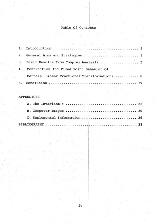
Table Of Conteihts

1. introduction ...

2. General Aims and Strategies ..

3. Basic Results From Complex Ana ysis . 5

4. Contraction And Fixed Point Behavior Of

Certain Linear Fractional Transformations 8

5. Conclusion ... ... 19

APPENDICES

A. The Invariant a ... 22

B. Computer Images ... 30

C. Suplemental Information 36

BIBLIOGRAPHY ... 38

1. IntroduGtion

The purpose of this project is to apply the of

contraction maps on the unit circle in the , to

linear fractional transformations of monomial and

A linear fractional transfoirniation T is a rational

function of the form T(z) = az + where a, b, c.

CZ +

and d are complex numbers and ad - be 0. This restriction

is very essential, for otherwise T"(z) = ad - be = 0 for

( CZ + d)2

all z, so T is identically constant. The function T maps

distinct points onto distinct imagBs. Note also that T has

a pole of order one at - d/c and lim T(z) = a/c . 'Z I

Hence, a linear fractional transformation is a one - to

- one mapping of the complex plane plus the point at ~ onto

itself. Conversely, a one - to - one function (analytic)

mapping of the complex plane plus " onto itself is a linear

fractional transformation. In addition, a linear fractional

transformation that is not identically equal to z has, at

most, two distinct fixed points z for which T(z)= z.

Linear fractional transformatLons are very important in

transfoinnations are :

a) They arei functions that preserve

angles between curves. Hence, they are important tools in

studying flows and fields, and in solving boundary - value

problems, b) Since linear fractional transformations can be

factored into translations, rotations, dilatations, and

reciprocation, ( which are called "simple types" ) these

transformations are extremely important in the study of

geometry, c) Linear fractional treinsformations have a major

role in the study of real one - dimensional projectivities,

since every projectivity can be represented by a linear

fractional transformation,

^incilly,

a

geometrical

characterization of linear fractional transformations is that

they are the only circle preserving transformations in the

2. General Aims And StrateQies

We will prove and make use of two baslG lemmas. The

first one is from complex analysis and is a consequence of

Rouche's Theorem. The second one is a computational lemma

from the theory of linear fractional transformations.

We will use T to denote an arbitrary linear fractional

transformation. The set of all transformation T forms a

group under composition which we \/ill denote by G . It is

well known that G is isomorphic to the projective linear

group over complex numbers.

We will analyze the action of transformations in the

monomial subgroup M of G consistirig of those T with either

a = d= 0orb = c = 0, and of triansformations in the upper

and lower triangular subgroups of G . We denote the upper

and lower triangular subgroups by U and L respectively.

In addition, throughout this text we will let C = -( z :

|z| = 1 } the unit circle, D = { z

IzI < 1 > the open unit

disk. We will be concerned with images of C and D under a

transformation T. By way of definition, we say that T

contracts, or shrinks C provided

T (exp(i6)) I < 1 for all

important properties of these actions:

1) Analyticity on the unit disk,

2) Contraction behavior on the unijt circle,

3) Fixed Point behavior on the unit disk.

The reason for focusincf on the^

that certain surprising conclusions will be reached regarding

the interplay of these three properties. These conclusions

will be stronger than the lemmas W( use for tools, and will

be more specific.

Finally, we note that elements of the group G are

classified up to similarity by a:n invariant known as the

magnitude of T; see[3]. This inviriant determines whether

the transformation T is of Elliptic. Parabolic, Proper

Hyperbolic, Improper Hyperbolic, and Loxodromic type. In

appendix A , we will provide examples of transformations

exhibiting the behaviors we have analyzed in this project

according to the various similarity type. In addition, we

will illustrate some of these c6nclusions using computer

pictures of images of the disk for some examples in Appendix

3. Basic Results From Complex Analysis

Throughout this exposition we: will need certain result

from complex analysis. One of the important results is

Rouche's Theorem, which is as foilows; Suppose f and g are

analytic on an open set containing a piecewise smooth simple

closed curve F and its inside. If

If(z) + g(z) I < |f(z) I for

all z e F, then f and g have an equal number of zeros inside

F, counting multiplicities. ( The proof of this theorem can

be found in any complex variable t ext, such as [2].)

Lemma(1V : Suppose that f is analytic on a domain containing

{ z : |z|

1 }

and that| f(ex]p(i0))|<1

for 0^0:^ 2u.

Then f has exactly one fixed point; in the disk |z|< 1; that

is, if f shrinks C then the equation f(z) = z has precisely

one solution in D .

Proof;

Let g(z) = f(z) - z and h(z) = z. Clearly both g and h

are analytic oh a domain contain ng the closed unit disk.

Further,| g(exp(i0)) + h(exp(i0) 1 = 1 f(exp(i0)) I

1 = 1 h(exp(i0))

|

for all 0, 0 k 6 2ti. Hence, by Rouche's Theorem g and h

point in D counting multiplicities //

(We will refer to Lemma(l) as the fixed point lemma.)

We will also make extensive use of the following

technical lemma which is purely a c:onsequence of the complex

arithmetic of Linear Fractional Transformations.

1

Lemma(2)t A Linear Fractional Transformation T= a b

c d

contracts C iff lap + bp < cp + jdp - 2|cd - ^

Proof;

I T(exp(i0))I =

c(exp(ie)) + and this fraction

is less than one iff |a(exp(i0)) +

b| < |c(exp(i0)) + dj.

Since both sides are non - negativie, this ineqpiality is

equivalent to |a(exp(i0)) + bp <

c(exp(i0)) + dp. Since

jzp = z2/ we have

(5(exp(-10)+B))(a(exp(10)+b)) <

(B(

e3q)(-i0)+d))(c(exp(i0)+d))

which yields

aa+bB+ab(exp(10))+ba(exp(-10)) <

cC+

dd+c<r(exp(10))+dc(exp(10)

and then

I a|2+|bp+ 2Re(aB(exp(i0))) < jcp

+|dp+ 2Re(c3(exp(i0)))

which we can write as

Since only the far right hand term depends on 0 and the

inequa,lity must hold for all 0, the

hold iff the inequality is satisfi^

term achieves its minimiom . HoweiVer, the minimum value of

this term is -2 l ed - a"b|, Therefore, |T(exp(i0))

|< 1 for

all 6 iff |a|2 + |b|2 < |c[2 + jdj2 - 2|cd-aB|. //

(We will refer to Lemma(2) as the contraction lemma.)

In order to demonstrate the usefulness of the

contraction lemma, note that a transformation of the form

4. ContractIbn And Fixed Point Belavlor Of Certain Linear

Fractional Transfc rmations

A. Monomia1 Transformations ; These are transformations in

the subgroup M = { T e Mi _{b = c = 0 or a = d = 0 }.}

Note that the set of transformations T = _{a 0 form a}

0 d

a subgroup of index 2 in M. The other coset consists of

those transformations T = 0 b Thus, it is clear

G 0

why they are called monomial

transformations

♦

They have

either the form T(z) = b

or T(z) = a^z) .

c(z)

Case I. a = d = 0, T(z) = b

/ c(z

If |b| < |c| then

1. T has singularity at the origin.

2. T shrinks C.

3. T has two fixed points insLde D.

1

Example; T(z) =

;

fixed points are ±(l+4i) /

(17)

and property (2) is satisfied by t

If |b| = |c| then

1. T has singularity at the origin.

2. T does not shrink C.

3. T has two fixed points on

Example; T(z) = 1/z ;

fixed pointib are ± 1 which is on the

unit circle and property (2) is satisfied by the contraction

lemma.

If |bl > |c| then

1. T has singularity at the origin.

2. T does not shrink C.

3. T has two fixed points outside D.

Exctmplet T(z) = 7 / 2z ; fixed points are ± (7/2) and

property (2) is satisfied by the contraction lemma.

Case II. b = c = 0, T(z) = a(z)

1. T is analytic in D.

2. T shrinks C iff |a| < |d|

3. T has zero as its only fix:ed point in D.

Example: T{z) = z / (4+i) ;

the u

and by contraction lemma T shrinks C.

Note: The next two follow easily by the contraction lemma,

i) If I a] = ld| we have a pure rotp

Thus, T does not shrink C. ii) If |a| > Idl T does not

shrink C.

B.

Upper Triangular Transfonr^ations

These transformations T = I a b have the form T(z) = az+b.

0 d d

Sometimes they are referred to as integral transformations

I. Suppose a = d, then T(z) = z + b/d. Here we have

transformations of the form T(z) = z + r where.

1. T is analytic in D.

2. T does not shrink C for an

y .r

3. T has no fixed points unless r = 0 , which implies T

eguals the identity function which fixes everything .

Geometrically T is a pure translation which moves the

unit circle to a circle of radius i centered at F = b/d. Let

us use the contraction lemma to give an analytic proof of

property (2).

Proof of property f 2'>:

T(z) = z + r . Assuming F not equal to zero and

applying the contraction lemma tg T , if T shrinks C, we

would have

1 + I F |2 < 1 - 2] -F I

1 F

[2

<

-2] F 1

I F 1

<

-2, a contra

Since F = b/d, F could be any ron-zero complex number .

Thus, T does not shrink C. //

II. Suppose b = d , then T(z) = Fz + 1. Here, as T

= a/d

varies, the images of C under T fo:t:m a family of concentric

circles centered at 1 . In addition,

1. T is analytic in D.

2. T does not shrink C for any P.

3. If r 4= 1/ T has unique fixed point which may or may

not be in the unit disk. If F = this implies , T has no

fixed point.

Proof of property (2)t

T(z) = Fz + 1 once again, assuming F not equal to zero

and applying the contraction lemma to T , if T shrinks C, we

would have

|F|2 +1 < 1-2

l-FI

|F|2 < -2|F|

|F| < -2 , a contradict

Since F = a/d , F could be any illon-zero complex number .

Thus, T does not shrink C. //

Note: This case , b = d and c - 0 , is a counter example to

the converse of fixed point lemma Which is : If T has a

unique fixed point in C and is analytic in D, then T shrinks

C.

•. .V ■

Example: Let F = 3, T(z) - 3z +

1. T is analytic in D.

2. T does not shrink C by contraction lemma.

3. T has unique fixed point in D. Which is -5 .

So far we have looked at spec:ific cases. Now we will

conclude with the general case. That is the case where a, b

and d are possibly distinct .

Ill. Suppose a , b and d are arbiirary. Then T(z) = az + b

: ■ ■■ ■■ ■ ■■: d : ■;

where

1. T is analytic in D.

2. T shrinks C iff |b| < |c

■ 3. T has unique fixed point

in D iff lb| < I d ^ a | .

Proof of property (2) :

Once again by the contraction lemma

lajz + |b|2 < |c|2 + |d|2 - 2|c(

- ab1 . But since c = 0

we have

|a]2 + |b|2 < |d|2 - 2|ab|

|a|2 + 2|a| |b| + |bl2 < |dl2

( I a 1 + IbI )2 < I d|2

since

Ia| + Ibl <

- a

Note: We have actually verified the fixed point lemma for

the case a, b, and d arbitrary and c,= 0, without the use of

Rouche's Theorem. We contrast the following two examples;

Examplefl^ t

T(z) = ((l+i)z + i) / (

5 - Si ) ,

Example(2):

T(z) = (5 - 21)z - i

In both cases, the fixed point 1+i

(-3 + 41) / 25 Is In D. In the first case T shrank C, where

as In the second case T does not shrink C.

C. Lower Triangular Transformations: These are

transformations In the subgroup ]L={TeG:b

= 0}. They

are of the form T(z) = az / (cz ^ d)

we have

1. T has singularity at -d/c .

2. T shrinks C Iff |a|2 < (|d| - |c|)2.

3. T has unique fixed point In D Iff [cj < |a-dl.

We will need to prove propeji

doing so we will show directly. without the use of Rouche's

Theorem , that property (2) Implies property (3) provided T

Is analytic In D.

Proof;

Assume jcl

conclude

< ld| .

. t

From [a

2 < ( jdj - lc|) 2 we can

|a| < |dl - Id

which implies |c| < |d| - |a|

using the Triangle Inequality we get

jcj < |d - aj

Thus, T has unique fixed point in D. //

Now we will prove properties (2) and (3).

Proof of property 12V ;

T(z) =

(az) / (cz + d)}.

Using contraction lemma

directly we get

|a|2 < |c|2 + |d|2 - 2|cd|

|a|2 < ( Id] - lc|)2

Therefore, T shrinks C iff jaj^ j< (jdj - |c|)2. //

Proof of property (3\ ;

T(z) = (az) / (cz+d). Note, for a transformation in

this group, zero will always be a fixed point. So, in order

to find the other fixed point, set T(z) = z. Now we have

(az) / (cz + d)

=

z

az

= cz^ +1 dz

cz2 + (d-a)z = 0

z( cz + (d-a)) = 0

either z = 0 or cz + (d-a) 0. Thus, the other fixed

point is z = (a-d) / c. Therefore, T will have a unique

fixed point in D iff |

a-d| /|

|i

c

implies |c1 < |a-d|

//

Since the transformations in L have singularity at

-d/c, we investigate further to determine the behavior of T

when the pole is inside or outside D. Thus, we observe the

Case I. analytic in D.

By the contraction lemma if T shrinks C then T has

unique fixed point in D.

T(z) = ' iz ■

z + 7

By the contraction lemma T shrinks C and T has two

fixed points, 0 and -3, where 0 is the unique fixed point in

D. (see t B, Fig. 1, for ii

On the other hand, if T does not shrink C, T may or may

not have unique fixed point in D. Example; T(z) = lOz

z + 6

By the contraction lemma T does not shrink C , and T

has two fixed points, 0 and 4, where 0 is the unique fixed

point in D.

Example; T(z) = 3z

z + 3

Once again by the contractioii lemma T does not shrink

C, and T has a fixed point of multiplicity two at the

origin.

Note: The case where T shrinks C and T has no unique fixed

point cannot occur since property (2) implies property (3).

Case II. jcj > |d| singularity inside D.

By contrast with case I, if T shrinks C it will

necessarily has two fixed points in D. We see this as

follows:

Proof:

If zero was the only fixed [point in D we would have

|c| < la-d|

which is

^ I a I + 1 d I .

But then

|cl - |di < |al

which is equivalent to

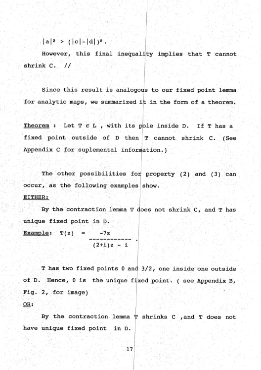
|a|2 > (lc|-ldl)2.

However, this final inequality implies that T cannot

shrink C. //

Since this result is ahalogous to our fixed point lemma

for analytic maps, we siuraaarized it in the form of a theorem.

Theorem : Let T e L , with its pole inside D. If T has a

fixed point outside of D then T cannot shrink C. (See

Appendix C for suplemental information.)

The other possibilities for property (2) and (3) can

occur, as the following examples show.

EITHER:

By the contraction lemma T does not shrink C, and T has

unique fixed point in D.

Example: T(z) = -7z

z - i

T has two fixed points 0 and 3/2, one inside one outside

of D. Hence, 0 is the unique fixed point. ( see Appendix B,

Fig. 2, for i:

OR: ,

By the contraction lemma T shrinks C ,and T does not

have unique fixed point in D.

Example: T(z) = iz

^^^«mm^mmt mmm mmi% mmm^mmm mmm ^

7z + (2+i)

T has two fixed points 0 and -2/7. Hence, both fixed

points are inside D. (see Appendjix B, fig. 3, for image)

OR;

The following examples show the question of

multiplicity is crucial for property (3)•

By the contraction lemma T shrinks C, and T does not

have unique fixed point in D.

Example: T(z) = z

4z + 1

T has a fixed point of multiplicity two at the origin.

OR:

By the contraction lemma T does not shrink C, and T does

not have unique fixed point in D.

Example: T(z) - 2z

3z+2

T has a fixed point of multiplicity two at the origin.

5. Conclusion

In conclusion , we have used linear fractional

transfbmations monomial and triangular types as explication

of the fixed point and contraction lemmas from complex

analysis. However, we have seen some surprising situations

and have cited examples for these situations. In short

siommarizing the different classes we have the following:

I. In the class of the monomial transformations we

observed that EITHER T had singularity at the origin where T

a) shrank C and had two fixed poiints in D, b) did not shrink

C and had two fixed points in D, c) did not shrink C and the

two fixed points were outside D; OR T was analytic in C

where T a) shrank C and had unique fixed point in D, b) did

not shrink G and had no unique fixed point in D. Hence, a

pure rotation. Thus, part a) of the latter conclusion showed

that this was the only situation where the fixed point lemma

could be satisfied under this class.

II. In the class of the upper triangular

transformations we obseirved that : T was analytic in D where

T a) did not shrink C for any V and had no fixed point in D,

did not shrink C for any F and had unique fixed point

which may or may not be in D. Notice, this situation implies

that: the converse of the fixed point lemnia will not hold.

(Surprising!!) c) did shrink C iff |b| < |d| - jaj and has

unique fixed point iff |b| < Id - a I . Notice this

conclusion proves the fixed point lemma without Rpuch©'s

Theorem. This is another surprising outcome!!

III. in the class the lower triangular

transfoiPnations we observed that:

a) T had singularity at: ­

d/c, b) T shrank C iff jaj^ < ([d|

I - IcI )2, c) T had unique

fixed point in D iff |c[ < ja -

were disjoint from one another.|( This was an interesting

conclusion ! )

Due to the singularity at -d/c we were curious to find

out about the behavior of T wh

k

outside of D. Thus, after several investigations we coneluded

that EITHER : T was analytic in D where T a) shrank C and had unique fixed point in D, b) did not shrink C and had

unique fixed point in D. OR: T had singularity inside D

where T a) did not shrink C and had the origin as its unique

fixed point in D, b) shrank C and had two fixed points inside

D/ c) did shrink C and had a fixed point of multiplicity two

at the origin d) did not shrink C and had a fixed point of

multiplicity two at the origin.

Thus, as a result of these surprising outcomes for this

class, we were able to summarize our observations in a

theorem.

Theorem : Let T e L with its pole inside of D. If T has a Le insi(

fixed point outside of D then T can not shrink C.

ADPendix A

I

We have investigated the majner in which the monomial

and triangular type linear fracticlnal transformations behave

with respect to the three properties. That is ; 1)

analyticity on the unit disk, 2) contraction behavior on the

unit circle, 3) fixed point behavior on the unit disk. We

shall now study, using tables, their similarity invariant defined by ; o = (tr T)^

- 4 where T = a b

c d

T T T

o is sometimes called the magnitude of the linear fractional

transformation. Note that it can be shown that two linear

fractional transfoinaations are similar in the group G iff

their magnitudes are equal. See [3]

The transfoimiations T are classilfied as:

Parabolic { which is similar to a translation } if o = 0 ,

Elliptic { similar to a rotation} if -4 ^ o < 0,

Proper Hyperbolic {similar to a dilatation} if o > 0,

Improper Hyperbolic {similar to a dilatation} if o ^ -4 ,

Loxodromic {leaves ho circle invariant} if o is not real. Once again, [3] describes this choice of terminology in

terms of invariant pencils of circles in the Moebius plane.

Note: for the triangular type we nave either

T = a b or T = a 0

0 d c d

Note that, a = (a + d)2

4 in both cases.

;■ ad

For the monomial type there is the additional

possibility

T = 0 b in which case o ^ -4 c 0

In this appendix we will indicate whether or not a

transformation of a particular type can exhibit the

properties (1), (2), and (3), which we have analyzed in this

paper. For example: if we were considering T e M then we

will find neither Parabolic nor Proper Hyperbolic nor

Loxodromic transformations which are analytic in D. In this

case there are no transformatioins of these type in M. We

will indicate this in the table by the word NP to imply not

possible. On the other hand M contains Improper Hyperbolic

trans formations However, they are singular at the origin.

We will indicate this in the table by the word No.

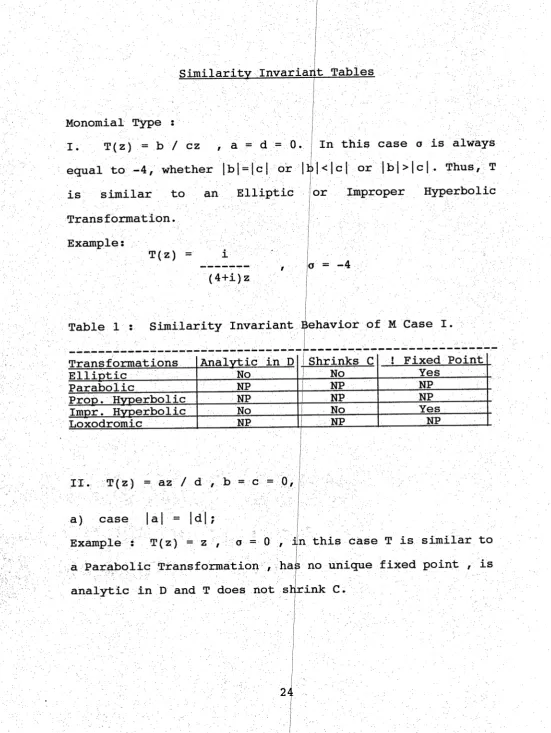
SvTni-laritv Invariar[t Tables

Monomial Ti^e :

I.

T(z) - b / cz , a - d = 0. In this case a is always

equal to -4, whether lbl=|cl or lb|<|c| or lbl>lc|. Thus, T

Elliptic

or Improper

Hyperbolic

is similar to an

Transformation.

T(z) =

o = -4

Table 1 : Similarity Invariant Behavior of M Case I.

Shrinks C I Fixed Point Transformations Analvtic in D

Yes

Elliptic No 1 No

Parabolic NP NP NP

Prop. Hvperbolic NP NP NP

No Yes

Impr. Hvperbolic No

lioxodromic NP NP NP

II.

z) = az / d f b = c = 0,

a) case [a] = ]d|;

Example : T(z) = z ,

50 - 0 , in this case T is similar to

a Parabolic Transformation , has no unique fixed point , is

b) case |a| < |b| ;

In this case T could either ibe similar to a Proper

Hyperbolic Transformation, which! implies that o > 0,

Example : T(z) = (2i)z / 5i , p = 0.9 .

or T could be similar to an Improper Hyperbolic

Transformation . This implies that o -4 ,

Example : T(z) = (3i)z/ -4i , o -4.01 .

or T could be similar to a Loxodromic Transformation

This implies that a is not real.

Example : T(z) = z / (4+i) , o ^ (26 - 32i) / 15 .

Table 2 : Similarity Invariant Behavior Of M Case II (b)

Transformations Analvtic in B Shrinks C ! Fixed Point

Elliptic NP NP NP

Parabolic NP NP NP

Prop. Hyperbolic Yes Yes Yes

Imp. Hvperbolic Yes 1 Yes Yes

Loxodromic Yes 1 Yes Yes

upper Triancnilar Transformations

T(z) = (az + b) / d }

I. If a = d then o = 0 , which implies that T is

Similar to a Parabolic Transformation.

z) = z + 3 .

il. If b ¥ d then either 0, which implies that T

is similar to a Proper Hyperbolic

: T(z) = 4z / 5 1 / o =

or o -4 , which implies that T is similar to

an Improper Hyperbolic Transformation,

Example : T(z) = (7z - 2) / -2 / a = -5.79

or o is not real , which implies that T is

similar to a Loxodromic Transformation.

Example : T(z) = (4z + i) / i , j o = (32 + 60i) / -16

Table 3: Similarity Invariant Behavior Of U Case (II)

Transfomations Analytic in D Shrinks C ! Fixed Point

Elliptic NP NP NP

Parabolic Yes No No

Proper Hvperbolic Yes Yes No

Impr. Hvperbolic Yes i Yes No

Loxodromic Yes i Yes No

Ill. If a , b , and d are distinct then either a > 0,

which implies that T is similar to a Proper Hyperbolic

Transformation,

Example : T(z) = (z + 2) / 7> o |= 5.1 .

or o ^ -4f which implies T is similar to an Improper

Hyperbolic Transformation,

: T(z) = (

7z - 2 ) / -2 , o = -5.79 .

or a is not real, which implies that T is similar to a

Loxodromic Transformation.

+ i)z + i) / (5 - 2i), a = (49-21i)/58

Table 4: Similarity Invariant Behavior Of U Case(III).

Transformations Analytic in D Shrinks C 1 Fixed Point

NP NP NP

Parabolic NP NP NP

Proper Hyperbolic Yes Yes Yes

Impro. Hyperbolic Yes Yes Yes

Loxodromic Yes Yes Yes

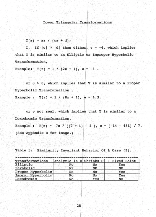
Lower Triancmlar Tramsforiaa1:ions

■

: T(z) = az^7 (cz + d);

I. If ]cI > Id] fcheil either, a =

that T is similar to an Elliptic pr

Transformation,

: T(z) - 1 / (2z + 1), o = -4 .

or o > 0, which implies that T is similar to a Proper

Hyperbolic Transformation ,

: T(z) = 3 / (8z + 1), p = 4.3.

or o not real, which implies that T is similar to a

Loxodromic Transformation.

Example : T(z) = -7z /

((2 + i)

= (-14 - 48i) / 7

(See Appendix B for image.)

Table 5; Similarity Invariant :Behavior Of L Case (I).

Transformations Analytic in D Shrinks C ! Fixed Point

Elliptic ■ ■ ^ No No Yes

Parabolic NP . NP , ^ NP

Proper Hvperbolic No No ■ Yes ■

Impro; Hvperbo1ic No NO Yes ■ ■ ■■

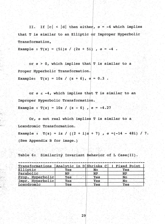
II. If IcI < IdI then either, o = -4 which implies

that T is similar to an Elliptic or Improper Hyperbolic

Transfomation,

Excimple : T(z) = (5i)z / (2z + 5i) , o = -4 .

or o > 0, which implies that T is similar to a

Proper Hyperbolic Transformation.

T(z) = lOz / (z + 6), a = 0.3 .

or o ^ -4, which implies that T is similar to an

Improper Hyperbolic Transformation.

: T(z) = lOz / (z - 6) , a = -4.27

■

Or, a not real which implies T is similar to a

Loxodromic Transformation.

Example : T(z) = iz / ((2 + i)z + 7) , o =(-14 - 48i) / 7.

(See Appendix B for image.)

Table 6: Similarity Invariant Behavior of L Case(II)

Transformations Analvtic in D Shrinks C ! Fixed Point

Elliptic : Yes No • Yes

Parabolic ■ NP NP • NP ■

ProD. Hvoerbolic • ■ ■Yes'^ ' ■i'"'"­ Yes -No^

Impr. Hvperbolic ■■ Yes Yes No

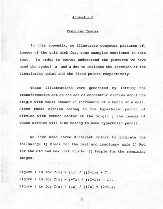
* Appendix B

Computer Images

In this appendix, we illustrate computer pictures of, images of the unit disk for, some examples mentioned in this

text. In order to better understand the pictures we have

used the symbol x and a dot to indicate the location of the

singularity point and the fixed points respectively.

These illustrations were generated by letting the

transformation act on the set of concentric circles about the

origin with radii chosen in increments of a tenth of a unit.

Since these circles belong to the hyperbolic pencil of

circles with common center at the origin ,

the images of

these circles will also belong to some hyperbolic pencil.

We have used three different colors to indicate the

following: 1) Black for the real and imaginary axis 2) Red

for the old and new unit circle 3) Purple for the remaining

images.

Figure 1 is for T(z) = (iz) / ((2+i)z +7).

Figure 2 is for T(z) = (-7z) / ((2+i)z - i).

Figure 3 is for T(z) = (iz) / ((7z) + (2+i)).

Figure 4 is for T(z) = (3z) / ( 2z +1).Although this

exaiaple is not mentioned in this t€Jxt, we wanted to include

it^ i.n order to demonstrate the im(age of the disk when tke

fixed point is on the unit circle.

fig. 1

.y­

/I, «fi' "

• ■r

\:i

yy^y

Uh

; ■ . ,/■ V''#i

f-I#

Py

.

• =

\

/. ,

H­

fig. 3

» ■ : ■■■■• . •■■ ^ -,■ • ..r - ■••■■■^^ - v. ,

%-f' > - i ■ ' - "t, ■ ; "' _{■•;' W ■ <}

• ■ "• ••

' "

G

fig. 4

e R R AT U M

Page 36, Appendix: G Lemma (3) smould read as follows;

Lemma (3) r The group of automorphisms of the unit

disk ca,n be factored into the grcup of rotations about

the origin and the groub of trandlformations of the form

1 -a

Appendix G

Supplemental Information

Theorem ; Let T e L, with its polel inside D. If T has a

fixed point putside of D then T canno^ shriiik C.

Note; This theorem is in fact true for etny, linear

fractional transformation . That is, given any linear

fractional transformation T, whose pole is in D and has

fijced point outside D, T cannot shrLok C.

; The proof of

note requires

the two lemmas used in this paper . But we note that it

involves only one additional lemma which is proved in most

standard text about linear factional transformations.

Lemma(3) : The group of automorphismp of the unit disk can

not be factored into the group of rotations about the

origin and the group of transformatipns of the form

1 -a -JT 1

with a < 1.

Using lemma(3) we can extend the above theorem as

follows: First note that if d = 0 in our transformation

then we can assume that |c - 1 . Thus the transformation

T(z) 4= a + b/z has singularity at th<

to see that if T has a fixed point outside of D then T

cannot shrink the unit dircle. On the Other hand if

d = 0 but the pole is inside the disk then we can compose

with an automorpism of D and reduce to the case where the

pole is at the origin we will not lose any generality by doing this since the automorphism in lemma(3) leaves the

outside of D invariant.

MM

. ■(:

■ ■" '

, ■ ■ r ■

BIBLIOGRAPHY

1) Burn, R.P., Groups; a path to geemetrv . Great Britain,

1987; rpt. in Great Britair^

Cambridge, 1988

2) Fisher, Stephen D., Complex Variables. 2nd ed.

Belmont, CA. Wadsworth, 1986.

3) Schwerdtfeger, Hans. Geometiry Of Complex Numbers

New York: Dover Publications, 1979.