RESEARCHARTICLE
An algorithm for the selection of
route dependent orientation
information
Heinrich Löwen and Angela Schwering
Institute for Geoinformatics, University of Münster, Germany
Received: July 15, 2019; returned: October 16, 2019; revised: November 30, 2019; accepted: March 16, 2020.
Abstract:Landmarks are important features of spatial cognition and are naturally included in human route descriptions. In the past algorithms were developed to select the most salient landmarks at decision points and automatically incorporate them in route instruc-tions. Moreover, it was shown that human route descriptions contain a significant amount of orientation information, which support the users to orient themselves regarding known environmental information, and it was shown that orientation information support the acquisition of survey knowledge. Thus, there is a need to extend the landmarks selec-tion to automatically select orientaselec-tion informaselec-tion. In this work, we present an algorithm for the computational selection of route dependent orientation information, which extends previous algorithms and includes a salience calculation of orientation information for any location along the route. We implemented the algorithm and demonstrate the functionality based on OpenStreetMap data.
Keywords: orientation information, algorithm, navigation, wayfinding support, land-marks, survey knowledge
1
Introduction
locations along the route. While the broad availability of these systems fundamentally changed peoples’ wayfinding behavior, it was shown that this has negative consequences on human spatial abilities [5, 21, 31, 41]. During car navigation, people tend to blindly follow the instructions of the navigation devices without active engagement with the en-vironment, which makes them unable to orient themselves even after recurrent drives [4]. However, recent research has shown that the accentuation of orientation information has a significant effect on peoples’ spatial knowledge acquisition during wayfinding. When people are presented with global and structuring information during navigation, this infor-mation is automatically learned, which leads to a positive effect on peoples’ survey knowl-edge [37].
Previous research proposed computational methods to identify the most salient land-marks at decision points and presented approaches to automatically incorporate these landmarks in routing instructions. However, the proposed solutions ignore the importance of context and are restricted to the selection of point-like landmarks at decision points. There is the need for an algorithm to automatically select the most salient environmental features for any location along a route and different contexts, e.g., conveying orientation in the local or global context. Orientation information, which includes local and global landmarks and even structuring features, like environmental regions, supports people to orient themselves in the current context. In this paper, we present an algorithm to se-lect orientation information candidates from spatial databases and calculate the salience of these candidates for the current route context (Section 4). While this aligns with research that investigates means to better support survey knowledge acquisition and evaluates the conceptual perspective (e.g., [4, 37, 40]), this work aims to develop a computational method for automatically selecting route dependent orientation information. The solution might be used as a basis for future empirical research. Moreover, we discuss how the algorithm can be modified and implemented into navigation support systems. Although similar methods and solutions might be applicable for different modes of travel, we focus on car navigation and do not concern ourselves with the specifics other modes of travel such as pedestrian navigation. As proof of concept, we implement the algorithm and demonstrate the selec-tion and salience calculaselec-tion based on OpenStreetMap (OSM) data (Secselec-tion 5). We review and discuss the results in the light of the extendability and generalizability of the algorithm (Section 5.2).
2
Related works
2.1
Algorithms for the salience calculation of landmarks
andstructural salienceto assess the overall salience of a landmark. For the visual salience, they considered thefacade area, theshape, thecolor, and thevisibilityof objects and calculate the prominence of the objects in terms of these metrics. With these metrics, they focus on buildings and point-like landmarks, which, however, would not apply to areal landmarks or regions. For the semantic salience, they evaluated thecultural and historic importanceas well asexplicit marksthat specify the semantics of the object. For the structural salience, Raubal and Winter [46] assessed the importance of the location of the landmarks with re-spect tonodes, i.e., the degree of intersection and category of connecting edges, and bound-aries, i.e., objects that separate the street networks. The main shortcoming of this work is the independence of the route; the salience of landmarks is only assessed for separate locations, i.e., intersections, and only local landmarks in the immediate surrounding are considered. Moreover, the solution is not transferable to different feature types like areal landmarks or regional structures.
Winter [59] extended Raubal and Winters [46] measures with the advance visibility, which calculates the visibility of landmarks for a person approaching a decision point. They showed that this measure improves the suitability of the selected landmarks. Simi-larly, Caduff and Timpf [6] presented a framework for the assessment of landmarks salience in the visual field. They proposed that the landmarks salience is based on the trilateral rela-tionship between observer, environment and geographic object. They evaluate the overall salience of visual landmarks in terms of (i) theirperceptual salience, which is based on the visual sensory input, (ii) thecognitive salience, which is based on the prior knowledge of the individual, and (iii) thecontextual salience, which is based on the amount of attentional resources in the visual field. While the visual salience of features is an important aspect for navigation support, the structural salience of environmental features can be considered as more important for supporting orientation [24]. This, however, was only marginally con-sidered in the presented approaches. More follow up research was presented by Klippel and Winter [30], Claramunt and Winter [7], and Quesnot and Roche [44]. Klippel and Winter, and Claramunt and Winter investigated the structural salience of environmental features. Klippel and Winter presented a taxonomy of point-like landmarks with respect to their position along the route, extending the wayfinding choremes theory [29, 30]. Clara-munt and Winter described a generic model of structural salience of environmental features in route directions, which is based on network analysis and space syntax measures [7, 19]. Quesnot and Roche presented a measure ofsemantic salienceof landmarks based on volun-teered geographic information [44].
streetwith respect to the decision points (features that lie on the same side as the turn are weighted higher); in casemultiple landmarksof the same category are in the candidate set, only the first instance of the category will get the full weight, whereas the others are dis-missed. Rousell and Zipf [48] presented an approach to automatically extract landmarks for pedestrian navigation from the OSM database. Their method is based on a number of metrics that are used to assess the overall salience of landmark candidates at decision points. In line with Duckham et al. [12], they specifyfeature category weightsand consider thelocationof the features in relation to the direction of travel (opposite side, same side). Similar to the multiple landmarks metric of Duckham et al. [12], they specify the unique-nessof features, i.e., if multiple features of a category are in the candidates set, all features get reduced weights. Additionally they present metrics for thevisibility, thepositionof the feature in relation to the decision point (before, alongside, after), and thedistance. Besides the selection and salience calculation of environmental features, approaches for including landmarks and other contextual information in route directions were presented. Klippel et al. developed different data structures for cognitive ergonomic route directions [17, 26] and presented approaches for chunking route instructions [28]. Klippel et al. described different chunking types, which, however, mainly aim to improve the navigation support, e.g., numerical chunking and landmark chunking. Only structure chunking might be rel-evant for the current work, however, the authors did not present an algorithm for this type of chunking. Other approaches considered the prior knowledge of the navigator and developed formal models for generating personalized route instructions [43, 49, 57].
While the presented approaches are useful for enriching wayfinding instructions with local landmarks, the main shortcoming that was not considered over the years is the lim-itation to the features selection at intersections and decision points. It was shown that landmarks are not only important locally at decision points, but also along the route and even globally when distant to the route [1, 33, 34, 55]. The visual salience of landmarks at decision points is an important factor for navigation support, however, structural salience might be the more important factor when calculating the salience for orientation support. Moreover, it is criticized that current approaches focus on point-like landmarks, neglecting regional landmarks or structural regions [35, 51]. In the existing approaches, regions were, if at all, only considered conceptually, however, no algorithms were presented to calculate the salience for regional landmarks or structural regions. Sester and Dalyot [52] pointed out that, besides local route information, information should be provided, which embeds the route in the global context; Löwen et al. [37] showed that besides landmarks, struc-tural regions are important features in human wayfinding. This orientation information was shown to support the acquisition of survey knowledge [37]. There is a need for an algorithm to automatically select the most salient orientation information; moreover, the algorithm should not be restricted to the selection of local features at decision points but it should automatically select orientation information for any location and context along the route.
2.2
Orientation information in context
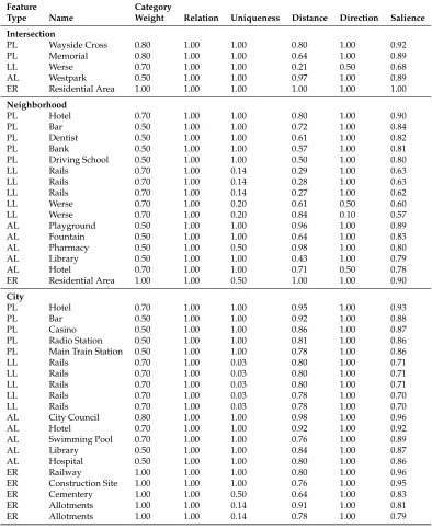
orientation information, the location is not fixed, but changing with regard to the users’ drive along the route. Thus, the location is one important contextual parameter. Addition-ally, orientation is related to ascale relevant to the current goal. In previous work, a classifica-tion scheme offunctional scalesin assisted wayfinding was developed, where a conceptual distinction of scales with respect to different goals in assisted wayfinding scenarios was proposed [36]. Maps at different scales might target different tasks such as supporting the identification of a decision point or providing an overview of the local or global route context. The functional scales are distinguished with respect to their role in supporting wayfinding and orientation and the containment of features relevant for different aspects of navigation [36]. The authors distinguish the scalesintersection, neighborhood, city, region, androute overview. While theintersectionscale depicts the decision point at a large scale and requires detailed information about the decision point, the map scales of theneighborhood, city,andregionscale are described to be relative to the size of the particular environment (neighborhood, city, region) and maps should depict information for supporting the un-derstanding of these environments. Theroute overviewscale combines information of the previous scales to support the understanding of the global route context. Consequently, en-vironmental features that are depicted in the particular maps need to be selected to support the task in the best possible way. For the scope of this paper, we consider the functional scales as a second important contextual parameter, which defines the relevant size of the environment and the representation of the map.
Functional scale Information content Function in wayfinding support Related cartographic scale Related psychological scale
intersection – detailed information about DP – building information – local landmarks – full street network
– identification of DP – local orientation – understanding of visual information at DP
fixed large scale * vista space
neighborhood – information about local context – local & global landmarks – full street network – structural regions≤
neighborhood
– understanding of local route context
– understanding of surrounding connections
relative to size of neighborhood
environmental space
city – information about global context of city
– global landmarks – main street network – structural regions≤city
– understanding of global city context
– understanding of city structure and main connections
relative to size of city **
environmental space
region – information about global context of the region
– main street network – structural regions≥city
– understanding global region context
– understanding of main connections through region
relative to size of cities and regions
geographical space
route overview
– combined information from neighborhood, city and region scale
– understanding of the global route context
– getting overview of whole route
relative to length of route
* E.g., for an average 5 inch smartphone screen this relates to a map scale of 1:1.000–1:3000. ** E.g., for the city of Münster, western Germany, this relates to a map scale of 1:100.000–1:200.000.
Table 1: Functional scales in wayfinding support (reproduced from Löwen et al. [36]).
only. We parameterize the salience function to the context, i.e., the current location along the route and the target scale.
3
Theory
Landmarks were shown to be important features in human wayfinding and key features in spatial cognition. Although landmarks are defined to be any geographic object that struc-tures human mental spatial representation [47], landmarks are dominantly considered as point-like objects such as a specific building. Because of their importance to structure hu-man mental spatial representation, landmarks are often used in huhu-man communication. It was shown that people include local landmarks at decision points and along the route, as well as global landmarks off-route [8, 9, 33, 34, 39, 55, 56, 60]. Anacta et al. [3] presented em-pirical evidence that human wayfinding instructions contain a significant amount of orien-tation information, i.e., information that supports people to derive their position in space and orient themselves with regard to known environmental information [32]. We previ-ously developed a classification scheme of orientation information that specifies feature types and features roles in route maps [36]. The feature typeslandmarks,network structures andstructural regionsare distinguished, moreover, the role features might take with regard to the route, i.e., local or global, is specified [36].
Landmarkscan be any point-like, linear, or areal object in the environment and may be relevant in the local or global context of a route.Network structuresare defined as the rele-vant street network to be selected for orientation support. This might be on the one hand thenetwork skeletonconstituting the overall structure of the street network (global context) and on the other hand the route relevant network including side streets and detailed net-work related to the route (local context). Structural regionscompriseadministrative regions andenvironmental regions, which are relevant for the global context of the route. They were shown to support incidental spatial learning of survey information when included in route descriptions [37]. Whereas areal landmarks are separate geographic objects with an areal extent, structural regions are in contrast defined by theirbona fideorvagueboundaries (en-vironmental regions), orfiatboundaries (administrative regions) [15,53], which might have containment relations with other features. Environmental regions have a semantic mean-ing, which refers to some kind of homogeneous and perceivable environmental structure, such as urban vs. rural areas or a city center. Administrative regions might only be per-ceivable in the environment through signage or external reference. The example of a city might be considered twofold: on the one hand, a city has a clearly defined administrative boundary, which is apparent via signage; on the other hand, and not necessarily corre-sponding, a city might be considered as the build area in contrast to the surrounding rural area. Structural regions are rarely incorporated in current navigation systems; however, they can be useful features for supporting orientation by helping users to structure their mental spatial representations [36].
spatial databases do not exist. Moreover, the perception of regions and region boundaries is strongly tight to human perception and cognition, which might not coincide with the results of the computational models. Tomko and Winter [58] analyzed the functional rela-tionships between elements of the city in order to model the spatial knowledge of wayfind-ers. In this line, novel methods for detecting regions from spatial databases for wayfinding purposes would be required. The algorithm that is presented here assumes a candidate selection based on the theoretical concept of structural regions, as it was described above. In Section 5.1 we demonstrate and discuss the selection of structural regions from OSM. The candidate set will be refined with respect to the salience in a particular context, which we elaborate in the following section.
While we focused on cognitive aspects for orientation support and spatial learning in previous work, in this work we focus on the computational aspects to automatically select orientation information. Therefore, we adhere to the classification scheme of orientation information and present a selection workflow that consists of two main steps: in a first step general orientation information candidates are selected within a reasonable distance buffer around the route; in a second step the candidate set is refined with respect to the context, i.e., locational and scale context. Different communication modes for wayfinding support exist, however, for the proof of concepts we focus on the visual representation of orientation information on wayfinding maps.
4
Algorithm
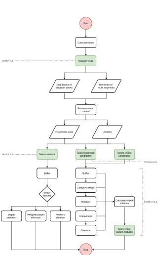
We implemented the following workflow to select orientation information for the visual-ization in orientation maps; we stepwise add information to the selection (see Figure 1). As described above, the relevance of environmental features for orientation support depends on the users’ context in terms of the location and the scale. We initiallyanalyze the route to better define the route context. We analyze the route in terms of the type of streets, the distribution of decision points, and the functional scales (Section 4.1). We thenselect the relevant street networkfor supporting orientation (Section 4.2). Current navigation systems only reduce the level of detail of the represented features with decreasing map scales. We expect that a selection and an accentuation of the main street network will help users to structure their mental spatial representations of space. Thus, in Section 4.2 we elaborate a context-dependent selection of the street network. Finally, weselect landmarks and structural regionsto embed the route into the context (Section 4.3). Therefore, feature candidates are selected from spatial databases (Section 4.3.1), which are then refined with respect to the salience metrics that will be described in Section 4.3.2.
4.1
Route analysis
types are disregarded in the current work. The street types are hierarchically ordered as shown in Table 2 (lower values represent a higher order in the hierarchy).
Value Type 10 highway 20 primary road 30 secondary road 40 tertiary road 50 residential road
Table 2: Types of street segments (T).
DP class DP class description 0 start/destination 1 straight on
2 turn not at a junction 3 turn at a t-junction 4 turn at a junction 5 turn at a roundabout 6 highway ramp/exit
Table 3: Decision point classes (DP C).
The route is analyzed in terms of the hierarchy of the route segments, and the location and distribution of decision points along the route. Routes often have a typical structure with respect to the type of route segments, i.e., increasing hierarchy at the initial part of the route and decreasing hierarchy at the final part of the route [61]. The route structure is utilized for the further selection and embedding of the route in its spatial context. Some of the above-mentioned metrics consider the route structure in the route computation, e.g., natural roads [23] consider the Space Syntax theory [19].
The street network is represented as a graphG = (V, E)consisting of a set of vertices (V) and edges (E), and a route as a directed graphG0 = (V0, E0) ⊆ Gfrom starts ∈ V to destinationt ∈ V. Each edgee∈ Eis defined by two incident verticesx, y∈ V. Each route consists of a set of decision points DP ⊆ V0. Decision points are defined by a set DP Cof decision point classes (see Table 3), represented by a functionclass:DP →DP C, such that for allv ∈DP, class(v) =c,withc ∈DP C. Street types are defined by a setT, represented by a functiontype:E→T, such that for alle∈E, type(e) =t, witht∈T (see Table 2).
Table 3 presents the decision point classes that are used for the analysis of decision points along the route; these were presented in previous work [2]. Straight onclassifies decision points where the route continues straight but intersects street segments of the same or higher hierarchy class. Turn not at a junctionclassifies only vertices v ∈ V0 with degree(v) = 2that require a turn, i.e., there are no side streets but the angle of connect-ing edges exceeds a predefined threshold. Highway ramp/exitspecifically classifies vertices v ∈ V0 of highways, i. e., ramps, exits, connections; thustype(e) = 10withe ∈ E0 ande incident tov. The distribution of decision points along the route as well as the reference segments are used for a further selection of environmental features. Reference segmentsare considered as route segments before and after a particular decision point. They may either be calculated based on a predefined static distance, or a variable distance based on the decision point class, the functional scale, etc. Here, we calculated the reference segments with a predefined static distance of 100 meters.
4.2
Network structures
network including side streets and detailed network related to the route (local context) [37]. For the analysis and the selection of the relevant street network, we define the following functions:
• connected(x, y)tests if edgesx∈Eandy∈Epoint to the same vertexv∈V. • weight_connected(x, y)tests if connected(x, y)andweight(x) ≥ weight(y). For the
weight(), any numeric attribute ofxandycan be chosen; e. g., the route type (hierar-chy) of the edge (see Table 2).
• depth(x)calculates the fewest number of connections of edgexto any edgee∈E0of the route.
• weight_depth(x)calculates the fewest number of connections of edgexto any edge e∈E0withweight(x)≥weight(e).
With these functions, the forthcoming operations can be performed. Based on the specific route context, different parts of the adjacent route network will be considered as relevant and will be automatically selected.
Buffer The surrounding street network is reduced with respect to the users’ context, i.e., the network is reduced to a bufferB around the current locationl ∈ L with a maximal distanceM Df, depending on the functional scalef.
Depth The depth metric selects all adjacent street segments to the route up to a pre-defined depth. This is also referred to astopological distance towards the route. The set Dn is the set of edgese ∈ E, for which depth(e) = n. Thus,P
n
i=1Di is the sum of the selected network up to the maximum depthn. Depending on the functional scale, the adjacent street network is refined with respect to a specified depth.
Weighted depth Similarly, it might be necessary to select adjacent street segments of the same or higherweightwith respect to the connecting route segment, i.e., weighted depth. When driving on a primary road, side streets of a lower hierarchy would for example not be considered as relevant, whereas intersections with streets of the same or higher hierarchy are relevant to be selected. Consequently, the setW Dn represents the set of edgese ∈E, for whichweight_depth(e) =n.
4.3
Landmarks and structural regions
4.3.1 Candidate selection
As mentioned above, first, feature candidates for landmarks and structural regions are selected from spatial databases. In a second step, the candidates will be refined with respect to the salience metrics that will be described in Section 4.3.2.
In spatial databases, individual features are usually attributed to different feature cat-egories, such as shops, parks, etc. For the candidate selection, relevant feature categories need to be specified considering the data structure of the selected spatial database. This is in line with previous research (e.g., [12, 48]). Previous work also considered human subject ratings of separate feature instances as a source for salience calculation [43, 44], however, the authors already pointed out the limitation with respect to the availability and scalabil-ity of datasources, especially when considering the personal dimension of feature salience; thus human subject ratings may only indirectly incorporated through the category weights in the current approach. All features of the specified categories that lie within a reasonable distance to the route, are considered as feature candidates. When selecting landmarks from spatial databases, the candidate set might include a large set of landmarks, thus the main requirement is to calculate the salience of separate landmark candidates.
4.3.2 Core selection metrics
In the previous section, we described the general selection of orientation information candi-dates from spatial databases, regardless of their relevance and salience for a specific context within a wayfinding scenario. The selection of environmental features needs to be refined with respect to their salience for a specific context, i. e., the users’ location along the route and a specific functional scalef ∈Fat which the orientation information will be presented. We define the salience functionSf for a weighing of the candidate setCSwith respect to their salience at the functional scalef ∈ F. In the following, we describe the core set of metrics that are used for the overall salience weighting. These metrics relate to the clas-sification ofvisual, semantic,andstructuralsalience of environmental features [46, 54]. The presented metrics are functions that depend on the route context, i.e., the location and the functional scale, and are applied to the candidate sets of structural regions as well as land-marks. The metrics are not exhaustive, but additional metrics can be developed and added to the overall salience functionSf. In Section 5.2.2 we discuss a few possible extensions of the salience function.
Buffer Depending on the context, only a limited area around the current location along the route will be relevant, which relates to the area of the map that will be shown on the map during wayfinding and navigation. Thus, we refine the candidate set to a buffer around the current location l ∈ L with a maximal distanceM Df. The buffer distance depends on the functional scalef ∈F, which has to be specified for the specific use case. The buffer metric is calculated as
Bf =
1, for dist(l, c)≤M Df
0, for dist(l, c)> M Df
Category weights The salience of different feature categories might differ with respect to the suitability for orientation support, thus category weights might be assigned to the feature categories of the candidate set, such thatweight : C → [0,1](see [12, 48]). C is a set of categories, such that for everyc ∈ C,weight(c)is the normalized salience of that category, withweight(c) = 1most salient andweight(c) = 0least salient. The category weight might vary with respect to the functional scales, such that
Scf =weight(cf)
is considered as the salience of any candidate of categoryc ∈ C at the functional scale f ∈F.
Relation In addition to the salience of the feature category, we specify the relation of a candidate towards the route. The salience of a candidate might be considered as higher when located at decision points compared to features located along the route. Thus, we weight candidates with respect to their relation to the route. We identify for everyc∈CS the nearest point on the route. We considercas locatedat decision point, if the nearest point on the route intersects with the reference segment of the decision point (see Section 4.1). The relation metricRis calculated regardless of the functional scale:
R=
1, for cat decision point
0.5, for calong the route
Uniqueness If several features of the same category exist within the candidate set, the identification of a particular feature in the environment is more difficult. We, therefore, determine the uniqueness of the features within the candidate set (see [48]). The uniqueness is calculated by
Uc = 1/nc
whereUcis the uniqueness of a feature of categoryc∈Candncis the number of features within the candidate set with categoryc. With this calculation, unique features of a category will get the value1, whereas multiple occurrences reduce the value (two features of the same category will both get the value 0.5).
Distance To distinguish local and global features, we calculate the distance of the candi-dates towards the route. The distance metric assigns lower values for more distant features, assuming that the salience of features decreases with increasing distance. Consequently, global landmarks need to be more salient with respect to the other metrics to get a higher overall salience, e.g., highcategory weightanduniqueness. We define the distance metric as
Df = 1−dist(r, c)/M Df
Direction In line with considering the location context for the salience weighting, the direction of travel is specified, giving additional structure to the context. When following a route, directions are distinguished with respect to the orientation of the user at the current location, e.g., similar to Klippel and Montello’s ( [27]) turn directions. The relative direction of any candidate will be specified with respect to the current location and orientation as to the front, to the left or right, or to the back. We, in general, expect that features that are to the front of the current location are more relevant than features that were already driven past. We define the distance metric as
O=
1, for cto the front
0.5, for cto the left or right
0.1, for cto the back
Overall salience The overall salience of the candidates with respect to the functional scale f ∈F is calculated as
Sf=Bf∗(ws∗Scf +wr∗R+wu∗Uc+wd∗Df+wo∗O)
withws, wr, wu, wd, wo > 0andPw = 1. With respect to the salience classes of Sorrows and Hirtle ( [54]), we relate theuniquenessto the visual salience, thebuffer, thedistance, the direction, and therelationto the structural salience, and thecategory weightto the semantic salience. The weightsws, wr, wu, wd, woprovide the possibility to control, adjust, and op-timize the influence of the particular metrics. While the buffer metric is multiplied, thus makes a selection of features within the specified maximum distance of the current loca-tion, the other metrics are summed up, thus have a linear influence on the overall salience. We do not aim to provide a fixed salience function, but an algorithm that can be adjusted to the specific use case. Thereby, other researchers get the possibility to place weights with respect to their interpretation of empirical findings. In the following, we showcase a proto-typical implementation where we selected orientation information candidates from OSM and applied the salience functionSfto the candidate sets based on predefined weights and functional scales.
5
Implementation and evaluation
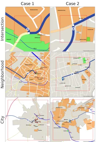
route, i.e., the start and the end of the route. For each part, we selected three prototypical locations along the route and specified the functional scales (see Figure 2). The locations were manually selected based on the authors subjective judgment in order to represent the area of an intersection, a neighborhood, and a city.
In the following, we describe the selection from OSM and apply the salience weighting. Previously, methods to assign category weights based on expert ratings (see [12]) and meth-ods to objectively retrieve category weights, e.g., from web-harvested data (see [13, 25]) were used. A sophisticated category weighting is out of scope for the current work, thus we manually assign category weights based on our subjective interpretation, taking into con-sideration previous suggestions. In addition to the category weights, the overall salience function provides parameters for weighting the different metrics. The weighting param-eters may be used to optimize the salience weighting with respect to empirical results or expert ratings. Different weights will influence the results of the salience function and they might even have to be optimized with respect to the influence of the metrics at different scales. We apply equal weights for demonstration purposes. Moreover, to demonstrate the influence of the separate metrics of the algorithm, we systematically varied the metric weights and demonstrate the results for one of the previous cases in Figure 4. In Section 5.2, we present and discuss the results of the algorithms. It is important to note, that the results might not be thecorrectselections from the conceptual perspective, however, the aim is to demonstrate the functionality of the algorithm. Future work needs to optimize the input parameters of the algorithms to generate cognitively adequate results.
5.1
Feature selection from OSM
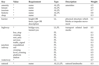
Several researchers presented methods to select landmarks from OSM by specifying OSM tag lists (e. g. [16, 48]). Although this is very selective and despite the limited availability of environmental regions in spatial databases, we use the specification in Table 4 for the can-didate selection of administrative regions (AR) and environmental regions (ER) from OSM. Environmental regions are either defined by theirboundarytag (protected_area, landuse, mar-time, national_park) or by theirlandusetag. For the former we chose the most frequent values that can be considered as ER from OSM taginfo (https://taginfo.openstreetmap.org/keys/ boundary#values); besides, theboundarytag contains many specific keys for different kinds of boundaries, e. g., political. For the latter we consider all values of thelandusetag as po-tential candidates of environmental regions. In addition, we assign category weights as shown in Table 4. After selecting region candidates and running the algorithm for calculat-ing the feature salience, the results are highlighted on a map for visual interpretation (see orange regions in Figure 3).
Key Value Requirement Type Description Weight
boundary administrative admin_level = * AR administrative boundary 1.0
boundary protected_area - ER boundary of 0.8
landuse - ER environmental region 0.3
maritime - ER 0.8
national_park - ER 0.8
landuse * - ER environmental region 1.0
Table 4: OSM tags related to structural regions
Key Value Requirement Type Description Weight
amenity * name AL,PL amenities 0.5
leisure * name AL,PL 0.5
tourism * name AL,PL 0.7
historic * name AL,PL 0.8
shop * name PL 0.3
barrier * height OR
fence_type OR description
LL physical structure which blocks or impedes move-ment
0.1
highway * bridge=yes,
tunnel=yes
LL,PL transport related land-marks
0.5
bus_stop - PL 0.1
crossing - PL 0.3
rest_area - PL 0.6
services - PL 0.4
traffic_signal - PL 0.3
junction roundabout - PL 0.6
railway rail - LL 0.7
crossing - PL 0.5
level_crossing - PL 0.5
platform - PL 0.5
station - PL 0.5
waterway * - LL 0.7
natural * name AL,LL,PL natural landmarks 0.3
Table 5: OSM tags related to landmarks
To perform the network selection (Section 4.2), the OSM data is pre-processed to gener-ate a routable graph. We use the osm2po tool (http://osm2po.de/) to pre-process the OSM data and save it to a PostgreSQL database. We implemented functions based on Postgis (https://postgis.net/) and pgRouting (https://pgrouting.org/) functionality to analyze the graph as described in Section 4.1.
5.2
Results and discussion
selected locations and target scales. The input values of the algorithm remained the same across the different runs of the algorithm. In Figure 3 the results of the algorithm are shown. Moreover, Tables 6 and 7 list the results of the single metrics as well as the final salience value. The results are dependent on the chosen data basis and the specified weights, thus might not correspond to feature selections based on empirical investigations.
In the top left and middle left map (case 1), part of the residential area is highlighted (or-ange polygon), which was selected as the most salient environmental region at that scales. However, in the bottom left map, the residential area was not selected. When closely re-viewing the separate results of the salience metrics, it turned out that the residential area got a low weight for the uniqueness metric; this is due to the OSM data structure which in this case stored the residential area as many separate small regions instead of a single large region. Similarly, we see that separate parts of the residential area were selected in the bottom right map, i.e., case 2. The respective uniqueness values are shown in Ta-ble 7. The fragmentation and granularity of OSM data depend a lot on the contributors, thus no consistency can be expected. Moreover, for the bottom left map and the middle right map, many small features were selected as environmental regions (orange polygons), which would not necessarily be defined as regions. This is due to the availability of en-vironmental regions in spatial databases, as it was discussed above; a more sophisticated description of potential region candidates would have to be specified when working with OSM data. To prioritize larger regions that would help to better structure the environment, thecoveragemetric, which is described in Section 5.2.2, might be considered for the salience function.
For linear landmarks, a river (top left, middle left, and bottom right map) and rails (middle left and bottom left map) were selected. However, in the middle and bottom map it can be seen that only part of the features were selected. This again refers to the underly-ing data structure; linear features are often divided into many features, thus the algorithm separately weights every feature. Point landmarks (red stars) and areal landmarks (green polygons) where separately selected and weighted, however, in the results the concep-tual difference between these feature types seems not clear. In OSM a landmark might be mapped as a tagged point or as a polygon when for example specifying the building footprint; quite often even both exist.
Furthermore, the direction metric was used to prioritize features in front of the current location. The resulting maps of case 1 (Figure 3 left) support the influence of this metric showing that predominantly features in front of the current location are highlighted. This is supported by the values of thedirectioncolumn in Table 6. The resulting maps of case 2 (Figure 3 right) differ especially in the bottom map. At this scales, most features lie to the back of the current location, which can also be seen in thedirectioncolumn of Table 7. While the direction metric prioritizes features to the font of the current location, the availability of the features in combination with the other metrics needs to be considered here. In the bottom right map the car is leaving the city, thus the most salient features of the city lie to the back of the current position. Consequently, the other metrics were stronger than the direction metric in this case. However, the weights of the metrics might be adjusted if required.
justed towards a lower priority of features to the front. Similarly, the relation metric, which prioritizes the relation towards a decision point, might be more relevant to be included in the overall salience function for larger scales, e.g., when identifying the salient features for the intersection scale.
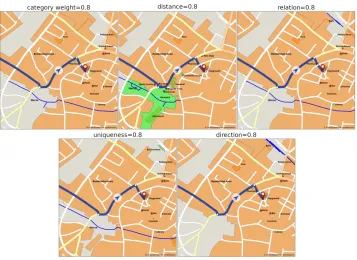
To demonstrate the influence of the separate metrics of the algorithm, we systematically varied the metric weights and demonstrate the results for one of the previous cases, i.e., case 1 neighborhood, in Figure 4. The neighborhood case was chosen, because we expected that the influence of the different metrics weights would be better visually comprehensible from the maps, compared to the intersection and city scale. Previously, equal weights for the salience metrics were applied, i.e.,ws, wr, wu, wd, wo= 0.2,Pw= 1. We systematically assign a weight of0.8to each of the metrics, whereas each of the other metrics gets a weight of0.05. We ran the algorithm once for each of the five cases; the input of the algorithm remained the same, except for the metric weight. The topmost features for each feature type were selected and visualized.
While there are overlaps in different cases, there are also differences resulting from the different weights. The biggest difference can be seen when assigning a high weight to the distance metric above the other metrics; clearly, features get selected that are closer to the current location, compared to the other cases. Slight differences appear in the results when assigning a high weight to the direction, i. e., fewer features are selected that lie to the back of the current location. Interestingly, few landmarks in the city center, i. e., Hotel, Bar, Playground, Fountain, are selected in four of five cases. This suggests, that these features have a high salience in all of the particular metrics, thus assigning a high weight to single metrics does not introduce differences. A thorough analysis of the effects of the different weights is our of scope for the current paper and should be done, if necessary,
5.2.1 General discussion
While we think that the presented algorithm can be implemented in any wayfinding sup-port system for feature selection, a few peculiarities shall be discussed here, which were revealed through the prototypical implementation and demonstration: (i) the influence of the data basis; (ii) the influence of the metrics and metric weights; (iii) the influence of the category weights.
The previous discussion of the results with respect to environmental regions and lin-ear landmarks showed, that there is an influence of thedata basison the results, namely the fragmentation of features which would subjectively be considered as a unit. When working with OSM data, a pre-processing step is required to process the data into a con-sistent data format and specifically adjust the salience weighting to the underlying data basis. Generally, the contribution of this work is an algorithm that extends previous work on the selection and salience weighting of landmarks; we especially add functionality for the context-dependence and present an adjustable and extendable method based on sep-arate salience metrics. When implementing the algorithm, the salience function has to be adapted to the selected data basis and weights have to be specified with regard to empirical evidence. Therefore, a thorough analysis of the effects of the different metric weights, as prototypically demonstrated in the previous section, might be necessary in future work.
Figure 4: Results the systematic investigation of different metric weights.
these metrics need to be chosen with respect to the use case, i. e., the feature types and the context. We specified the context with respect to the functional scales, which we proposed in a separate work [36]. Different contexts might serve different purposes, e.g., identifying an intersection or conveying orientation within a city, thus different metrics and metric weights have to be specified for the salience function with respect to the current purpose. For identifying the most salient features at a decision point, different metrics might be used than for identifying the most salient orientation information within a neighborhood or city. Finally, for getting justifiable results, empirical evidence for thecategory weightsis re-quired, which generally specifies the salience of different feature types with respect to the current purpose, not excluding human subject ratings (e.g., [43, 44]). Although previous work investigated methods for specifying category weights for landmarks (e. g. [12, 25]), the general salience of different environmental features (landmarks, network structures, structural regions) in terms of orientation support needs to be investigated in future work.
5.2.2 Extended metrics
suffice to model the overall salience of environmental features, however, additional metrics might be added to the overall salience functionSf or replace previous metrics.
Connection Related to therelation and distance metric, the connection of candidates in the candidate set might be specified, which also relates to the structural salience. The con-nection might be distinguished in terms of thedirect connection to the route, theconnection through the street network, or no connection to the route or street network. Thereby, also the distinction between local and global landmarks can be made. Moreover, candidates can be weighted differently with respect to their connection towards the route, prioritizing directly connected features. In terms of the calculation, this metric would additionally consider the adjacent street network.
Coverage When considering the visual representation, especially structural regions might be too large to be visualized on the map, e.g., large environmental regions at the neighborhood scale. Regions that cover the whole map extract will not be identifiable from the map. Therefore, acoveragemetric could be used, which weights the salience of regions in terms of the amount of overlap with the current map. On the one hand, regions that cover the whole map would be disregarded; on the other hand, the coverage would give higher weights to more overlap, assuming that more overlap is structurally more salient.
Visibility Previous research evaluated the visibility of landmarks at intersections (e.g., [42,46,59]). The work might be extended with respect to the general visibility of orientation information at decision points and along the route. While a visibility metric could easily be integrated into the previously presented salience function, we see the main challenge of this metric in the availability and processing of required data. Moreover, the visibility might not even be a static value but would be context-dependent in many aspects, e.g., time of the day, time of the year, etc.
Distribution Especially for smaller scales that aim to provide an overview of the environ-ment or an overview of the whole route, it might be necessary to consider the distribution of the selected features to avoid too much overlap and empty spots in the resulting maps. Thus, the salience of feature candidates would also depend on the location of previously selected candidates and higher weights could be assigned to features that are more distant to other features.
6
Conclusions
around decision points, but runs for any location and context along the route; (ii) beyond landmarks, our algorithm considers all kinds of orientation information. We presented a prototypical implementation of the algorithm and discussed the results.
In future work, cognitive aspects of orientation information selection need to be investi-gated. This is required for the optimization of the algorithm with respect to the underlying data basis and the theoretical input. Moreover, an open question that needs further re-search, is the representation and selection of environmental regions in spatial databases. While previous work focused on static scenarios, we see the biggest challenge in the selec-tion and visualizaselec-tion of cognitive adequate orientaselec-tion informaselec-tion for dynamic wayfind-ing scenarios. Future work needs to investigate how the salience and relevance of envi-ronmental features for wayfinding and orientation support changes with respect to the changing context of the navigators. Moreover, algorithms need to be extended to account for context changes along the route.
Acknowledgments
This project has received funding from the European Research Council (ERC) under the European Union’s Horizon 2020 research and innovation programme (grant agreement n◦ 637645).
References
[1] ANACTA, V. J. A., HUMAYUN, M. I., SCHWERING, A.,ANDKRUKAR, J. Investigating Representations of Places with Unclear Spatial Extent in Sketch Maps. InSocietal Geo-innovation: Selected papers of the 20th AGILE conference on Geographic Information Science, A. Bregt, T. Sarjakoski, R. van Lammeren, and F. Rip, Eds. Springer, Cham, 2017, pp. 3– 17. doi:10.1007/978-3-319-56759-4_1.
[2] ANACTA, V. J. A., LI, R., LÖWEN, H., DE LIMA GALVAO, M., AND SCHWERING, A. Spatial Distribution of Local Landmarks in Route-Based Sketch Maps. InSpatial Cognition XI, S. H. Creem-Regehr, J. Schöning, and A. Klippel, Eds. Springer, Cham, Switzerland, 2018, pp. 107–118. doi:10.1007/978-3-319-96385-3_8.
[3] ANACTA, V. J. A., SCHWERING, A., LI, R., ANDMÜNZER, S. Orientation informa-tion in wayfinding instrucinforma-tions: evidences from human verbal and visual instrucinforma-tions. GeoJournal 82, 3 (6 2017), 567–583. doi:10.1007/s10708-016-9703-5.
[4] BRÜGGER, A., RICHTER, K.-F.,ANDFABRIKANT, S. I. How does navigation system behavior influence human behavior? Cognitive Research: Principles and Implications 4, 1 (2019), 5. doi:10.1186/s41235-019-0156-5.
[5] BURNETT, G. E., ANDLEE, K. The Effect of Vehicle Navigation Systems on the For-mation of Cognitive Maps. InInternational Conference of Traffic and Transport Psychology (Amsterdam, The Netherlands, 2005), G. Underwood, Ed., Elsevier.
[7] CLARAMUNT, C., AND WINTER, S. Structural Salience of Elements of the City. Environment and Planning B: Planning and Design 34, 6 (2007), 1030–1050. doi:10.1068/b32099.
[8] DANIEL, M.-P., AND DENIS, M. Spatial Descriptions as Navigational Aids: A Cognitive Analysis of Route Directions. Kognitionswissenschaft 7, 1 (2 1998), 45–52. doi:10.1007/BF03354963.
[9] DENIS, M. The description of routes: A cognitive approach to the production of spatial discourse.Cahiers de psychologie cognitive 16, 4 (1997), 409–458.
[10] DIJKSTRA, E. W. A note on two problems in connexion with graphs. Numerische mathematik 1, 1 (1959), 269–271. doi:10.1007/BF01386390.
[11] DUCKHAM, M., AND KULIK, L. “Simplest” Paths: Automated Route Selection for Navigation. InSpatial Information Theory. Foundations of Geographic Information Sci-ence: International Conference, COSIT 2003, Kartause Ittingen, Switzerland, September 24-28, 2003. Proceedings, W. Kuhn, M. F. Worboys, and S. Timpf, Eds. Springer, Berlin, Heidelberg, 2003, pp. 169–185. doi:10.1007/978-3-540-39923-0_12.
[12] DUCKHAM, M., WINTER, S., AND ROBINSON, M. Including landmarks in routing instructions. Journal of Location Based Services 4, 1 (3 2010), 28–52. doi:10.1080/17489721003785602.
[13] ELIAS, B. Extracting Landmarks with Data Mining Methods. InSpatial Information Theory. Foundations of Geographic Information Science: International Conference, COSIT 2003(Berlin, Heidelberg, 2003), W. Kuhn, M. F. Worboys, and S. Timpf, Eds., Springer, pp. 375–389. doi:10.1007/978-3-540-39923-0_25.
[14] FISHER, D. H. Knowledge acquisition via incremental conceptual clustering.Machine Learning 2, 2 (9 1987), 139–172. doi:10.1007/BF00114265.
[15] GALTON, A. On the Ontological Status of Geographic Boundaries. Foundations of Geographic Information Science(2003), 160–182.
[16] GRASER, A. Towards landmark-based instructions for pedestrian navigation systems using OpenStreetMap. InSocietal Geo-Innovation : short papers, posters and poster ab-stracts of the 20th AGILE Conference on Geographic Information Science. Wageningen Uni-versity & Research 9-12 May 2017(Wageningen, The Netherlands, 2017), A. Bregt, T. Sar-jakoski, R. v. Lammeren, and F. Rip, Eds.
[17] HANSEN, S., RICHTER, K.-F., AND KLIPPEL, A. Landmarks in OpenLS - A Data Structure for Cognitive Ergonomic Route Directions. InGeographic Information Sci-ence: 4th International Conference, GIScience 2006, M. Raubal, H. J. Miller, A. U. Frank, and M. F. Goodchild, Eds. Springer, Münster, Germany, 2006, pp. 128–144. doi:10.1007/11863939_9.
[19] HILLIER, B., ANDHANSON, J. The social logic of space. Cambridge University Press, Cambridge, 1984.
[20] HUMAYUN, M. I.,ANDSCHWERING, A. Selecting a Representation for Spatial Vague-ness: A Decision Making Approach. InGeographic Information Science at the Heart of Europe, D. Vandenbroucke, B. Bucher, and J. Crompvoets, Eds. Springer, 2013, pp. 115– 131. doi:10.1007/978-3-319-00615-4_7.
[21] ISHIKAWA, T., FUJIWARA, H., IMAI, O., AND OKABE, A. Wayfinding with a GPS-based mobile navigation system: A comparison with maps and direct experience. Journal of Environmental Psychology 28, 1 (2008), 74–82. doi:10.1016/j.jenvp.2007.09.002.
[22] JIANG, B., AND LIU, X. Computing the fewest-turn map directions based on the connectivity of natural roads. International Journal of Geographical Information Science 25, 7 (2011), 1069–1082. doi:10.1080/13658816.2010.510799.
[23] JIANG, B., ZHAO, S.,ANDYIN, J. Self-organized natural roads for predicting traffic flow: a sensitivity study.Journal of Statistical Mechanics: Theory and Experiment 2008, 07 (2008), P07008. doi:10.1088/1742-5468/2008/07/p07008.
[24] KATTENBECK, M., NUHN, E., AND TIMPF, S. Is Salience Robust? A Het-erogeneity Analysis of Survey Ratings. In 10th International Conference on Geo-graphic Information Science (GIScience 2018) (Dagstuhl, Germany, 2018), S. Winter, A. Griffin, and M. Sester, Eds., vol. 114 of Leibniz International Proceedings in In-formatics (LIPIcs), Schloss Dagstuhl–Leibniz-Zentrum fuer Informatik, pp. 7:1–7:16. doi:10.4230/LIPIcs.GISCIENCE.2018.7.
[25] KIM, J., VASARDANI, M., AND WINTER, S. Landmark Extraction from Web-Harvested Place Descriptions. KI - Künstliche Intelligenz 31, 2 (5 2017), 151–159. doi:10.1007/s13218-016-0467-3.
[26] KLIPPEL, A., HANSEN, S., RICHTER, K.-F.,ANDWINTER, S. Urban granularities - A data structure for cognitively ergonomic route directions. GeoInformatica 13, 2 (2009), 223–247. doi:10.1007/s10707-008-0051-6.
[27] KLIPPEL, A., AND MONTELLO, D. R. Linguistic and Nonlinguistic Turn Direction Concepts. InSpatial Information Theory: 8th International Conference, COSIT 2007, Mel-bourne, Australiia, S. Winter, M. Duckham, L. Kulik, and B. Kuipers, Eds. Springer, Berlin, Heidelberg, 2007, pp. 354–372. doi:10.1007/978-3-540-74788-8_22.
[28] KLIPPEL, A., TAPPE, H.,ANDHABEL, C. Pictorial Representations of Routes: Chunk-ing Route Segments durChunk-ing Comprehension. InSpatial Cognition III: Routes and Naviga-tion, Human Memory and Learning, Spatial Representation and Spatial Learning, C. Freksa, W. Brauer, C. Habel, and K. F. Wender, Eds. Springer, Berlin, Heidelberg, 2003, pp. 11– 33. doi:10.1007/3-540-45004-1_2.
[30] KLIPPEL, A., AND WINTER, S. Structural Salience of Landmarks for Route Direc-tions. InSpatial Information Theory: International Conference, COSIT 2005, Ellicottville, NY, USA, September 14-18, 2005. Proceedings, A. G. Cohn and D. M. Mark, Eds. Springer, Berlin, Heidelberg, 2005, pp. 347–362. doi:10.1007/11556114_22.
[31] KRÜGER, A., ASLAN, I., AND ZIMMER, H. The Effects of Mobile Pedestrian Navi-gation Systems on the Concurrent Acquisition of Route and Survey Knowledge. In Mobile Human-Computer Interaction - MobileHCI 2004, S. Brewster and M. Dunlop, Eds. Springer Berlin Heidelberg, Berlin, Heidelberg, 2004, pp. 446–450. doi:10.1007/978-3-540-28637-0_54.
[32] KRUKAR, J., AND SCHWERING, A. What is Orientation? InProceedings of the 13th Biannual Conference of the German Cognitive Science Society(Bremen, Germany, 2016), T. Barkowsky, Z. F. Llansola, H. Schultheis, and J. van de Ven, Eds., KogWis: Space for Cognition, pp. 115–118.
[33] LI, R., KORDA, A., RADTKE, M.,ANDSCHWERING, A. Visualising distant off-screen landmarks on mobile devices to support spatial orientation. Journal of Location Based Services 8, 3 (2014), 166–178. doi:10.1080/17489725.2014.978825.
[34] LOVELACE, K. L., HEGARTY, M.,ANDMONTELLO, D. R. Elements of Good Route Directions in Familiar and Unfamiliar Environments. InSpatial Information Theory. Cognitive and Computational Foundations of Geographic Information Science, C. Freksa and D. M. Mark, Eds. Springer, Berlin, Heidelberg, 1999, pp. 65–82. doi:10.1007/3-540-48384-5_5.
[35] LÖWEN, H., KRUKAR, J.,ANDSCHWERING, A. How should Orientation Maps look like? InGeospatial Technologies for All: short papers, posters and poster abstracts of the 21th AGILE Conference on Geographic Information Science. Lund University 12-15 June 2018, Lund, Sweden(Cham, Switzerland, 2018), A. Mansourian, P. Pilesjö, L. Harrie, and R. van Lammeren, Eds., Springer.
[36] LÖWEN, H., KRUKAR, J., AND SCHWERING, A. Functional Scales in Assisted Wayfinding. InProceedings of the 14th International Conference on Spatial Information Theory (COSIT 2019) (Dagstuhl, Germany, 2019), S. Timpf, C. Schlieder, M. Katten-beck, B. Ludwig, and K. Stewart, Eds., vol. 142 ofLeibniz International Proceedings in Informatics (LIPIcs), Schloss Dagstuhl–Leibniz-Zentrum fuer Informatik, pp. 3:1–3:7. doi:10.4230/LIPIcs.COSIT.2019.3.
[37] LÖWEN, H., KRUKAR, J., AND SCHWERING, A. Spatial Learning with Orienta-tion Maps: The Influence of Different Environmental Features on Spatial Knowl-edge Acquisition. ISPRS International Journal of Geo-Information 8, 3 (3 2019). doi:10.3390/ijgi8030149.
[39] MICHON, P.-E., AND DENIS, M. When and Why Are Visual Landmarks Used in Giving Directions? InSpatial Information Theory: Foundations of Geographic Informa-tion Science InternaInforma-tional Conference, COSIT 2001 Morro Bay, CA, USA, September 19–23, 2001 Proceedings, D. R. Montello, Ed. Springer, Berlin, Heidelberg, 2001, pp. 292–305. doi:10.1007/3-540-45424-1_20.
[40] MÜNZER, S., LÖRCH, L.,ANDFRANKENSTEIN, J. Wayfinding and acquisition of spa-tial knowledge with navigation assistance. Journal of experimental psychology. Applied (2019). doi:10.1037/xap0000237.
[41] MÜNZER, S., ZIMMER, H. D., AND BAUS, J. Navigation assistance: A trade-off be-tween wayfinding support and configural learning support. Journal of Experimental Psychology: Applied 18, 1 (2012), 18–37. doi:10.1037/a0026553.
[42] NOTHEGGER, C., WINTER, S., AND RAUBAL, M. Selection of Salient Features for Route Directions. Spatial Cognition & Computation 4, 2 (6 2004), 113–136. doi:10.1207/s15427633scc0402_1.
[43] NUHN, E., AND TIMPF, S. A multidimensional model for selecting person-alised landmarks. Journal of Location Based Services 11, 3-4 (2017), 153–180. doi:10.1080/17489725.2017.1401129.
[44] QUESNOT, T., AND ROCHE, S. Measure of Landmark Semantic Salience through Geosocial Data Streams.ISPRS International Journal of Geo-Information 4, 1 (2015), 1–31. doi:10.3390/ijgi4010001.
[45] QUINLAN, J. R. Induction of decision trees. Machine Learning 1, 1 (1986), 81–106. doi:10.1007/BF00116251.
[46] RAUBAL, M., ANDWINTER, S. Enriching Wayfinding Instructions with Local Land-marks. InGeographic Information Science: Second International Conference, GIScience 2002 (Boulder, CO, USA, 2002), M. J. Egenhofer and D. M. Mark, Eds., Lecture Notes in Computer Science, Springer, pp. 243–259. doi:10.1007/3-540-45799-2_17.
[47] RICHTER, K.-F.,ANDWINTER, S.Landmarks: GIScience for Intelligent Services. Springer, Cham, Switzerland, 2014.
[48] ROUSELL, A., ANDZIPF, A. Towards a Landmark-Based Pedestrian Navigation Ser-vice Using OSM Data. ISPRS International Journal of Geo-Information 6, 3 (2 2017), 64. doi:10.3390/ijgi6030064.
[49] SCHMID, F. Knowledge-based wayfinding maps for small display cartography.Journal of Location Based Services 2, 1 (3 2008), 57–83. doi:10.1080/17489720802279544.
[50] SCHOCKAERT, S., SMART, P. D.,AND TWAROCH, F. A. Generating approximate re-gion boundaries from heterogeneous spatial information: An evolutionary approach. Information Sciences 181, 2 (2011), 257–283. doi:10.1016/j.ins.2010.09.021.
[52] SESTER, M.,ANDDALYOT, S. Enriching Navigation Instructions to Support the For-mation of Mental Maps. InAdvances in Spatial Data Handling and Analysis: Select Pa-pers from the 16th IGU Spatial Data Handling Symposium, F. Harvey and Y. Leung, Eds. Springer, 2015, pp. 15–33. doi:10.1007/978-3-319-19950-4_2.
[53] SMITH, B., AND MARK, D. M. Ontology and Geographic Kinds. Proceedings. 8th International Symposium on Spatial Data Handling (SDHâ ˘A ´Z98)(1998), 267–282.
[54] SORROWS, M. E., AND HIRTLE, S. C. The Nature of Landmarks for Real and Elec-tronic Spaces. InSpatial Information Theory. Cognitive and Computational Foundations of Geographic Information Science: International Conference COSIT’99 Stade, Germany, Au-gust 25–29, 1999 Proceedings, C. Freksa and D. M. Mark, Eds. Springer, Berlin, Heidel-berg, 1999, pp. 37–50. doi:10.1007/3-540-48384-5_3.
[55] STECK, S. D.,ANDMALLOT, H. A. The Role of Global and Local Landmarks in Virtual Environment Navigation.Presence: Teleoperators and Virtual Environments 9, 1 (2 2000), 69–83. doi:10.1162/105474600566628.
[56] TOM, A., AND DENIS, M. Referring to Landmark or Street Information in Route Directions: What Difference Does It Make? In Spatial Information Theory. Founda-tions of Geographic Information Science: International Conference, COSIT 2003, W. Kuhn, M. F. Worboys, and S. Timpf, Eds. Springer, Berlin, Heidelberg, 2003, pp. 362–374. doi:10.1007/978-3-540-39923-0_24.
[57] TOMKO, M., AND WINTER, S. Pragmatic Construction of Destination Descrip-tions for Urban Environments. Spatial Cognition & Computation 9, 1 (2009), 1–29. doi:10.1080/13875860802427775.
[58] TOMKO, M., AND WINTER, S. Describing the functional spatial structure of ur-ban environments. Computers, Environment and Urban Systems 41 (2013), 177–187. doi:10.1016/j.compenvurbsys.2013.05.002.
[59] WINTER, S. Route Adaptive Selection of Salient Features. InSpatial Information The-ory. Foundations of Geographic Information Science: International Conference, COSIT 2003, Kartause Ittingen, Switzerland, September 24-28, 2003. Proceedings, W. Kuhn, M. F. Wor-boys, and S. Timpf, Eds. Springer, Kartause Ittingen, Switzerland, 2003, pp. 349–361. doi:10.1007/978-3-540-39923-0_23.
[60] WINTER, S., TOMKO, M., ELIAS, B., AND SESTER, M. Landmark Hierarchies in Context. Environment and Planning B: Planning and Design 35, 3 (6 2008), 381–398. doi:10.1068/b33106.
Feature Category
Type Name Weight Relation Uniqueness Distance Direction Salience
Intersection
PL Wayside Cross 0.80 1.00 1.00 0.80 1.00 0.92
PL Memorial 0.80 1.00 1.00 0.64 1.00 0.89
LL Werse 0.70 1.00 1.00 0.21 0.50 0.68
AL Westpark 0.50 1.00 1.00 0.97 1.00 0.89
ER Residential Area 1.00 1.00 1.00 1.00 1.00 1.00
Neighborhood
PL Hotel 0.70 1.00 1.00 0.80 1.00 0.90
PL Bar 0.50 1.00 1.00 0.72 1.00 0.84
PL Dentist 0.50 1.00 1.00 0.61 1.00 0.82
PL Bank 0.50 1.00 1.00 0.57 1.00 0.81
PL Driving School 0.50 1.00 1.00 0.50 1.00 0.80
LL Rails 0.70 1.00 0.14 0.29 1.00 0.63
LL Rails 0.70 1.00 0.14 0.28 1.00 0.63
LL Rails 0.70 1.00 0.14 0.27 1.00 0.62
LL Werse 0.70 1.00 0.20 0.61 0.50 0.60
LL Werse 0.70 1.00 0.20 0.84 0.10 0.57
AL Playground 0.50 1.00 1.00 0.96 1.00 0.89
AL Fountain 0.50 1.00 1.00 0.64 1.00 0.83
AL Pharmacy 0.50 1.00 0.50 0.98 1.00 0.80
AL Library 0.50 1.00 1.00 0.43 1.00 0.79
AL Hotel 0.70 1.00 1.00 0.71 0.50 0.78
ER Residential Area 1.00 1.00 0.50 1.00 1.00 0.90
City
PL Hotel 0.70 1.00 1.00 0.95 1.00 0.93
PL Bar 0.50 1.00 1.00 0.92 1.00 0.88
PL Casino 0.50 1.00 1.00 0.86 1.00 0.87
PL Radio Station 0.50 1.00 1.00 0.81 1.00 0.86
PL Main Train Station 0.50 1.00 1.00 0.78 1.00 0.86
LL Rails 0.70 1.00 0.03 0.80 1.00 0.71
LL Rails 0.70 1.00 0.03 0.80 1.00 0.71
LL Rails 0.70 1.00 0.03 0.80 1.00 0.71
LL Rails 0.70 1.00 0.03 0.78 1.00 0.70
LL Rails 0.70 1.00 0.03 0.78 1.00 0.70
AL City Council 0.80 1.00 1.00 0.98 1.00 0.96
AL Hotel 0.70 1.00 1.00 0.92 1.00 0.92
AL Swimming Pool 0.70 1.00 1.00 0.76 1.00 0.89
AL Library 0.50 1.00 1.00 0.84 1.00 0.87
AL Hospital 0.50 1.00 1.00 0.80 1.00 0.86
ER Railway 1.00 1.00 1.00 0.80 1.00 0.96
ER Construction Site 1.00 1.00 1.00 0.76 1.00 0.95
ER Cementery 1.00 1.00 0.50 0.64 1.00 0.83
ER Allotments 1.00 1.00 0.14 0.91 1.00 0.81
ER Allotments 1.00 1.00 0.14 0.78 1.00 0.79
Feature Category
Type Name Weight Relation Uniqueness Distance Direction Salience
Intersection
PL Bus Stop 0.10 1.00 1.00 0.92 1.00 0.80
AL Sports Center 0.50 1.00 1.00 0.83 0.10 0.69
ER Commercial 1.00 1.00 1.00 0.63 0.50 0.83
ER Residential Area 1.00 0.50 0.33 0.91 1.00 0.75
Neighborhood
PL Sports Club 0.50 1.00 1.00 0.78 0.10 0.68
PL Internet Cafe 0.50 1.00 1.00 0.63 0.10 0.65
PL Bus Stop 0.10 1.00 0.06 0.99 1.00 0.63
PL Bus Stop 0.10 1.00 0.06 0.99 1.00 0.63
PL Bank 0.50 0.50 0.50 0.60 1.00 0.62
AL School 0.50 1.00 0.50 0.78 1.00 0.76
AL McDonalds 0.50 1.00 1.00 0.45 0.50 0.69
AL Kindergarden 0.50 1.00 0.33 0.42 1.00 0.65
AL Playground 0.50 0.50 0.33 0.90 1.00 0.65
AL Restaurant 0.50 1.00 1.00 0.20 0.50 0.64
ER Garages 1.00 1.00 0.05 0.98 1.00 0.81
ER Park 1.00 0.50 0.50 0.98 1.00 0.80
ER Trees 1.00 1.00 1.00 0.45 0.50 0.79
ER Garages 1.00 1.00 0.05 0.85 1.00 0.78
ER Allotments 1.00 0.50 0.50 0.80 1.00 0.76
City
PL Community Center 0.50 1.00 1.00 0.85 0.10 0.69
PL Mosque 0.50 1.00 1.00 0.74 0.10 0.67
PL City Hotel 0.70 1.00 1.00 0.47 0.10 0.65
LL Olfe 0.70 0.50 0.50 0.93 1.00 0.73
LL Werse 0.70 1.00 0.33 0.63 0.10 0.55
LL Werse 0.70 1.00 0.33 0.49 0.10 0.52
LL Werse 0.70 1.00 0.33 0.47 0.10 0.52
AL Retirement Home 0.50 1.00 1.00 0.74 0.10 0.67
AL Police 0.50 1.00 1.00 0.62 0.10 0.64
AL Stadium 0.50 1.00 1.00 0.59 0.10 0.64
AL Court 0.50 1.00 1.00 0.52 0.10 0.62
AL Swimming Pool 0.50 1.00 1.00 0.46 0.10 0.61
ER Industrial Area 1.00 0.50 0.50 1.00 1.00 0.80
ER Farmland 1.00 0.50 0.05 0.95 1.00 0.70
ER Residential Area 1.00 0.50 0.04 1.00 0.50 0.61
ER Residential Area 1.00 0.50 0.04 0.64 0.50 0.54
ER Residential Area 1.00 0.50 0.04 0.46 0.10 0.42
![Table 1: Functional scales in wayfinding support (reproduced from Löwen et al. [36]).](https://thumb-us.123doks.com/thumbv2/123dok_us/1157798.1617892/5.612.117.511.368.580/table-functional-scales-waynding-support-reproduced-lowen-et.webp)