RESEARCH ARTICLE
VOLUME EQUALIZATION METHOD FOR LAND GRADING DESIGN: UNIFORM SLOPED GRADING IN
TWO DIRECTIONS AT RECTANGULAR FIELDS
1
Kadir E. TEMIZEL and
2, *Yasar AYRANCI
1
Ondokuz Mayis University, Agricultural Faculty, Department of Agricultural Structures and Irrigation,
55139 Kurupelit, Samsun, TURKEY
2
Mugla Sitki Kocman University, Kazim Yilmaz Polytechnic, Aatca, Mugla, TURKEY
ARTICLE INFO
ABSTRACT
This paper presents a new method (Volume Equalization Method-VEM) which has been developed to perform land grading design at designing the uniform sloped grading in two directions. The method is a second design alternative of the method developed by Ayranci and Temizel (2011) which about uniform sloped grading in one direction at rectangular fields. The main goal of this method is to minimize the volumes of earth work required for acceptable smooth surface. The method based on the assumption that before and after grading the soil volumes measured from a reference elevation are equal. The method eliminates the need for trial and error procedures. According to the results of the application for a known slope values in X and Y directions for a hypothetical area about 2.21 ha, the cut volumes per hectare for Least Square Method and Volume Equalization Method are 419.5 m3 and 403.2 m3 respectively. According to the results, it can be expressed that Volume Equalization Method has a significantly smaller cut volume than conventional least-squares method in rectangular fields.
Copyright © 2016,Kadir E. TEMIZEL and Yasar AYRANCI.This is an open access article distributed under the Creative Commons Attribution License, which permits unrestricted use, distribution, and reproduction in any medium, provided the original work is properly cited.
INTRODUCTION
Land grading (or leveling, or smoothing) is the process of moving soil from high spots on the land surface to low spots to provide a more uniform plane for water flow. Land grading usually improves the uniformity of water application within basins, borders, and furrows (L.G. James, 1988). Land leveling always improves the efficiency of water, labor and energy resources utilization. The leveling operation, however, can be the most intensively disruptive cultural practice applied to the field and several factors should be considered before implementing a land leveling project (W.R. Walker, 1989). Land grading designs were first accomplished by elementary calculations using trial-and-error (S.N. Hamad and A.M. Ali, 1990). The first systematic procedure to perform land-grading designs for rectangular plots is used by Givan (1940). The method was based on least-squares theory. G.E. Chugg (1947) also used least-squares method (LSM) but, in irregularly shaped plots. The Average Profile Method (APM) developed by J.C. Marr (1957) is also based on the LSM theory and can be used in rectangular fields. W.S. Harris et al, (1966) introduced a new method to define a best-fit warped surface.
*Corresponding author: Yasar AYRANCI,
Mugla Sitki Kocman University, Kazim Yilmaz Polytechnic, Aatca, Mugla, TURKEY.
Such a surface has variable slope in the irrigation direction, while the cross-irrigation slope follows the natural ground
profile with minor modifications. N.A. Gebre-Selassie and
L.S. Willardson (1991) introduced a user-friendly land-leveling program developed for the computation scheme presented by E.J. Scallopi and L.S. Willardson (1986). S.P. Shih and G.J. Kriz (1971) introduced the symmetrical residuals method (SRM) to grade lands that allows for uniform or non-uniform slopes in both directions. The method can be used for five design alternatives: (a) uniform slopes allowing drainage in both directions, (b) variable slopes allowing drainage in both directions, (c) uniform slope along the individual profiles in one direction and variable slope in the other and allowing drainage in both directions, (d) uniform slope along individual profiles allowing drainage in one direction and minimum and maximum allowable slopes in the other direction, and (e) variable slope along individual profiles allowing drainage in one direction and minimum and maximum allowable slopes in the other direction. S.N. Hamad and A.M. Ali (1990) used a new technique using non-linear programming to fit a curved or a plane-graded surface to the natural ground surface. L.R. Srinivasa (1996) developed a nonlinear optimization model based on genetic algorithms for land grading design of irregular fields. Another method proposed by (Easa 1998) explicitly considers the required design specifications which may include the two edge slopes
ISSN: 0976-3376
Vol. 07, Issue, 10, pp.3620-3626, October,Asian Journal of Science and Technology 2016Available Online at http://www.journalajst.com
ASIAN JOURNAL OF
SCIENCE AND TECHNOLOGY
Article History:
Received 15th July, 2016 Received in revised form 20th August, 2016
Accepted 24th September, 2016
Published online 30th October, 2016
Key words:
of the plane, one edge slope and a control point, or two control
points. A land-leveling system provided by (K.R.
Zimmermann et al, 2005) which use the Global Positioning System (GPS). Lately, Y. Ayranci and K.E. Temizel (2011) presented a new method (Volume Equalization Method-VEM) to perform land grading design in designing the uniform sloped grading in one direction in rectangular fields. This research presents a new method (VEM) which a second design alternative of the method developed by Y. Ayranci and K.E. Temizel (2011) to design a uniform sloped grading in two directions at rectangular (or square) fields. The method uses the principle which also used by V.S. Raju (1960) and by S.M. Easa (1998) that the volume under the original ground surface is equal to the volume under the computed land grading plane.
MATERIAL AND METHODS
Land grading is performed on land where surface irrigation techniques are employed, in order to increase the efficiency of irrigation. Therefore, land was rendered compatible with the slope values required by the irrigation method via land grading. Depending on the irrigation method to be employed, land can be graded according to one of grading types such as uniformed sloped grading in one direction, uniform sloped grading in two directions, variable sloped grading in one direction and variable sloped grading in two directions or in accordance with the natural slope of the land. In this study, the application of uniform sloped grading in two directions of VEM on smooth patterned lands was issued.
Uniform Sloped Grading in Two Directions
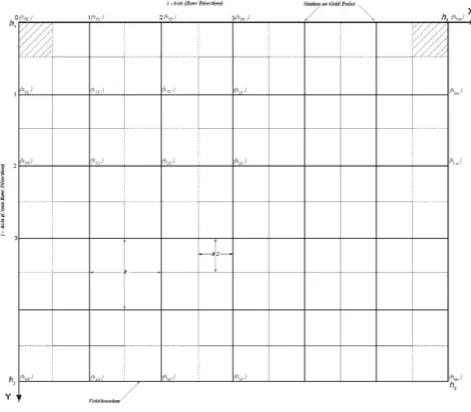
A field layout and the adopted coordinate system are shown in
Figure 1. The grid elevations, hij (i=1,2,3…,nj in row direction
and j=1,2,3…,mi in cross row direction) were taken at equal
intervals, d. The numbers of rows and cross rows may not be equal. In this case, the stations (grid points) are forming an
mxn sized matrix. There was distance of half a square length
between a grid point and land borders. Thus, each station-grid point represented square shaped land with a side length of d. However, the area represented by each grid point was not always square shaped. Sometimes this area may be bigger or smaller than one unit of square. The area represented by any
station (Fij), was the area formed by connecting the side
midpoints of the station and adjacent stations (Figure 1). For
instance, grid points such as h11, h21, h23, h32 represented the
areas of 1.0 unit, h1m, h2m, h3m grid points represented areas
bigger than 1.0 unit and grid point like hn1, hn2, hnm represented
areas smaller than 1.0 unit. The grid elevation of each grid point determined was measured and transferred to a CAD program. The grid elevations in every row and cross row were
summed up to obtain ∑Hi and ∑Hj values and their means
were calculated to acquire Hi mean and Hj mean values (Figure 1).
Hi mean ve Hj mean values could be found with the help of the
equations (Y. Ayranci and K.E. Temizel 2011) below.
Hi mean=
∑ ∗
(1)
Hj mean=
∑ ∗
(2)
where Hi mean is the value of the mean of ith row (m), Hj mean is
the value of the mean of jth cross row (m), hij is the grid
elevation of ith row at jth cross row (m), Fij is the unit area of
grid of a ith row at jth cross row (m2), m is the number of unit
grids at the j direction, and n is the number of unit grids at the i direction.
Figure 1. Field layout and the adopted coordinates system
In the CAD program, contours were drawn with required intervals as coordinates and elevation values were entered for each grid and land borders were taken into consideration. Then, areas between every contour (i.e., the area between the contours 2.3 m and 2.4 m in Figure 1) within the land borders were calculated one by one with the help of the program. The sum of the areas between contour lines and the areas out of the contour lines equal to the projection area (F) of the land will be graded.
Volume Before Grading
The significance of the method lies in the calculation of the amount of the soil in the land which is to be graded based on a reference plane and utilization of this soil volume in grading process. The equation below (Ayranci and Temizel 2011) is used to calculate the volume of soil between two consecutive grading curves.
= ∗ (3)
where Vz is the volume of soil between two consecutive
grading curves (m3), cz is the elevation of the smaller one of
the grading curves of which the volume of soil was calculated,
(m), cz+1 is the elevation of the bigger one of the grading
curves of which the volume of soil was calculated (m), and Fz
is the projection area between the two grading curve of which
the volume of soil to be calculated (m2). On every land, there
were land fractions higher than the biggest grading curve and lower than the smallest grading curve. The calculation of soil
volume (Vad) in these fields, the elevation values of the grading
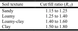
curves and the border point of the land in that field can be used with the help of equation 3. For example, on the calculation of the soil volume of the grey colored area in figure 2(A); 3.0 m
contour line can be taken as cz value and the average of the
points 3.02, 3.03 and 3.05 m can be taken as cz+1 value (3.033).
The total soil volume before grading (Vbg) can be obtained by
Hence, the total soil volume before grading can be found with the help of equation 4 (Y. Ayranci and K.E. Temizel 2011).
= ∑ + (4)
where Vbg is the total soil volume before grading (m3), Vad is
soil volume belonging to the field outside of grading curves
(m3), z is the number of areas between grading curves
(z=1,2,3,…..,z), and Vz is the soil volume between the two
grading curves consecutive (m3).
Volume After Grading
According to the principle of “soil should not be brought from
another place to the land which is to be graded, nor should it be removed from the land which is to be graded to another place” which is among the basic rules of land grading, the soil
volume before grading (Vbg) should be equal (Vbg=Vag) to the
soil volume after grading (Vag). This form of grading is
especially preferred by the Furrow Irrigation method. Because of after application of uniform slope grading in two directions all the heights of land corners will be different the total soil volume after grading can be calculated by the following equation 5.
= ∗ (5)
where Vag is the total soil volume after grading (m3), h1, h2, h3
and h4 are after grading heights of the corners of the land (m),
and F is the projection area of the land to be graded (m2). At
this stage it should be decided in which direction the land should be graded and how much slope should be given; a decision between the directions X and Y and the amounts of slope. This decision is affected by the following two possibilities:
The irrigation method (or the land owner's request, etc.)
is an important factor for the decision of direction and slope of the land grading.
Another possibility is to grade the land according to its
natural slope.
If Slope Values in X and Y Directions Are Predetermined
Uniform sloped grading in two directions with known slope (requested or provided) in X and Y directions can be explained as follows. After application of uniform sloped grading in two directions, the elevation values of all corners of the land will be different.
h1≠h2≠h3≠h4 (6)
Accordingly, after grading the elevation values of land corners 2, 3 and 4 can be calculated by means of the following equations 7, 8, and 9.
ℎ = ℎ ∓ ∗ (7)
ℎ = ℎ ∓ ∗ (8)
ℎ = ℎ ∓ ∗ (9)
where Mx is the requested/provided slope value in X direction
(%), My is the requested/provided slope value in Y direction
(%), Lx is the length of the land in X direction (m). Ly is the
length of the land in Y direction, m. If equations 7 and 9 are put in equation 5, equation 5 will be as follows.
= ∓
∗
∗ (10)
If equation 8 is put in equation 10 and the necessary simplifications are made, equation 10 will be as follows.
= ∓
∗
∓ ∗
∗ (11)
Following equation 12 which can be used in finding the
elevation of the corner point h1, can be obtained from equation
11.
ℎ = ∓
∗
∓ ∗
(12)
After the determination of corner point (h1), the elevations of
the corner point’s h2, h3 and h4 determined by equations 7, 8
and 9 respectively. The height of the grid point h1,1 can be
found with the help of equation 14.
ℎ , = ℎ ∓
∗
∓ ∗ (13)
where h1,1 is the height of the grid point 1,1 (m), Ls is the side
length of grid (m). After finding the height of grid point 1,1 after grading, the heights of following points in X and Y directions can also be found by helping equation 14 and 15.
ℎ , = ℎ , ∓
∗
(14)
ℎ , = ℎ , ∓
∗
(15)
The heights of the following grid points in X and Y directions are found in the same way. In this way, the heights of all grid points of the land are found. The heights in the grids, found by calculation are compared with the natural heights in the grids. The heights of cut and fill for every grid points are determined accordingly. According to the found cut and fill heights, the cut and fill volumes are determined for each grid. By calculating of the volume of cut and fill on any grid, the values of cut or fill in that grid in m is multiplied by the value of the
area unit in m2 of the grid (equations 16 and 17 [Y. Ayranci
and K.E. Temizel 2011]). If the slope values of X and Y directions is positive (sign +), if negative (sign –) are used in equations 7, 8, 9, 10, 11, 12, 13, 14, and 15.
= ℎ ∗ (16)
= ℎ ∗ (17)
where Vpc is the volume of cut at the pth grid (m3), hpc is the
height of cut at the pth grid (m), Fpc is the unit area of pth grid
(m2), Vrf is the volume of fill at p
th
grid (m3), hrf is the height of
The total volume of cut and fill equals the sum of cut and fill volumes (equations 18 and 19 [Y. Ayranci and K.E. Temizel 2011]) of each grid.
= ∑ (18)
= ∑ (19)
where Vc is the total cut volume (m
3
), Vf is the total fill volume
(m3), p is the number of cut grid (p=1,2,3,…..,p), and r is the
number of fill grid (r=1,2,3,….,r).
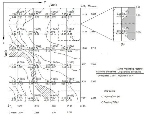
The cut/fill ratio (Rc/f) is found by dividing the total cut volume into the total fill volume. In land grading, according to the soil texture, cut/fill ratio is requested to be in the ranges of the values given in table 1. If the cut/fill ratio is within the desired limits, the grading operation is performed according to its specified values.
Table 1. Cut/fill ratio limits according to the soil texture (Rc/f)
Soil texture Cut/fill ratio (Rc/f)
Sandy Loamy Loamy-clay Clay
1.15 to 1.25 1.25 to 1.40 1.40 to 1.60 1.50 to 1.80
If the cut/fill ratio found is not within the limits, the grading plane height should be changed. In this case, the amount of the change to be done on the height of the grading plane can be found with the help of the equation 20 (Y. Ayranci and K.E. Temizel 2011).
ℎ = /
(20)
where hd is the amount of change in height of the plane of
grading to be done (cm), Vcf is the total cut and fill volume
(m3), Dc/f is the desired cut/fill ratio, and Fcf is the total
projected area of cut and fill (m2). Cut/fill ratio can be
determined with the help of the equation 21 (Y. Ayranci and K.E. Temizel 2011).
/ =
∑
∑ (21)
where Rc/f is the cut/fill ratio.
Land Grading According to Its Natural Slope
If the land is to be graded according to its natural slope, primarily, the natural slopes in X (i) and Y (j) directions should be determined. Equations 22 and 23 (Y. Ayranci and K.E. Temizel 2011) can be used to determine the natural slope values of the land in X and Y directions.
=∑ ∗ (22)
=∑ ∗ (23)
where Sx is the natural slope value of the land in X direction
(%), Hi mean n-1 is the value of the closest one to the Y axis of
the two Hi mean values consecutive in X direction (m), Hi mean n
is the value of the farthest one to the Y axis of the two Hx mean
values consecutive in X direction (m), Nx is the number of
grids in X direction, Sy is the natural slope value of the land in
Y direction (%), Hj mean m is the value of the closest one to the
X axis of the two Hjmean values consecutive in Y direction (m),
Hj mean m-1 is the value of the farthest one to the X axis of the
two Hjmean values consecutive in Y direction (m), and Ny is the
number of grids in Y direction.
If the sign of the value obtained from equations 22 and 23 is positive (+), it means that the natural slope decreases in X and Y directions, similarly, a negative (–) sign signifies an increasing slope. After determination of the natural slope of
the land, the elevation of the corner h1 can be calculated with
the help of equation 12. The heights of the corner point’s h2, h3
and h4 are calculated with the help of equations 7, 8 and 9,
respectively. The height of each grid point of the land can be found with the help of equations 13, 14 and 15, respectively. The values of the grid points found are compared with the natural height for each grid point. According to this comparison, the heights of cut and fill in each grid points are determined. After that, the cut and fill volumes in every grid are found with the help of equations 18 and 19. The cut/fill ratio is found by dividing the total cut volumes into the total fill volumes, and it is checked whether the cut/fill ratios are within the limits given in table 1. If the cut/fill ratio is within the desired limits, the process can be completed. If it is not within the desired limits, the new height of the grading plane can be found with the help of equation 20, and consequently new cut and fill volumes can be found with help of equations 18 and 19. The cut/fill ratio is rechecked and if the ratio is within the desired limits, grading is performed according to the new heights obtained.
RESULTS AND DISCUSSION
This section is about testing the validity of a newly developed land grading method (VEM) applied on a hypothetical area. For this purpose, VEM is applied for a known slope in X and Y directions (application 1) and for its natural slope in X and Y directions (application 2). In order to assess the results of the VEM method, LSM and SRM methods are also applied in the same area.
Land Grading According to a Known Slope Value in X and Y Directions (Application 1)
The sample land is a regular rectangular area which extends 170 m (185.9 yd) in X direction and 130 m in Y direction. Grid length is 30 m. Figure 2 shows the results of the application of the VEM method.
The assumptions of grading calculation were: (1) the cut/fill ratio is between 1.15 to 1.25, and (2) the slope values in X and Y directions are –0.5% and 0.4%, respectively. For the comparison of the results of the VEM method, Least Square
As shown in table 2, LSM and SRM methods have same results. This is because all equations of the two methods are similar except the slope calculation methods. In this study, because the slope value is known in advance, the results of both methods as expected give the same results. According to the unbalanced grading results, the total cut volumes of VEM,
LSM and SRM methods were 891.0 m3, 273.0 m3 and 273.0
m3, respectively. According to the total fill volumes, LSM and
SRM methods gave the same result, 1,479.0 m3, whereas VEM
method has found 771.0 m3. The cut/fill ratio was 0.185 in
LSM and SRM, and 1.156 in VEM. Because the proposed method (VEM) had a desired cut/fill ratio (1.156) after unbalanced grading results, there was no need for the balancing process and unbalanced grading results remained the same. After the balancing process, the total cut volume is
927.0 m3 and the total fill volume is 771.0 m3 in LSM and
RSM.
The obtained cut/fill ratio (1.202) is within the allowed limit.
On the other hand, the total cut volume for VEM is 891.0 m3
before the balancing process. The cut volumes per hectare for
each of the three methods are 419.5 m3 (LSM), 419.5 m3
(SRM) and 403.2 m3 (VEM), respectively. According to these
results, it can be expressed that VEM method has a significantly smaller cut volume than LSM and SRM methods. Due to the smaller cut volume the cost of land grading is reduced; this can be seen as a positive side of VEM. However, the difference of balanced cut/fill ratios between VEM method and LSM and SRM methods (1.156, 1.202, respectively) has an effect on the appearance of this positive factor. Even if this difference is not taken into account, it can be expressed that VEM method results are as true as the results of LSM and SRM methods.
Figure 2. The grading results of the VEM for known slope in two directions
Table 2. Grading calculations in X and Y directions for slope – 0.5% and 0.4% respectively
8 Features Methods
Least Square Method (LSM)
Symmetric Residuals Method (SRM)
Volume Equalization Method (VEM)
UB* Total cut volume, m3 273.0 273.0 891.0
Total fill volume, m3 1,479.0 1,479.0 771.0
Cut/ fill ratio 0.185 0.185 1.156
B* Total cut volume, m3 927.0 927.0 891.0
Total fill volume, m3 771.0 771.0 771.0
Cut/fill ratio 1.202 1.202 1.156
Cut volume per hectare, m3ha-1 419.5 419.5 403.2
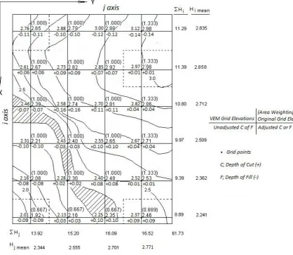
Land Grading According to Its Natural Slope (Application 2)
In order to test the performance of the developed method (VEM), land grading calculations were performed in the same area according to its natural slope values. The calculations were performed for a cut/fill ratio between 1.15 and 1.25 assuming the land had light textured soil (Table 1) and for a natural slope value in X and Y directions based on the natural elevations of the land (Figure 3). For the comparison of VEM results, the land grading calculations were also performed for the current methods, LSM and SRM on the same area and the results obtained are summarized in Table 3. In each of the three methods applied in this study the natural slope is identified different ways. Because of that, natural slopes in X direction for LSM, SRM and VEM methods were –0.450%, – 0.483%, and –0.396% respectively (Table 3).
Similarly, natural slopes in Y direction for LSM, SRM and VEM methods were 0.483%, 0.483%, and 0.474%, respectively. Even if different values were obtained for each of the three methods, natural slope was found negative in X direction and positive in Y direction. The proposed VEM method gives a slightly low natural slope than LSM and SRM methods. Considering the terms of surface irrigation, on the condition that the slope is within the limits of the irrigation method to be applied, the low slope value is desirable especially in terms of soil erosion. According to the unbalanced grading results; the total cut volumes for LSM, SRM, and VEM methods were found 339.0, 288.0, and 822.0
m3, respectively. The total fill volumes obtained in LSM, SRM
and VEM methods were 1,367.9, 1,459.9, and 545.0 m3,
respectively.
Table 3. Grading calculations in X and Y directions with natural slope
Features Methods
Least Square Method (LSM)
Symmetric Residuals Method (SRM)
Volume Equalization Method (VEM)
Natural slope in X direction, % –0.450 –0.483 –0.396
Natural slope in Y direction, % 0.483 0.483 0.474
UB* Total cut volume, m3 339.0 288.0 822.0
Total fill volume, m3 1367.9 1459.9 545.0
Cut/ fill ratio 0.248 0.197 1.508
B* Total cut volume, m3 730.0 808.0 729.0
Total fill volume, m3 653.9 653.9 673.0
Cut/ fill ratio 1.120 1.223 1.080
Cut volume per hectare, m3ha-1 330.3 365.6 329.9
UB; unbalanced results, B; balanced results
Accordingly, the cut/fill ratios in LSM, RSM, and VEM methods were 0.248, 0.197, and 1.508, respectively. According to the balanced grading results, the total cut volumes obtained for LSM, SRM, and VEM methods were
730.0 m3, 880.0 m3 and 729.0 m3, respectively. Similarly, the
total fill volumes for the three methods (LSM, SRM and
VEM) were 653.9 m3, 653.9 m3 and 673.0 m3, respectively.
The cut/fill ratio values in the same order were 1.120, 1,223, and 1.080. Here, the cut/fill ratio values of LSM and VEM methods remained slightly below the required limit (1.15 to 1.25). This is why the balancing process is carried out on the basis of cm for all methods. If the height of the grading plane is lowered by 1 cm during the balancing process, the cut/fill ratio value rises above the upper limit value (1.25). Therefore, the values obtained (1.12 and 1.08) are accepted as appropriate. On the other hand, the volumes of cut per hectare
were found 330.3 m3, 365.6 m3 and 329.9 m3 in LSM, SRM,
and VEM methods, respectively. According to the land grading calculations for natural slope in two directions, the total cut volume values of the three different methods are almost equal, and it can be said that VEM method gives as accurate results as LSM and SRM methods which are in practice. There is a minor difference between the methods and the reason for that difference is the cut/fill ratios of the methods. If not taken into account the difference between cut/fill ratios of the methods, it is understood that the cut volume per hectare for all methods is very close to each other.
Conclusions
This study presents “uniform sloped land grading in two directions of the Volume Equalization Method (VEM)” newly developed for land grading design, and it can be seen as continuation of “uniform sloped land grading in one direction developed by Y. Ayranci and K.E. Temizel (2011). The method is based on the principle “the soil should not be
brought from another place to the land grading area nor should it be removed from the land grading area”. Hence, the
soil volumes before and after grading measured from a reference elevation are equal. In this study, the mathematical principles of the VEM for uniform sloped land grading in two directions are presented and land grading for its natural slope in two directions and the method has been tested in a hypothetical area covering 2.21 ha. In order to assess the VEM results, LSM and SRM methods were also applied to the same area. According to the results, the VEM is as accurate as the conventional methods, Least Squares Method (LSM) and Symmetric Residuals Method (SRM) in rectangular fields.
REFERENCES
Ayranci, Y., and K.E. Temizel. 2011. Volume equalization method for land grading design: Uniform sloped grading in one direction in rectangular fields. African Journal of
Biotechnology 10(21):4412–4419.
Chugg, G.E. 1947. Calculations for land gradation.
Agricultural Engineering 28(11): 461–463.
Easa, S.M. 1989. Direct land grading design of irrigation plane surfaces. Journal of Irrigation and Drainage Engineering 115(2): 285–301.
Gebre-Selassie, N. A., and L.S. Willardson. 1991. Application of Least Squares land leveling. Journal of Irrigation and
Drainage Engineering 117(6): 962–966.
Givan, C.E. 1940. Land grading calculations. Agricultural
Engineering 21(1):11–12.
Hamad, S.N., and A.M. Ali. 1990. Land Grading design by using nonlinear programming. Journal of Irrigation and
Drainage Engineering 116(2):219–226.
Harris, W.S., J.C. Wait, and R.H. Benedict. 1966. Warped surface method of land grading. Transsection of American
Society of Agricultural Engineers 9(1):64–65.
James, L.G. 1988. Principles of Farm Irrigation System Design. Singapore, John Wiley&Sons, Inc. p. 336 – 340. Marr JC (1957). Grading land for surface irrigation. Circular
438. Univ. of California, Agric. Exp. Sta. Services.
Raju, V.S. 1960. Land grading for irrigation. Transsection of
American Society of Agricultural Engineers 3(1):38–41.
Scallopi, E.J., and L.S. Willardson. 1986. Practical land grading based on least squares. Journal of Irrigation and
Drainage Engineering 112(2):98–109.
Shih, S.P., and G.J. Kriz. 1971. Symmetrical residuals methods for land forming design. Transsection of
American Society of Agricultural Engineers 14(6):1195–
1200.
Srinisava, L.R. 1996. Optimal land grading based on genetic
algorithms. Journal of Irrigation and Drainage
Engineering 122(4):183–188.
Walker, W.R. 1989. http://www.fao.org/docrep/T0231E/ T0231E00.htm.
Yildirim, O. 2008. Sulama Sistemlerinin Tasarımı. Ankara, Turkey: Ankara University Printing House. (In Turkish). Zimmermann, K.R., A. Gross, M., O’Connor, G., Sapilevski,
D.G., Lawrence, H.S., Cobb, L. Leckie, and P.Y. Montgomery. 2005. System and Method for Land Leveling United States Patent No: US-6,880,643-B1.