Global ray-casting range image registration

R E S E A R C H P A P E R

Open Access

Global ray-casting range image

registration

Linh Tao

, Tam Bui

and Hiroshi Hasegawa

Abstract

This paper presents a novel method for pair-wise range image registration, a backbone task in world modeling, parts inspection and manufacture, object recognition, pose estimation, robotic navigation, and reverse engineering. The method finds the most suitable homogeneous transformation matrix between two constructed range images to create a more complete 3D view of a scene. The proposed solution integrates a ray casting-based fitness estimation with a global optimization method called improved self-adaptive differential evolution. This method eliminates the fine registration steps of the well-known iterative closest point (ICP) algorithm used in previously proposed methods, and thus, is the first direct global registration algorithm. With its parallel implementation potential, the ray

casting-based algorithm speeds up the fitness calculation for the global optimization method, which effectively exploits the search space to find the best transformation solution. The integration was successfully implemented in a parallel paradigm on a multi-core computer processor to solve a simultaneous 3D localization problem. The fast, accurate, and robust results show that the proposed algorithm significantly improves on the registration problem over state-of-the-art algorithms.

Keywords: Range image registration, Direct global registration, Adaptive differential evolution, Global optimization, Ray-casting, 3D localization

1 Introduction

The introduction of commercial depth sensing devices, such as the Microsoft Kinect and Asus Xtion, has shifted the research areas of robotics and computer vision from 2D-based imaging and laser scanning toward 3D-based depth scenes for environment processing. As physical objects or scenarios are built using more than a single image, images from different times and positions need to be aligned with each other to provide a more complete view. We call the alignment process registration, and it plays a key role in object reconstruction, scene mapping, and robot localization applications. Depending on the number of views that are processed simultaneously, regis-tration is divided into multi-view [1] and pair-wise cases [2]. Our paper focuses on the latter case for constructed range images captured by 3D cameras. From two images, called the model and the data, the registration algorithm finds the best homogeneous transformation that aligns

*Correspondence: [email protected]

1_{Department of Functional Control System, Shibaura Institute of Technology,} 307 Fukasaku, Minuma-ku, Saitama City, Saitama, 337-8570, Japan Full list of author information is available at the end of the article

the data and the model image in a common coordinate system.

The iterative closest point (ICP) algorithm [3] and its variants, such as EM-ICP [4] and generalized ICP [5], have been indispensable tools in registration algorithms. ICP’s concept and implementation are easy to understand. It derives a transformation that draws images closer to each other using theirL2error iteratively. ICP-class algo-rithms have a drawback for general registration in that they require a further assumption of near-optimal initial pose transformation; otherwise, the registration process is likely to converge to local instead of global or near global optima. Some mesh and point cloud editor software programs, such as Meshlab [6], include an ICP built-in registration tool; however, they require that users perform manual pre-alignment before ICP can be applied.

To overcome the shortage of ICP-class methods, auto-matic registration algorithms in general perform two steps: coarse initialization and fine transformation. If two point clouds are sufficiently close, the first step can be omitted. Otherwise, researchers are faced with

a big challenge. Two approaches for coarse transforma-tion, pre-alignment estimatransforma-tion, or initialization exist: local and global. The former uses local descriptors (or sig-natures), such as PFH [7] and SIFT [8], which encode local shape variation in neighborhood points. If the key points of these descriptors appear in both registered point clouds, the initialization movement can be estimated by using sample consensus algorithms, such as RANSAC [9]. Unfortunately, it is not always guaranteed that these sig-natures will appear in both registered point clouds. On the other hand, global approaches, such as Go-ICP [10] and SAICP [11], take all the points into account. The com-putation cost is the biggest problem in this approach. In big number data cases, the computation cost becomes large. By virtue of new search algorithms, in particular heuristic optimal methods, and the increase in computer speed achieved by using multi-core computer processor units (CPUs) and graphic computation units (GPUs) [12], it is possible to find reasonable solutions using global approaches for the registration problem. When the coarse transformation has been estimated, the ICP algorithm is an efficient tool for finding the fine transformation.

By integrating optimal search tools with an ICP algo-rithm, researchers have created hybrid algorithms that integrate global optimizers with ICP. However, this approach has its limitations. SAICP, a parameter-based algorithm, uses simulated annealing (SA) [13] as a search engine to find the best movement combination of rota-tion angles and translarota-tion. However, SA is not sufficiently effective to allow its application to a complicated fitness function, where the potential of a failed convergence is high. Go-ICP converges slowly, since it uses the branch-and-bound (BnB) method, a time consuming and non-heuristic method, as a search algorithm to ensure a 100% convergence rate. In addition, ICP algorithms frequently include a kd-tree structure for searching corresponding points. Using the kd-tree nearest neighbor search method also leads to a high computation cost and a long runtime.

In this paper, a new global direct registration method for 3D constructed surfaces captured by range cameras in cases where the initialization is not good is proposed.

- It eliminates the ICP algorithm from the registration process and thus becomes a direct method.

- As other global registration methods, the new method requires no local descriptors and operates directly on raw scanning data.

- The method uses the improved self-adaptive differential evolution (ISADE) algorithm [14] as a search engine to find the global minima as a direct method that does not use a fine registration procedure such as ICP.

- Furthermore, ray casting-based error calculation reduces the computation cost and runtime because

of the potential for using parallelized computation. CPU-based parallel computing procedures allow the algorithm to find the solution at a rate equivalent to the online rate.

The structure of this paper is as follows.

- Section 1 comprises the introduction.

- In Section 2, the classic and up-to-date methods of range image registration are presented.

- In Section 3, the methodology and the new approach of the proposed method are provided.

- In Section 4, the experiments and results are described.

- In Section 5, the discussion and conclusions are presented.

2 Range image registration

This part summarises some approaches for global range image registration problem up to date.

2.1 Registration error function and ICP approach

SVD and PCA [15] are integrated with ICP in classical methods and global search algorithms are integrated with ICP in most current hybrid methods. In this integration, SVD and PCA find the coarse transformation while ICP is the fine transformation estimation tool. The original ver-sion of the ICP algorithm relies on theL2error to derive the transformation (rotation R ∈ SO3 and translation t∈R3), which minimizes theL2type error:

E(R,t)= n

i=1

ei(R,t)= n

i=1

|Rxi+t−yj∗| (1)

where X = {xi},{i = 1, 2, 3,. . .,m} is the model point

cloud andY = {yj},{j = 1, 2, 3,. . .,n}is the data point

cloud, xi andyj ∈ R3 are the coordinates of the points

in the point clouds,Randtare the rotation and transla-tion matrix, respectively,yj∗is the corresponding point of xidenoting the closest point in data point cloudY.Rand t are determined by Roll-Pitch-Yaw movement of three rotation angles(α,β,γ )and translation values(x,y,z).

Variants of the ICP algorithm rely on different distance categories to define the closest points. Point-to-point dis-tance and point-to-plane disdis-tance are two popular exam-ples. Equation 2 presents the former case.

j∗=argmin j∈{1,...,n}

||Rxi+t−yj|| (2)

The following iterative process is designed to achieve the final transformation.

1. Compute the closest model points for each data point as in Eq. 2.

3. ApplyRandtto the data point clouds.

4. Repeat steps 1, 2, and 3 until the error obtained using (1) is smaller than a set tolerance level or the

procedure reaches its maximum iteration.

Step by step, the data point cloud becomes closer to the model point cloud and the process stops at local minima. ICP’s variants, such as LMICP [16] and SICP [17], use dif-ferent methods to calculate the transformation from error E(R,t). A well-known accumulation registration method in the KinectFusion algorithm [18] uses ICP to register two consecutive frames. The transformation matrix for the current frame is estimated by multiplying the matrices from the previous registration steps.

2.2 Global hybrid registration algorithm

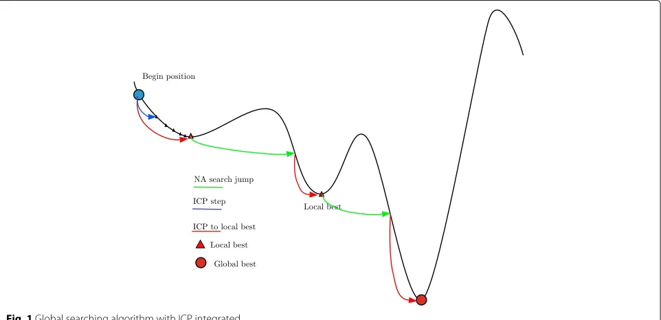
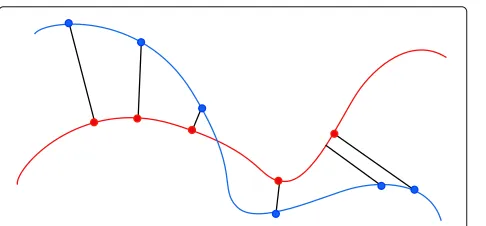
ICP algorithms constitute the most suitable method for registering close or pre-aligned point cloud data. In other cases, the algorithm frequently converges incorrectly. Global search algorithms are suitable for solving this prob-lem, since they can find the global instead of the local minima. To reduce the burden of the global search algo-rithm, researchers frequently flatten the search space by using ICP. Figures 1 and 2 show an example of ICP’s oper-ation as a flattening tool. In Fig. 1, from any beginning point, after many iterations, ICP finds the nearest local optima point. Figure 2 shows that a complex fitness func-tion (colored black) becomes a simpler one (colored red). As a result, global search methods are able to find the global minima more effectively.

The integration is effective in the case of point cloud data where the point number is small. For cases where

the point number is large, the hybrid approach with ICP becomes slow. This method cannot therefore be imple-mented in real-time applications.

3 The new direct global approach

With the newly developed global search algorithms, flat-tening using ICP inner loops in registration becomes redundant. Our method integrates a new global search algorithm, ISADE, which is suitable for complicated fit-ness functions when the flattening process is not per-formed, and a ray casting-based corresponding search method to accelerate the objective function calculation in the registration procedure.

3.1 Ray-casting for fast corresponding point determination on constructed range image

The KinectFusion algorithm, a real-time scene recon-structing pipeline, uses ICP as the only method for regis-tering two continuous frames. The procedure requires a powerful GPU to speed up calculations and reduce run-time. However, global registration algorithms calculate a thousand times more error functions than ICP and thus, so that these algorithms can be applied online or using less powerful processors, faster error calculation methods must be included.

ICP algorithms use the kd-tree [19] structure to speed up the process of determining j∗ in Eq. 2. The com-plexity of the kd-tree nearest neighbor search algorithms is O(log(n)), where n is the set number of the search points. Figure 3 shows an example of the true clos-est corresponding points of the model and data point clouds.

Fig. 2Example of flatten objective function after ICP inredcolor where original function is inblack

Ray casting [20] is one of the most basic of the many computer graphics rendering methods. The idea behind the ray-casting method is to direct a ray from the eye through each pixel and find the closest object blocking the path of the ray. Using the material properties and light effect in the scene, rendering methods can determine the shading of the object. Some hidden surface removal algo-rithms use ray casting to find the closest surfaces to the eye and eliminate all others that are at a greater distance along the same ray. The Point Cloud Library [21] uses ray casting as a filtering method; it removes all points that are obscured by other points.

We apply ray casting to find the approximated clos-est point using a range camera model. Constructed range images or point cloud data are frequently captured by a 3D range camera, where a range image can be consid-ered a 2D gray image,G; the value of each pixel shows the depth of a point. To simplify the problem, we do not take distortion into consideration.

zi,j=Gi,j (3)

wherezi,jis the depth of the image at pixel columniand

rowj.

Fig. 3Closest corresponding point using kd-tree. Data points are in blueand model points are inred

Equation 4 converts range image data points to real 3D depth data{x,y,z}inR3.

xi,j=(i−cx)Gi,j/fx (4a)

yi,j=(j−cy)Gi,j/fy (4b)

zi,j=Gi,j (4c)

wherefx,fy,cx, andcyare the intrinsic parameters of the depth camera.

Inversely, pixel positioni,jis to be calculated. Figure 4 shows the method’s idea.

Using the corresponding points obtained in the ray-casting step, we determine the depth differencezi,jfor

the next step of calculating the objective function for the global search method, as

zi,j(R,t)=

zX_i,j−zY_i,jR,t

0 if

|zi,j(R,t)|<thresthold

otherwise

(5)

where R and t are the rotation and translation matrix, respectively,zX_i,jis the depth of the model point cloud, and

z_iY_,j(R,t)is the depth of the data point cloud after applying the rotation and translation matrix withi,jfrom the ray casting process.

The ray-casting method is simple and fast (with a com-plexity ofO(1)) and, more importantly, potentially parallel computing can be applied.

3.2 Objective function

Global optimization methods use fitness or objective functions to find the transformation that drives the fit-ness function to the smallest value. We propose a fitfit-ness functionF(R,t):

F(R,t)= f(k)1 k2

n

i=1 m

j=1

(zi,j(R,t))2 (6)

where R and t are the rotation and translation matrix, respectively,mandnare the height and width of the image frame, andkis the inlier point number.

To gain a smaller error in a larger number of inlier points, we used an additional functionf(k):

f(k)=

∞ 1−k/Nif

k<N/10 kN/10

(7)

whereNis the number of points in the data point cloud. The ray-casting-based method makes the algorithm run significantly faster than the kd-tree-based approach. However, since a global search algorithm handles a large number of points at a huge computation cost, we take parallel implementation into consideration. Since in most computers a multi-core processor is available, using the CPU for parallel computing is convenient in most applications. In addition, CPU multi-core parallel imple-mentation is even easier with OpenMP library [22]. Fur-thermore, the ray-casting process adapts well to parallel computing, and the corresponding points can be calcu-lated in different processes or threads.

3.3 ISADE, an efficient improved version of differential evolution algorithm

3.3.1 Differential evolution

Differential evolution (DE) is an evolutionary opti-mization technique originally proposed by Storn and Price [23], characterized by operators of mutation and crossover. In DE, the scaling factorFand crossover rateCr

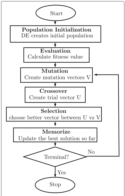
determine the correction and speed of convergence, while another important parameter, NP, the population size, remains a user-assigned parameter to handle problem complexity. Figure 5 shows pseudo-code or implementa-tion flowchart of DE algorithms.

a) Initialization in DEThe initial population was gen-erated uniformly at random in the range lower boundary (lb) and upper boundary (ub).

X_iG=lbj+randj(0, 1)(ubj−lbj) (8)

where randj(0, 1)a random number∈[ 0, 1].

b) Mutation operationIn DE, there are various mutation schemes to create mutant vectorsV_iG = V_iG_,1,. . .,V_iG_,D for each individual of population at each generation G. XG_i is target vector in the current population,Dis vector dimension number.

DE/rand/1 :V_iG_,j =X_rG_1,j+F XG_r2,j−X_rG_3,j (9a)

DE/best/1 :V_iG_,j =X_best,G _j+F X_rG_1,j−X_rG_2,j (9b)

Fig. 5DE implementation process

DE/currenttobest/1:V_iG_,j=X_iG_,j+F X_best,G _j−X_iG_,j

+FX_rG_1,j−XG_r2,j

(9c)

DE/rand/2 :V_iG_,j =X_iG_,j+F X_rG_2,j−X_rG_3,j

+F X_rG_4,j−X_rG_5,j

(9d)

DE/best/2 :V_iG_,j=X_best,G _j+F X_rG_1,j−X_rG_2,j

+F X_rG_3,j−X_rG_4,j

(9e)

DE/randtobest/1:V_iG_,j=X_best,G _j+FX_best,G _j−XG_r2,j

+FX_rG_2,j−X_rG_3,j

(9f)

c) Crossover operationAfter mutation process, DE per-forms a binomial crossover operator on X_iG andV_iG to generate a trial vector U_iG = U_iG_,1,. . .,U_iG_,D for each individual populationias shown in Eq. 10.

U_iG_,j =

V_iG_,j if randjCr or j=jrand X_iG_,j otherwise

(10)

where i = 1,. . .,NP, j = 1,. . .,D , jrand is a ran-domly chosen integer in [ 1,D] , randj(0, 1)is a uniformly

distributed random number between 0 and 1 generated for eachjandCr ∈[ 0, 1] is called the crossover control

parameter. Usingjrandensures the difference between the trial vectorU_iGand target vectorX_iG.

c) Selection operation The selection operator is per-formed to select the better solution between the target vector X_iG and the trial vector U_iG entering to the next generation.

X_iG+1=

U_iG if f(U_iG)f(X_iG) X_iG otherwise

(11)

wherei = 1,. . .,NP,XG_i +1is a target vector in the next generation’s population.

3.3.2 Improvement of self-adapting control parameters in differential evolution

a) Adaptive selection learning strategy in mutation opera-torIn our study of ISADE, we randomly chose three muta-tion schemes: DE/best/1/bin, DE/best/2/bin, and DE/rand to best/1/bin. DE/best/1/bin and DE/best/2/bin have a good convergence property, and DE/rand to best/1/bin has a good population diverse property. The probability of applying these strategies is equal at values ofp1 = p2 = p3=1/3.

DE/best/1 :V_iG_,j =X_best,G _j+F XG_r1,j−X_rG_2,j

(12a)

DE/best/2 :V_iG_,j=X_best,G _j+F X_rG_1,j−X_rG_2,j+F X_rG_3,j−XG_r4,j (12b)

DE/randtobest/1:V_iG_,j=X_best,G _j+FX_best,G _j−X_rG_2,j

+FX_rG_2,j−X_rG_3,j

(12c)

wherer1,r2,r3,r4, andr5are randomly selected integers in the range [ 1,NP], whereNPis the population size.

b) Adaptive scaling factor To achieve a better perfor-mance, ISADE gives the scale factorFa large value initially to allow better exploration and a small value after the generations to allow appropriate exploitation. Instead of using sigmoid scaling in Eq. 13 taken from Tooyama and Hasegawa’s study on APGA/VNC [24], ISADE adds a new factor to calculateFas shown in Eq. 14.

Fi =

1

1+exp α∗i−_NPNP/2

(13)

Fi =

Fi+Fimean

2 (14)

in whichF_imeanis calculated as Eq. 15.

F_imean=Fmin+(Fmax−Fmin)

imax−i imax

niter

(15)

whereFmaxandFmindenote the lower and upper bound-ary condition of Fwith recommended values of 0.8 and 0.15, respectively.i,imax, andniterdenote the current, max generation, and nonlinear modulation index as in Eq. 15.

niter=nmin+(nmax−nmin)

i imax

(16)

where nmax and nmin are typically chosen in the range [ 0, 15]. Recommended values for nmin andnmax are 0.2 and 6.0 respectively.

c) Crossver control parameter ISADE is able to detect whether the height of Cr values are useful. The control

parameterCris assigned as

C_ri+1=

rand2 if rand1τ Ci_r otherwise

(17)

where rand1and rand2are random values∈[ 0, 1] ,τ rep-resents the probability to adjustCr, which is also updated

using

C_ri+1=

Crmin CrminCri+1Crmedium Crmax CrmediumCri+1Crmax

(18)

whereCrmin,Crmedium, andCrmaxdenote a low value, median value, and high value of the crossover parameter, respec-tively. We use recommended values ofτ = 0.1,Crmin = 0.05,Crmedium =0.50, andCrmax=0.95.

d) Combination of ISADE and ray-castingISADE elimi-nates tuning tasks for the problem-dependent parameters F and Cr. With simple adaptive rules, the

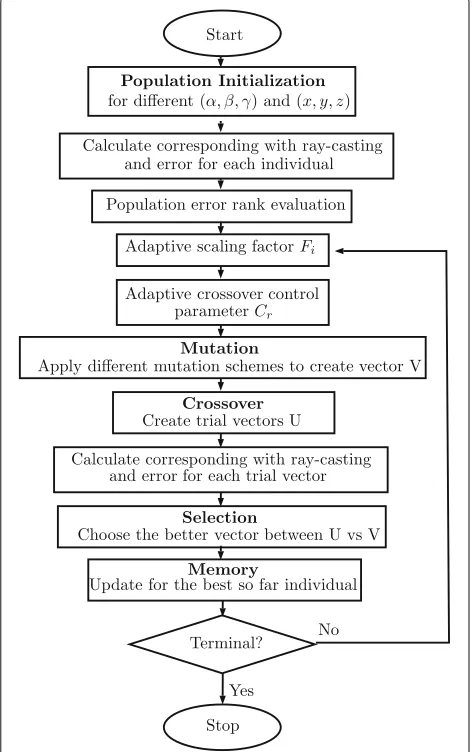
computa-tion complexity of this new version of the DE algorithm remains the same as that of the original version. All the above ideas and theories of ISADE algorithm and ray-casting method are implemented as in the flowchart shown in Fig. 6.

4 Experiment and results

This section describes experiments that were conducted using the proposed method in real range image data reg-istration and presents the results. We integrated different global search methods with the ray casting-based algo-rithm in order to obtain a comparison between ISADE and the state-of-the-art methods as follows.

Fig. 6ISADE implementation process with ray-casting corresponding method

2) Particle swarm optimization (PSO) proposed in Talbi et al.’s paper, Particle swarm optimization for image processing [25].

3) Genetic algorithm (GA) proposed in Valsecchi et al.’s paper, An image registration approach using genetic algorithms [26].

4) DE proposed in Falco et al.’s paper, Differential evolution as a viable tool for satellite image registration [27].

We also calculated the ray casting-based error of the KinectFusion and Go-ICP algorithms for further com-parison. All algorithms were implemented in C++ and compiled with GNU/g++ tool.

4.1 Range image dataset

In our experiments, a number of pair-wise registra-tions was conducted using well-known depth data,

“RGB-D Dataset 7-Scenes,” taken from the Kinect Microsoft Camera downloaded from the Microsoft Research Website, http://research.microsoft.com/en-us/ projects/7-scenes/. Specifically, Figs. 7 and 8 show all the scenes: Chess, Fire, Heads, Office, Pumpkin, RedKitchen, and Stairs. The details of the data used in the registration experiments are as follows.

Chess dataset: image sequence 2, frame 960 vs frame 980.

Other datasets: image sequence 1, frame 000 vs frame 020.

These “PNG” format depth images are sub-sampled into a smaller resolution of 128 × 96, which is five times smaller than the original resolution of 640×480 in each dimension. The purpose of using a dataset with a smaller number of points is to achieve a suitable runtime while preserving robustness and accuracy.

4.2 Parameter settings

For each method, 30 runs were performed. The search space had rotation angles and translation limited at [−π/5,π/5] and [−1, 1] separately. This means that the limitation of the rotation angles was 36◦and of the trans-lation was 1 m.

The algorithm parameters shown in Table 1 constitute the configuration for all the algorithms. All methods were run on a desktop PC powered with an Intel core I7-4790 CPU 3.60 GHz× 8 processor, 8 GB RAM memory and Linux Ubuntu 14.04 64-bit Operation System. The new algorithm C++ code was written based on reference from Andreas Geiger’s LIBICP code [28].

4.3 Comparison with KinectFusion algorithm

Accompanied by depth ranger images, “RGB-D Dataset 7-Scenes” provides homogeneous camera to world trans-poses at each frame calculated using the KinectFusion algorithm. We converted those camera transposes into transformation matrix between two frames as

T_ij=T_i−1∗Tj (19a)

T_ij=

⎡ ⎢ ⎢ ⎣ R

j i t

j i

0 0 0 1

⎤ ⎥ ⎥

⎦ (19b)

whereT_ijis the transformation matrix to move framejto align with framei,TiandTjare the homogeneous

Fig. 7RGB-D Chess, Fire, Heads, Office dataset for experiments

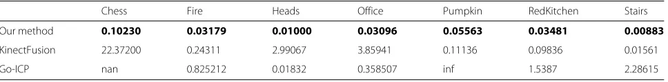
Rj_i and tj_i are applied to ray-casting error calculation methods for two frames, as in Eq. 6, to describe the errors of the KinectFusion algorithm. Table 2 presents the mean errors of the proposed method in comparison with the error of the KinectFusion algorithm. The signifi-cantly smaller mean errors of the proposed method prove its superiority to the KinectFusion algorithm registration pipeline.

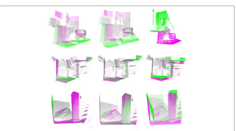
Figures 9 and 10 visually show the registration results of the proposed algorithm for the seven scenes in center and those of KinectFusion on the left hand

side, to provide a visual comparison. The seven scenes included are Chess, Fire, Heads, Office, Pumpkin, Red-Kitchen, and Stairs. The model point clouds are col-ored red, and the data point clouds are colcol-ored green.

In these figures, the proposed algorithm outperforms KinectFusion is clearly seen. Even in the best case of KinectFusion, such as Stairs or RedKitchen, the overlapping regions, where the two colors are mixed together, are not as clearly seen as in the results of the proposed algorithm.

Table 1Algorithm configuration

Algorithm DE GA SA PSO Go-ICP

Parameters F0=0.8 Pc=0.95; α=0.995 elites=4 trimFraction=0.0

Cr=0.9 Pm=0.1; neighbors=5

DE/rand/1/bin elites=5 c1=c2=c3=2.1 distTransSize=50

Maxgen 100 100 3000 100;

Population 30 30 30 data subsample=1000 points

An example of applying the new method to consec-utive localizations can be seen in Fig. 11. The pump-kin 3D scene, which is built from seven different range images (frame 000, 020, ..., 120), visually shows the accu-racy of the proposed method at various percentages of overlapping regions. The different frames are in differ-ent colors. A video at https://www.youtube.com/watch?v= sgaUry5qsxU gives a clearer view.

4.4 Comparison with Go-ICP algorithm

From authors contributed code [29], we performed exper-iments to compare our method with Go-ICP on accu-racy, runtime, and robustness. Go-ICP configuration parameters were set as in Table 1 with the identical searching boundary with other methods. distTransSize is the number of nodes in translation searching bound-ary. It was set to 50 or translation resolution is at 40 mm. Raising accuracy by increasing distTransSize to 500 or 4 mm resolution effort failed due to infinite run-time. Go-ICP were able to register Heads and Office datasets at distTransSize of 100 with runtime presented in Table 5.

The disadvantage of big resolution could be compen-sated by inner ICP loops; however, the smaller the resolu-tion, the more accurate the algorithm is. We set the data subsample to 1000; Go-ICP reaches infinitive runtime at the original 128×96 resolution.

Together with KinectFusion and our method errors, Table 2 presents the mean errors of Go-ICP algorithm where “nan” stands for undefined result in the case of infinitive runtime and “inf ” stands for wrong convergence with few overlapse points. Over all, only heads and office showed good convergence with small error and run time. However, those small errors are still bigger than the new method.

Figures 9 and 10 also show the registration results of Go-ICP algorithm on the right side together with new method results in the center and KinectFusion algorithm result on the left side. From those figures, the new method bet-ter performance is clearly seen. In the case of RedKitchen dataset, the wrong convergence results of Go-ICP were observed, the error was small because of small over-lapsed percentage.

Average runtime for Go-ICP on different datasets are presented in Table 5 where average run times of the new algorithm at different generation numbers are presented. In the table, “inf ” values stand for infinitive runtime. Go-ICP was fast in case of heads dataset or extreme slow for the case of Chess dataset.

Over all, the new methods outperformed Go-ICP on experiment datasets in accuracy, runtime, and robustness.

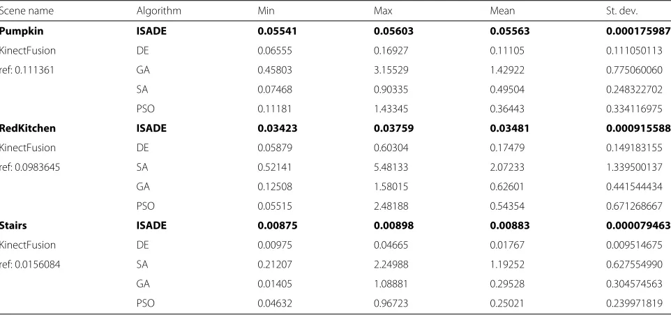
4.5 Comparison between different optimization algorithms

Tables 3 and 4 show the experimental results of all the integrations and methods in four categories: min, max, mean, and standard deviation.

The smaller means and standard deviations for every dataset in comparison with the other methods show the accuracy and robustness of the new search engine as com-pared to the state-of-the-art search algorithms. In some cases, the experimental results show that the other inte-grations performed better than KinectFusion. The ICP accumulating error is the reason for this poor perfor-mance.

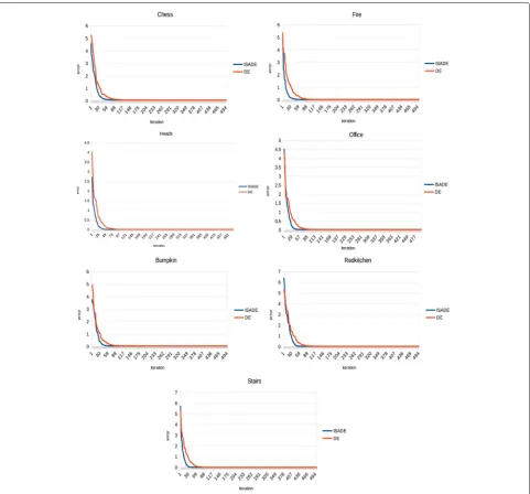
4.6 Iterations vs convergence

In Fig. 12, we compare the robust results of conver-gence of the registration of the seven scenes for a small number of iterations between using ISADE and

Table 2Error comparison between new method, KinectFusion, and Go-ICP algorithms

Chess Fire Heads Office Pumpkin RedKitchen Stairs

Our method 0.10230 0.03179 0.01000 0.03096 0.05563 0.03481 0.00883

KinectFusion 22.37200 0.24311 2.99067 3.85941 0.11136 0.09836 0.01561

Go-ICP nan 0.825212 0.01832 0.358507 inf 1.5387 2.28615

Table 3Results of Chess, Fire, Heads, and Office datasets

Scene name Algorithm Min Max Mean St. dev.

Chess ISADE 0.10047 0.11187 0.10230 0.002821482

KinectFusion DE 0.17453 3.92808 0.29860 0.112087291

ref: 22.372 GA 1.44923 1.80180 2.53723 0.691936150

SA 1.11736 2.55157 1.65871 0.400817542

PSO 1.19899 2.58186 1.72316 0.459892382

Fire ISADE 0.03169 0.03196 0.03179 8.70855E−005

KinectFusion DE 0.03873 0.26059 0.10263 0.066038287

ref: 0.243112 GA 0.22177 3.93133 1.58268 0.913837133

SA 0.15060 0.88670 0.45855 0.249700426

PSO 0.11158 0.63419 0.34592 0.151824890

Heads ISADE 0.00994 0.01016 0.01000 7.01799E−005

KinectFusion DE 0.01276 0.06570 0.02205 0.012768061

ref: 2.99067 GA 0.47056 1.70316 0.97758 0.358190303

SA 0.30740 1.01428 0.65404 0.264058658

PSO 0.20801 1.88772 0.54401 0.463097716

Office ISADE 0.03084 0.03115 0.03096 8.39925E−005

KinectFusion DE 0.03195 0.06436 0.04373 0.009462166

ref: 3.85941 GA 0.24518 4.05346 1.88819 0.928751342

SA 0.10385 2.67972 0.84426 0.720046753

PSO 0.07169 2.08078 0.58507 0.686244921

The boldface entries are for emphasis for better result in comparison between the new method with other methods

DE, where the horizontal axis represents the iteration, and the vertical axis represents the error. In compar-ison with ISADE, DE required significant larger iter-ation number to achieve convergence. With ISADE, from 70 iterations, all the results show a flat trend

and no new optimal solutions with a significant dif-ference are found. This iteration number for DE is 120.

These results show that, if we reduce the maximum number of iterations to 70, the results remain the same.

Table 4Results of Pumpkin, RedKitchen and Stairs datasets

Scene name Algorithm Min Max Mean St. dev.

Pumpkin ISADE 0.05541 0.05603 0.05563 0.000175987

KinectFusion DE 0.06555 0.16927 0.11105 0.111050113

ref: 0.111361 GA 0.45803 3.15529 1.42922 0.775060060

SA 0.07468 0.90335 0.49504 0.248322702

PSO 0.11181 1.43345 0.36443 0.334116975

RedKitchen ISADE 0.03423 0.03759 0.03481 0.000915588

KinectFusion DE 0.05879 0.60304 0.17479 0.149183155

ref: 0.0983645 SA 0.52141 5.48133 2.07233 1.339500137

GA 0.12508 1.58015 0.62601 0.441544434

PSO 0.05515 2.48188 0.54354 0.671268667

Stairs ISADE 0.00875 0.00898 0.00883 0.000079463

KinectFusion DE 0.00975 0.04665 0.01767 0.009514675

ref: 0.0156084 SA 0.21207 2.24988 1.19252 0.627554990

GA 0.01405 1.08881 0.29528 0.304574563

PSO 0.04632 0.96723 0.25021 0.239971819

Fig. 9First four scenes (Chess, Fire, Heads, Office) registration output example. KinectFusion results are in thelefthand side, the new algorithm’s results are in thecenter, and Go-ICP algorithm’s results are on therighthand side

Fig. 11Office scene reconstructed results from different view angles

Clearly, the smaller the iteration number, the shorter is the runtime.

4.7 Results from registering in different movement patterns and frame distances

Figure 13 shows the values of rotation angles (α,β,γ) in radian and translation distances (x,y,z) in meter of 3D camera movement. Those values were obtained by using new algorithm to register range images from frame 001 to 060 respectively into the frame 000 of seq-01 in different datasets. The process stops if the movement val-ues get over searching boundaries. From all datasets, we choose three typical movement of Chess, Fire, and Heads

datasets for rotating, sliding, and forwarding with rotating movements respectively.

The results with no sudden value changing between two consecutive frames verify the feasibility of applying the new algorithm in registering range images of different movement patterns and frame distances.

4.8 Runtime

For the data of 128×96 resolution, average runtime for the proposed method are shown in Table 5. In the results, the average runtime for registration is around 0.6 s for 150 iterations of all scenes. Since the distance between two frames is 20, the registering equivalence rate is 33 frames

Table 5Average running time (in second) on different scenes of new methods and Go-ICP

New methods New method Go-ICP Go-ICP

100 generations 150 generations distTransSize = 50 distTransSize = 100

Chess 0.388414 0.516832 inf inf

Fire 0.385928 0.625765 14.2786 inf

Heads 0.335828 0.562451 0.102944 0.104659

Office 0.378768 0.560734 0.030326 34.411

Pumpkin 0.410615 0.621756 104.468 inf

RedKitchen 0.415258 0.588466 30.3815 inf

Fig. 12Fitness function as iterations of different datasets with ISADE inblueand DE inredcolor

per second (fps). At this rate, when we move the camera, the algorithm are able to update the scenarios.

By subsampling the data range image and remaining the model range image, the new algorithm gain smaller run-time while error level stays unchanged. Figure 14 shows the runtime at different level of subsample on the right hand and the errors in the left hand for the RedKitchen scenario.

5 Discussion

Image registration has become a very active research area. Recently, the approach of using EAs, in partic-ular in new methods, proved their potential for

tack-ling the image registration problem based on their robustness and accuracy for searching for global opti-mal solutions. When EAs are used as search tools, good initial conditions are not necessary for avoiding local minima while converging to near-global minima solutions.

Fig. 13Movement pattern from Chess, Fire, and Heads scenarios

A more important point is that, by eliminating inner ICP loops in hybrid integrations and fine-tuning procedures applied in previously proposed methods, the newly pro-posed method becomes the first direct, as well as the first online potential, global registration algorithm. Its robust-ness and accuracy were tested and verified in real 3D scenes captured by a Microsoft Kinect camera.

Currently, the algorithm is implemented using a CPU parallel procedure. In future work, the new algorithm can be implemented on a GPU to reduce its runtime and error while retaining its accuracy and robustness. Furthermore, the method can be extended for general point clouds from different sources by using a virtual camera surface and presenting it as a constructed surface. The proposed

method is also potentially suitable for super resolution range images.

Authors’ contributions

LT took charge of the system coding, doing experiments, data analysis and writing the whole paper excluding ISADE algorithm part at Subsection 3.3. TB took charge of coding and writing for ISADE algorithm part at Subsection 3.3. HH took charge of advisor position for paper presentation, experiment design, data analysis presentation as well English revising. All authors read and approved the final manuscript.

Competing interests

The authors declare that they have no competing interests.

Publisher’s Note

Springer Nature remains neutral with regard to jurisdictional claims in published maps and institutional affiliations.

Author details

1_{Department of Functional Control System, Shibaura Institute of Technology,}

307 Fukasaku, Minuma-ku, Saitama City, Saitama, 337-8570, Japan.2_{School of}

Mechanical Engineering, Hanoi University of Science and Technology, 1 Dai Co Viet Road, Ha Noi, Viet Nam.3_{Department of Machinery and Control System,}

Shibaura Institute of Technology, 307 Fukasaku, Minuma-ku, Saitama City, Saitama, 337-8570, Japan.

Received: 29 March 2016 Accepted: 12 April 2017

References

1. Sharp GC, Lee SW, Wehe DK (2004) Multiview registration of 3D scenes by minimizing error between coordinate frames. IEEE Trans Pattern Anal Mach Intell 26(8):1037–1050. doi:10.1109/TPAMI.2004.49

2. Holz D, Ichim AE, Tombari F, Rusu RB, Behnke S (2015) Registration with the Point Cloud Library: a modular framework for aligning in 3-D. IEEE Robot Autom Mag 22(4):110–124. doi:10.1109/MRA.2015.2432331 3. Besl P, McKay ND (1992) A method for registration of 3-d shapes. IEEE

Trans Pattern Anal Mach Intell 14(2):239–256. doi:10.1109/34.121791 4. Granger S, Pennec X (2002) Multi-scale EM-ICP: a fast and robust

approach for surface registration. In: European Conference on Computer Vision, vol. 2353. pp 418–432

5. Segal A, Haehnel D, Thrun S (2009) Generalized-ICP. In: Proceedings of Robotics: Science and Systems, Seattle, USA. doi:10.15607/RSS.2009.V.021 6. Meshlab. http://meshlab.sourceforge.net/. Accessed 15 Jan 2017 7. Rusu RB, Marton ZC, Blodow N, Beetz M (2008) Persistent point feature

histograms for 3D point clouds. In: Proceedings of the 10th International Conference on Intelligent Autonomous Systems (IAS-10), Baden-Baden. pp 119–128

8. Sehgal A, Cernea D, Makaveeva M (2010) Real-time scale invariant 3D range point cloud registration. In: Campilho A, Kamel M (eds). Image Analysis and Recognition. ICIAR 2010. Lecture Notes in Computer Science. Springer, Berlin Heidelberg Vol. 6111. doi:10.1007/978-3-642-13772-3_23 9. Wu F, Fang X (2007) An improved RANSAC homography algorithm for

feature based image mosaic. In: Proceedings of the 7th WSEAS International Conference on Signal Processing, Computational Geometry & Artificial Vision, ISCGAV’07, World Scientific and Engineering Academy and Society (WSEAS), Stevens Point, Wisconsin. pp 202–207. http://dl. acm.org/citation.cfm?id=1364592.1364627

10. Yang J, Li H, Jia Y (2013) Go-icp: Solving 3D registration efficiently and globally optimally. In: 2013 IEEE International Conference on Computer Vision, Sydney. pp 1457–1464. doi:10.1109/ICCV.2013.184

11. Luck J, Little C, Hoff W (2000) Registration of range data using a hybrid simulated annealing and iterative closest point algorithm. In: Proceedings 2000 ICRA. Millennium Conference. IEEE International Conference on Robotics and Automation. Symposia Proceedings (Cat. No.00CH37065), San Francisco Vol. 4. pp 3739–3744. doi:10.1109/ROBOT.2000.845314 12. Neumann D, Lugauer F, Bauer S, Wasza J, Hornegger J (2011) Real-time RGB-d

mapping and 3-D modeling on the GPU using the random ball cover data structure. In: 2011 IEEE International Conference on Computer Vision Workshops (ICCV Workshops), Barcelona. pp 1161–1167. doi:10.1109/ICCVW.2011.6130381

13. Ingber L (1993) Simulated annealing: practice versus theory. Math Comput Model 18(11):29–57. http://dx.doi.org/10.1016/0895-7177(93)90204-C 14. Bui T, Pham H, Hasegawa H (2013) Improve self-adaptive control

parameters in differential evolution for solving constrained engineering optimization problems. J Comput Sci Technol 7(1):59–74.

doi:10.1299/jcst.7.59

15. Marden S, Guivant J (2012) Improving the performance of ICP for real-time applications using an approximate nearest neighbour search. In: Proceedings of Australasian Conference on Robotics and Automation, New Zealand. pp 3–5

16. Lim Low K (2004) Linear least-squares optimization for point-toplane ICP surface registration. Tech Rep TR04-004, Department of Computer Science, University of North Carolina at Chapel Hill

17. Bouaziz S, Tagliasacchi A, Pauly M (2013) Sparse iterative closest point. In: Proceedings of the Eleventh Eurographics/ACMSIGGRAPH Symposium on Geometry Processing, SGP ’13, Eurographics Association. Aire-la-Ville, Switzerland. pp 113–123. doi:10.1111/cgf.12178

18. Izadi S, Kim D, Hilliges O, Molyneaux D, Newcombe R, Kohli P, Shotton J, Hodges S, Freeman D, Davison A, Fitzgibbon A (2011) Kinect-Fusion: real-time 3d reconstruction and interaction using a moving depth camera. In: Proceedings of the 24th Annual ACM Symposium on User Interface Software and Technology, UIST ’11. ACM, New York. pp 559–568. doi:10.1145/2047196.2047270

19. Chandran S (2012) Introduction to kd-trees. University of Maryland Department of Computer Science. https://www.cs.umd.edu/class/ spring2002/cmsc420-0401/pbasic.pdf

20. Roth SD (1982) Ray casting for modeling solids. Comput Graph Image Process 18(2):109–144. doi:http://dx.doi.org/10.1016/0146-664X(82)90169-1 21. Point cloud library. http://pointclouds.org/. Accessed 15 Jan 2017 22. Openmp. http://openmp.org/wp/. Accessed: 15 Jan 2017 23. Storn R, Price K (1997) Differential evolution a simple and efficient

heuristic for global optimization over continuous spaces. J Glob Optim 11(4):341–359. doi:10.1023/A:1008202821328

24. Tooyama S, Hasegawa H (2009) Adaptive plan system with genetic algorithm using the variable neighborhood range control. In: Evolutionary Computation, 2009. CEC ’09. IEEE Congress on Evolutionary Computation, CEC ’09. pp 846–853. doi:10.1109/CEC.2009.4983033 25. Chen YW, Mimori A, Lin C-L (2009) Hybrid particle swarm optimization for

3-d image registration. In: 16th IEEE International Conference on Image Processing (ICIP), Cairo. pp 1753–1756. doi:10.1109/ICIP.2009.5414613 26. Seixas FL, Ochi LS, Conci A, Saade DM (2008) Image registration using genetic algorithms. In: Proceedings of the 10th Annual Conference on Genetic and Evolutionary Computation, GECCO ’08. ACM, New York. pp 1145–1146. doi:10.1145/1389095.1389320

27. Falco ID, Cioppa AD, Maisto D, Tarantino E (2008) Differential evolution as a viable tool for satellite image registration. Appl Soft Comput 8(4):1453–1462. Soft Computing for Dynamic Data Mining. doi:http://dx. doi.org/10.1016/j.asoc.2007.10.013

28. Iterative closest point implementation C++ code. http://www.cvlibs.net/ software/libicp/. Accessed 15 Jan 2017