The block-constrained configuration model

R E S E A R C H

Open Access

The block-constrained configuration

model

Giona Casiraghi

Correspondence: [email protected] Chair of Systems Design, ETH Zürich, Weinbergstrasse 56/58, 8092 Zürich, Switzerland

Abstract

We provide a novel family of generative block-models for random graphs that naturally incorporates degree distributions: the block-constrained configuration model.

Block-constrained configuration models build on the generalized hypergeometric ensemble of random graphs and extend the well-known configuration model by enforcing block-constraints on the edge-generating process. The resulting models are practical to fit even to large networks. These models provide a new, flexible tool for the study of community structure and for network science in general, where modeling networks with heterogeneous degree distributions is of central importance.

Keywords: Block model, Community structure, Random graphs, Configuration model, Network analysis, gHypEG

Introduction

Stochastic block-models (SBMs) are random models for graphs characterized by group, communities, or block structures. They are a generalization of the classicalG(n,p) Erd˝os-Rènyi model (1959), where vertices are separated into Bdifferent blocks, and different probabilities to create edges are then assigned to each block. This way, higher probabili-ties correspond to more densely connected groups of vertices, capturing the structure of clustered graphs (Fienberg et al.1985; Holland et al.1983; Peixoto2012).

SBMs are specified by defining aB×Bblock-matrix of probabilitiesBsuch that each of its elementsωbibjis the probability of observing an edge between verticesiandj, wherebi denotes the block to which vertexibelongs. Most commonly, block-matrices are used to encode community structures. This is achieved by defining a diagonal block-matrix, with the inclusion of small off-diagonal elements.

Thanks to its simple formulation, the edge generating process of the standard SBM can retain the block structure of the graph that needs to be modeled (Karrer and Newman 2011). However, it fails to reproduce empirical degree sequences. The reason for this is that in theG(n,p)model and its extensions, edges are sampled independently from each other with fixed probabilities, generating homogeneous degree-sequences across blocks. This issue impairs the applicability of the standard SBM to most real-world graphs. Because of the lack of control on the degree distributions generated by the model, SBMs are not able to reproduce the complex structures of empirical graphs, resulting in poorly fitted models (Karrer and Newman2011).

Different strategies have been formulated to overcome this issue. Among others, one approach is that of using exponential random graph models (Krivitsky2012). These mod-els are very flexible in terms of the kind of patterns they can incorporate. However, as soon as their complexity increases, they lose the analytical tractability that character-izes the standard SBM. This is due to the need for computing the partition function that defines the underlying probability distribution (Park and Newman2004). Another, more prominent, approach taken to address the issue of uniform degree-sequences in SBMs are degree-corrected block models (DC-SBM) (e.g. Peixoto (2014); Newman and Peixoto (2015); Karrer and Newman (2011); Peixoto (2015)). Degree-corrected block-models address this problem by extending standard SBMs with degree corrections, which serve the purpose of enforcing a given expected degree-sequence within the block struc-tures. Moreover, this is achieved without hampering the simplicity of the standard SBM. For this reason, DC-SBMs are widely used for community detection tasks (Newman and Reinert 2016; Peixoto 2015). Recently, they have further been extended to a Bayesian framework, allowing non-parametric model estimation (Peixoto2017; Peixoto2018).

One of the main assumptions of G(n,p) models, SBMs, and DC-SBMs as well, is that the probability of creating edges for each pair of vertices are independent of each others (Kar-rer and Newman2011). While such a modeling assumption allows defining distributions whose parameters are in general easy to estimate, for many real-world graphs, this is a strong assumption that should be verified, and which is possibly unrealistic (Squartini et al.2015). Many social phenomena studied through empirical graphs, such as triadic clo-sure (Granovetter1973), or balance theory (Newcomb and Heider1958), are based on the assumption that edges between vertices are not independent. Similarly, for graphs aris-ing from the observation of constrained systems, like financial and economic networks, it is unreasonable to assume that edge probabilities are independent of each other. This is because the observed edges in the graph, which are the representation of interactions between actors in a system, are driven by optimization processes characterized by lim-ited resources and budget constraints, which introduce correlations among different edge probabilities (Caldarelli et al.2013; Nanumyan et al.2015).

Moreover, one of the consequences of the assumption of independence of edge proba-bilities is the fact that the total number of edges of the modelled graph is preserved only in expectation. In the case of SBMs and DC-SBMs, the total number of edges is assumed to follow a Poisson distribution. For a Poisson process to be the appropriate model for an empirical graph, the underlying edge generating process needs to meet the following conditions (Consul and Jain1973): (i) the observation of one edge should not affect the probability that a second edge will be observed, i.e., edges occur independently; (ii) the rate at which edges are observed has to be constant; (iii) two edges cannot be observed at precisely the same instant. However, it is often hard to evaluate whether these conditions are verified because the edge generating process may not be known, or these conditions are not met altogether.

Melnik et al. (2014) have proposed an alternative approach to the problem of preserving degree distributions and the independence of edges. Such an approach is a generalisation of the configuration model that allows constructing modular random graphs, charac-terised by heterogeneous degree-degree correlations between each block. The model, in particular, relies on specifying different valuesPbi,bi

bi. The so-calledPi,i

k,k-model, though, only considersunweightedandundirectedgraphs (Melnik et al.2014).

Similarly to the approach discussed in Melnik et al. (2014), we address the problem of incorporating degree distributions generalising the configuration model. Doing so, we propose a family of block-models that preserves the number of edges exactly, instead of in expectation. This circumvents the issue of assuming a given model for the number of edges in the graph, treating it merely as an observed datum. The configuration model of random graphs (Chung and Lu2002a;2002b; Bender and Canfield1978; Molloy and Reed 1995) is, in fact, the simplest random model that can reproduce heterogeneous degree distributions given a fixed number of edges. It achieves this by randomly rewiring edges between vertices and thus preserving the degree-sequence of the original graph. Doing so, it keeps the number of edges in the graph fixed.

Differently from what proposed by Melnik et al. (2014), though, we extend the stan-dard configuration model to reproduce arbitrary block structures by introducing block constraints on its rewiring process by means of the formalism provided by the gener-alised hypergeometric ensemble of random graphs. While this approach is not as general as the one proposed by Melnik et al. (2014) in terms of how degree-degree correlations can be incorporated, it allows us to deal withmulti-edge, directed graphs. We refer to the resulting model asblock-constrained configuration model(BCCM). Significant advan-tages of our approach are (i) the natural degree-correction provided by BCCM, and (ii) the preservation of the exact number of edges.

Generalised hypergeometric ensembles of random graphs (gHypEG)

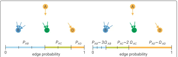
Our approach builds on the generalized hypergeometric ensemble of random graphs (gHypEG) (Casiraghi et al.2016; Casiraghi and Nanumyan2018). This class of models extends the configuration model (CM) (Molloy and Reed1995; 1998) by encoding com-plex topological patterns, while at the same time preserving degree distributions. Block constraints fall into the larger class of patterns that can be encoded by means of gHypEG. For this reason, before introducing the formulation of the block-constrained configura-tion model, we provide a brief overview of gHypEG. More details, together with a more formal presentation, are given in Casiraghi et al. (2016); Casiraghi and Nanumyan (2018). In the configuration model of random graphs, the probability of connecting two ver-tices depends only on their (out- and in-) degrees. In its most common formulation, the configuration model assigns to each vertex as many stubs (or half-edges) as its out-degree, and as many in-stubs as its in-degree. It then proceeds connecting random pairs of vertices joining out- and in-stubs. This is done by sampling uniformly at random one out- and one in-stub from the pool of all out- and in-stubs respectively and then con-necting them, until all stubs are connected. The left side of Fig.1illustrates the case from the perspective of a vertexA. The probability of connecting vertexAwith one of the ver-ticesB,CorDdepends only on the abundance of stubs, and hence on the in-degree of the vertices themselves. The higher the in-degree, the higher the number of in-stubs of the vertex. Hence, the higher the probability to randomly sample a stub belonging to the vertex.

Fig. 1Probabilities of connecting different stubs. Graphical illustration of the probability of connecting two vertices as a function of degrees (left figure), and degree and propensities (right figure)

to an urn problem. Edges are represented by balls in an urn, and sampling from the con-figuration model is described by sampling balls (i.e., edges) from an urn appropriately constructed. For each pair of vertices(i,j), we can denote withkout_i andk_jintheir respec-tive out- and in-degrees. The number of combinations of out-stubs ofiwith in-stubs of

jwhich could be connected to create an edge is then given byk_ioutk_jin. To map this pro-cess to an urn, for each dyad(i,j)we should place exactlyk_ioutk_jinballs of a given colour in the urn (Casiraghi and Nanumyan2018). The process of samplingmedges from the configuration model is hence described by samplingmballs from this urn, and the prob-ability distribution of observing a graphG under the model is given by the multivariate hypergeometric distribution with parameters= {k_ioutkin_j }i,j:

Pr(G|)=

ijij

m

−1

i,j∈V

ij

Aij

, (1)

where Aij denotes the element ij of the adjacency matrix ofG, and the probability of observingGis non-zero only if_ijAij=m.

Generalized hypergeometric ensembles of random graphs further extend this formu-lation. In gHypEG, the probability of connecting two vertices depends not only on the degree (i.e., number of stubs) of the two vertices but also on an independent propensity of the two vertices to be connected, which captures non-degree related effects. Doing so allows constraining the configuration model such that given edges are more likely than others, independently of the degrees of the respective vertices. The right side of Fig.1 illustrates this case, whereAis most likely to connect with vertexD, belonging to the same group, even thoughDhas only one available stub.

In generalized hypergeometric ensembles the distribution over multi-graphs (denoted

G) is formulated such that it depends on two sets of parameters: the combinatorial matrix

As for the case of the configuration model, this process can be seen as sampling edges from an urn. Moreover, specifying a propensity matrix allows to bias the sampling in specified ways, so that some edges are more likely to be sampled than others. The probability distribution over a graphGgivenandis then described by the multivariate Wallenius’ noncentral hypergeometric distribution (Wallenius1963; Chesson1978).

We further denote withAthe adjacency matrix of the multi-graphGand withVits set of vertices, the probability distribution underlying a gHypEGX(,,m)with parameters

,, and withmedges is defined as follows:

Pr(G|,)=

⎡

⎣

i,j∈V

ij

Aij

⎤

⎦ 1

0

i,j∈V

1−z

ij S

Aij

dz (2)

with

S=

i,j∈V

ij(ij−Aij). (3)

In Eq.2, the first term on the right-hand side represents combinatorial effects encod-ing degrees, inherited from the configuration model. The second term, constituted by the integral, encodes the biases that need to be enforced on top of the process defined by the configuration model. Note that, if ij = c for all i,j and for any constant c, i.e., if no biases are enforced on the configuration model, Eq.2 corresponds to Eq. 1 (Casiraghi and Nanumyan2018). The probability distribution for undirected graphs and graphs without self-loops are defined similarly: by excluding the lower triangular entries of the adjacency matrix or by excluding its diagonal entries respectively (we refer to Casiraghi and Nanumyan (2018) for more details).

In the case of large graphs, sampling from an urn without replacement can be approx-imated by sampling with replacement from the same urn. Under this assumption, the approximation allows to estimate the probability given in Eq.2by means of a multinomial distribution with parameterspij=ijij/klklkl.

Block-constrained configuration model

The main modelling assumption that differentiate gHypEGs from SBMs is in the depen-dence/independence of edge probabilities. In particular, while SBMs assume independent edge probabilities, and specifies a Poisson process for the edge generating process, gHy-pEG fixes the total number of edgesm in the model and removes the assumption of independence between edge probabilities. This assumption has the conceptual advan-tage of not assuming an arbitrary edge generating process, such as the Poisson process considered by DC-SBMs.

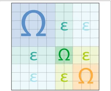
Fig. 2Block-matrix. Structure of a block propensity matrix with 3 different blocks (blue, green, yellow). The entries along the diagonal capture the within-block propensities, those away from the diagonal capture the between-block propensities

However, in the case of a BCCM, the entriesωbibj capture the deviations in terms of edge propensities from the configuration model defined by the matrix, constraining edges into blocks.

The block-matrix Bcan be specified to generate various structures, extending those naturally produced by degrees only, such as a diagonal block-matrix can model graphs with disconnected components. The inclusion of small off-diagonal elements gives rise to standard community structures, with densely connected clusters of vertices. By specifying different types of block-matrices, it is also possible to model core-periphery, hierarchical, or multipartite structures.

The block-constrained configuration modelX(,B,m)withmedges is thus completely defined by the combinatorial matrix, and by the block-matrixBgenerating the propen-sity matrix(B). We can then rewrite the general probability for a gHypEG given in Eq.2 for BCCM:

Pr(G|,B)=

⎡

⎣

i,j∈V

ij

Aij

⎤

⎦ 1

0

i,j∈V

1−z

ω_bibj

S_B Aij

dz (4)

with

SB=

i,j∈V

ωbibj(ij−Aij). (5)

Table 1Comparison of the properties of DC-SBMs and BCCMs

Model DC-SBM BCCM

Multi-edges distribution n2_{independent Poisson n}2_{-variate Wallenius}

Number of edges m preserved in expectation fixed value Distribution of m Poisson(m) fixed value

Degrees preserved in expectation preserved in expectation Distribution of degrees nindependent Poisson n-variate Wallenius

Despite its complicated expression, the probability distribution in Eq.4allows comput-ing probabilities for large graphs, without the need to resort to Monte-Carlo simulations (Fog2008a). This permits the study of large graphs and provides simple model selection methods based on the comparison of likelihoods, such as likelihood-ratio tests, or those based on information criteria. In this article, we will consider model selection based on the comparison of information criteria.

We will adopt the two most commonly used ones: Akaike information criterion (AIC) (Akaike1974), and Schwarz or Bayesian information criterion (BIC) (Schwarz and et al 1978). Both criteria depend on the likelihood function of the models to be compared and penalize for the number of parameters estimated by the model. The model with the lowest score is the preferred one, as it best fits the data without overfitting it. In particular, it is not the absolute size of the score, but it is the difference between values that matters for model selection.

Information-theoretic methods considered here provide a simple way to select the best-approximating model from a candidate set of models. The concept of information criterion has allowed major practical and theoretical advances in model selection and the analysis of complex data sets (Stone1982; Bozdogan1987; DeLeeuw1992). In particular, AIC and BIC allow performing model selection without the need of simulations, nor the assumption of specific asymptotic behaviors of the probability distribution of the model (although BIC assumes thatthe priorsfor the parameters estimated are asymptotically normal). Moreover, the aim of model selection by means AIC and BIC is not to identify exactly the ‘true model,’ i.e., the actual process generating the data, but to propose simpler models that are good approximations of it (Kuha2004). They only allow the selection of the best model among those within a specified set. This means that, if all models in the set are very poor, information criteria will select the best model, but even that relatively best model might be poor in the absolute sense (Burnham and Anderson2004).

The Akaike information criterion for a modelXgiven a graphGis formulated as follows:

AIC(X|G)=2k−2 logLˆ(X|G), (6)

where k is the number of parameters estimated byXand Lˆ(X|G) is the likelihood of model Xgiven the graphG. AIC gives an estimate of the expected, relative Kullback-Leibler distance between the fitted model and the unknown true mechanism generating the observed data. Hence, the best model among a set of models is the one that has the minimal distance from the true process, and thus the one that minimizes AIC.

The Bayesian information criterion for a modelXgiven a graphGis given by:

BIC(X|G)=log(m)k−2 log

ˆ

wherekis the number of parameters estimated byX,mis the number of observations, i.e., edges, andL(Xˆ |G)is the likelihood of modelXgiven the graphG. Similarly to AIC, the best model in a set according to BIC is the one which minimizes the criterion. Because of the presence of a higher penalty for model size, BIC tends to select models with lower parameters compared to AIC.

As mentioned above, what matters for model selection is the difference between the value of AICs or BICs and not their absolute values. For this reason, it is helpful to rank models in terms of their differences from the model which minimizes a given criterion. Suppose that there areRmodels, and we want to find the best one according to either AIC or BIC. Let AICminbe the model which minimizes AIC for a given dataset. Then we

can define the AIC differencesAIC_i as the difference AICi−AICminof the AIC score for

modeli ∈ {1,. . .,R}, and the model which minimizes AIC. BIC differences are defined in a similar manner. While AIC and BIC differences are useful in ranking models, it is possible to quantify the plausibility of each model by defining relative likelihoods for the models. Specifically, the quantitye−1/2idefines the relative likelihood of modeligiven the data (Burnham and Anderson2004). To better interpret relative likelihoods, statisti-cians usually normalize relative likelihoods to be a set of positive weightswidefined as

wi:=

e−1/2i

_R

r=1e−1/2r

. (8)

In the case of AIC, such model weights are usually referred to as Akaike weights and are considered to be the weight of evidence in favor of modelibeing the best model. In the case of BIC, instead, the weights define the posterior model probabilities. The biggeri is, the smallerwiand the less plausible is modelias being the actual best model based on the design and sample size used. These weights provide an effective way to scale and interpret theivalues and hence select the best model (Burnham and Anderson2004).

In the next sections, we describe how BCCM can be used to generate graphs and how to fit its parameters to an observed graph. Because the absolute values of AIC and BIC are not important, and only relativeis matter, in the following we will usually report only the value of the relative differences.

Generating realizations from the BCCM. BCCM is a practical generative model that allows the creation of synthetic graphs with complex structures by drawing realizations from the multivariate Wallenius non-central hypergeometric distribution. The process of generating synthetic graphs can be divided into two tasks. First, it is needed to specify the degree sequences for the vertices. It can be accomplished by, e.g., sampling the degree sequences from a power-law or exponential distributions. From the degree sequences we can generate the combinatorial matrix, specifying its elementsij = kioutkjin, where

k_ioutis the out-degree of vertexi. Second, we need to define a block-matrixB, whose ele-ments specify the propensities of observing edges between vertices, between and within the different blocks.

The block-matrixBtakes the form given in Eq.9:

B=

⎡ ⎢ ⎢ ⎣

ω1 . . . ω1B .. .

ωB1 . . . ωB

⎤ ⎥ ⎥

Elementsωkl, withk,l ∈ {1,. . .,B}, should be specified such that the ratio between any two elements corresponds to the chosen odds-ratios of observing an edge in the block corresponding to the first element instead of the block corresponding to the second ele-ment, given the degrees of the corresponding vertices were the same. For example,ω1/ω32

corresponds to the odds-ratio of observing an edge between vertices in block 1 compared to an edge between block 2 and block 3. Note that in the case of an undirected graph,

ωkl = ωlk ∀k,l ∈ {1,. . .,B}. On the other hand, in the case of a directed graph, blocks may have a preferred directionality, i.e., edges between blocks may be more likely in one direction. In this case, we may chooseωkl=ωlk.

Once the parameters of the model are defined, we sample graphs withmedges from the BCCMX(,B,m)defined by the combinatorial matrix, and the block-propensity matrixB defined by B. As described in the previous section, sampling a graph from

X(,B,m)corresponds to samplemedges according to the multivariate Wallenius non-central hypergeometric distribution.

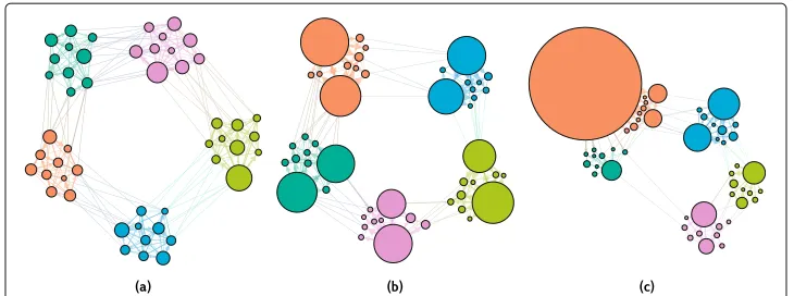
Examples We can specify different types of clustered graphs using this construction. As a demonstrative example, we define a block-matrix with five blocks connected in a ring. Each block is as dense as the others, and blocks are weakly connected with only their closest neighbors. The block-matrix quantifying these specification is given as

B=

⎡ ⎢ ⎢ ⎢ ⎢ ⎢ ⎢ ⎣

1 0.1 0 0 0 0 1 0.1 0 0 0 0 1 0.1 0 0 0 0 1 0.1 0.1 0 0 0 1

⎤ ⎥ ⎥ ⎥ ⎥ ⎥ ⎥ ⎦

. (10)

According to the choice made in Eq.10, edges within diagonal blocks are 10 times more likely than edges within off-diagonal blocks.

After fixing this block-matrix, we can define different degree sequences for the ver-tices. We highlight here the results obtained when fixing three different options in a directed graph without self-loops, withn= 50 vertices andm= 500 edges. We gener-ate realizations by specifying the combinatorial matrixand the block propensity matrix and exploiting the random number generator provided by Fog (2008b) in theRlibrary BiasedUrn.

Fig. 3 Realisations from a block-constrained configuration model obtained by fixing the block-matrixBand varying the out-degree distribution. Each realisation is obtained from a BCCM withN=50 vertices and m=500 directed edges. The vertices are separated into 5 equally sized blocks and the block-matrixBis given by Eq.10. On left side,ais a realisation from a BCCM where the degree distributions are uniform. It corresponds to a realisation from a standard SBM. In the center,bis a realisation obtained by drawing the out-degree distribution of the vertices in each block from a power-law distribution with parameterα=1.8. On the right side,cis a realisation obtained by drawing the out-degree distribution of all vertices from the same power-law. All graphs are visualised using the force-atlas2 layout with weighted edges. Out-degrees determine vertex sizes, and edge widths the edge counts

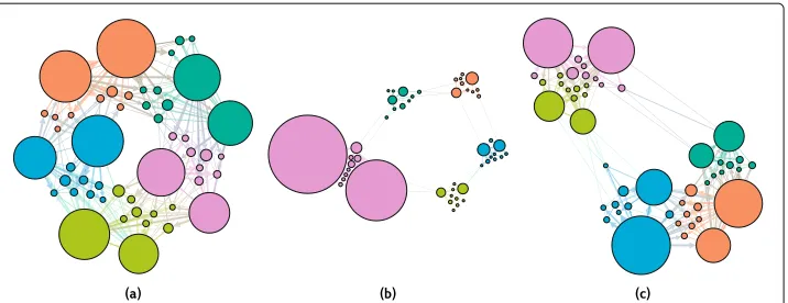
Instead of varying the degree sequences of the underlying configuration model, we can as well alter the strength of the block structure, changing the block-matrixB. Similarly to what we did above, we show three different combinations of parameters. First, we set the within group parametersω_biequal to the between group parametersω_bibj ∀i,j. Second, we set the parametersωb1 = 10 so that the more edges are concentrated in the first block. Third, we set the parameter to reconstruct a hierarchical structure. We modify the parametersωb1b2 =ωb3b4 =ωb4b5 =0.8 to model graphs with two macro clusters weakly connected, where the one is split into two clusters strongly connected and the other into three clusters strongly connected. Realizations drawn from each of these three models are shown in Fig.4.

Fitting the block-matrix. In DC-SBMs the number of edges between each pair(i,j)of vertices are assumed to be drawn from independent Poisson distributions, with parame-tersθiθjωbibj. LetAbαbβ =

i∈bα,j∈bβAijdenote the number of edges between all vertices

ithat are in the blockbαandjin blockbβ. We further denotebithe partition of vertex

i. Exploiting the independence of probabilities, the maximum likelihood estimatesθiand

ωbibj of the parametersθiandωbibjare given byθi:=ki/κbiandωbibj :=Abibj(Karrer and Newman2011).

Fig. 4Realisations from a block-constrained configuration model obtained by fixing the out-degree distribution and varying the parameters within the block-matrixB. Each realisation is obtained from a BCCM withN=50 vertices andm=500 directed edges. The out-degree distribution of the vertices in each block follows a power-law distribution with parameterα=1.8 The vertices are separated into 5 equally sized blocks and the structure of the block-matrixBis given by Eq.10, but in each graph the values of some of the parametersωbibjare changed. On left side,ais a realisation from a BCCM where the between-block

parameters are increased to 1. In the center,bis a realisation obtained by increasing the parameterωb1that controls for the internal cohesion of the first block. On the right side,cis a realisation obtained by increasing to 0.8 the between-block parametersωb1b2,ωb3b4, andωb4b5, to create a hierarchical block structure where the first two blocks are part of a macro cluster, and the last three blocks are part of another. All graphs are visualised using the force-atlas2 layout with weighted edges. Out-degrees determine vertex sizes, and edge widths the edge counts

In gHypE, the entries of the expected adjacency matrixAijare obtained by solving the following system of equations (Casiraghi and Nanumyan2018):

1− A11

11

1

11 =

1−A12

12

1

12

=. . . (11)

with the constraint_i,j∈VAij =m.

Because to estimate BCCM we need to fix the expectation of the number of edges between blocks and not between dyads, we proceed as described below. We denote with

bα =

i,j∈bαij the sum of all the elements of the matrixcorresponding to those

dyads. Then, we fix the expectations of the ensemble such that the number of edges between and within blocks is given byAbαs. Hence, in the case of the block-constrained

configuration model withBblocks we estimate theB·(B+1)/2 parametersωbαbβs

con-stituting the block-matrixBˆ solving the following set of independent equations, defined up to an arbitrary constantk:

⎧ ⎪ ⎪ ⎪ ⎪ ⎨ ⎪ ⎪ ⎪ ⎪ ⎩

1− Ab1 b₁

1

ω_b

1 =_k .. .

1−AbB bB

1

ω_bB

=k.

(12)

Solving for ωbαbβ, we find that the entries of the block-matrix Bˆ that preserve in

expectation the observed number of edges between and within blocks are given by

ωbαbβ := −log

1− Abαbβ

bαbβ

. (13)

When the parameters of the BCCM are estimated as described here, the block-constrained configuration model has the advantageous property of asymptotic consis-tency. It means that, if the method described here is applied to synthetic graphs generated from a BCCM, the technique introduced in this article can correctly recover the original model.

Estimating thematrix. In the case of the configuration model defined by Eq.1, the elementsij of the combinatorial matrix are defined askini kjout. This definition gener-ates a model that preserves the degree sequences of the observed graph (Casiraghi and Nanumyan2018). By generalizing the model according to Eq. 4, where the propensity matrix is estimated as in Eq.13, we introduce constraints on the edge sampling process that allows preserving the observed number of edges in each block. The estimated param-eters can hence be interpreted as the bias needed to modify the configuration model to reproduce block structures.

To preserve the degrees of the observed graph in the BCCM, we need to update the combinatorial matrix such that it defines the degree-sequences of the corresponding con-figuration model like there were no block constraints. We achieve this by redefining the combinatorial matrix elements asij=kini kjoutθiinθjout. The estimation ofandis then performed by an expectation-maximization algorithm that iteratively estimatesand such that degrees and blocks are preserved in expectation. A pseudo-code for the algo-rithm estimating the parameters of a BCCM model for directed graphs is provided in Algorithm 1. In the case of undirected graphs, the algorithm is adapted according to the fact thatandare upper-triangular matrices.

Algorithm 1estimateBCCM(G, tolerance):Adjust entries ofto match expected degrees (based on,) to observed degrees (based onG), within ‘tolerance’ error, where the error is computed as the mean absolute error (MAE).

Require: Gobserved graph, tolerance Ensure: ,

1: k_vout←_xAv,x{out-degrees}

2: kin

v←

xAx,v{in-degrees}

3: m←_vk_vout{number of edges}

4: vw←kvout·kinw {initializefor allv,w∈G}

5: Abαbβ←

x∈bα,y∈bβAx,y{number of edges in blockbαβ}

6: b_αb_β←x∈bα,y∈bβx,y{combinatorial matrix for blockbαβ}

7: ωb_αb_β:= −log(1− Ab_αb_β

b_αb_β){initializefor allv,w∈G}

8: repeat

9: kin

v←

xE(Ax,v){Expectation for in-degrees}

10: vw←vw·k

in w kin

w {Correction for in-degrees}

11: kout

v ←

xE(Av,x){Expectation for out-degrees}

12: vw←vw·k

out v

kvout {Correction for out-degrees}

13: bαbβ←

x∈b_α,y∈b_βx,y{new combinatorial matrix for blockbαβ}

14: ωbvbw := −log(1− A_bvbw

bvbw){ML estimation ofωbvbwfor allv,w}

15: untilMAE(kout,kout)+MAE(kin,kin)≤tolerance

Case studies

We conclude the article with a case study analysis of synthetic and empirical graphs. We highlight the interpretability of the resulting block-constrained configuration models in terms of deviations from the classical configuration model. In particular, a weak com-munity structure in a graph is reflected in a small contribution to the likelihood of the estimated block-matrix. On the other hand, a strong community structure is reflected in a substantial contribution to the likelihood of the estimated block-matrix. Here, we quan-tify this difference employing AIC or BIC. However, other information criteria may also be used. Moreover, studying the relative values of the estimated parameters in the block matrices quantifies how much the configuration model has to be biased towards a block structure to fit the observed graph optimally. The more different are the values of the parameters, the stronger is the block structure compared to what is expected from the configuration model.

We start by analyzing synthetic graphs generated according to different rules, and we show that fitting the block-constrained configuration model parameters allows selecting the correct, i.e., planted, partition of vertices, among a given set of different partitions. We perform three experiments with large directed graphs with clusters of different sizes. Finally, we conclude by employing the BCCM to compare how well different partitions obtained by different clustering algorithms fit popular real-world networks.

Analysis of synthetic graphs. We generate synthetic graphs incorporating ‘activities’ of vertices in a classical SBM, to be able to plant different out-degree sequences in the syn-thetic graphs. First, we need to assign the given activity to each vertex. Higher activity means that the vertex is more likely to have a higher degree. Second, we need to assign vertices to blocks and assign a probability of sampling edges to each block. Densely con-nected blocks have a higher probability than weakly concon-nected blocks. The graph is then generated by a weighted sampling of edges with replacement from the list containing all dyads of the graph. The product between the activity corresponding to the from-vertex and the weight corresponding to the block to which the dyad belongs gives sampling-weights for each dyad. The probabilities of sampling edges correspond to the normalized weights so that their sum is 1.

For example, let us assume we want to generate a 3-vertices graph with two clusters. We can fix the block weights as follows: edges in block 1 or 2 have weightw1 andw2

respectively; edges between block 1 and block 2 have weightw12. Table2shows the list

of dyads from which to sample together with their weights, where the activity of vertices is fixed to(a1,a2,a3), and the first two vertices belong to the first block. Note that if the

activities of the vertices were all set to the same value, this process would correspond to the original SBM. In the following experiments, we generate different directed graphs withN = 500 vertices,m = 40000 edges, and different planted block structures and vertex activities.

Table 2Edge list with weights for the generation of synthetic graphs with given vertex activities and block structure

dyad activity block id block weight sampling weight

1 – 1 a1 1 w1 a1w1

1 – 2 a1 1 w1 a1w1

1 – 3 a1 12 w12 a1w12

2 – 1 a2 1 w1 a2w1

2 – 2 a2 1 w1 a2w1

2 – 3 a2 12 w12 a2w12

3 – 1 a3 12 w12 a3w12

3 – 2 a3 12 w12 a3w12

3 – 3 a3 2 w2 a3w2

on. In the first experiment, we do not assign block weights so that the graphs obtained do not show any consistent cluster structure, and have a skewed out-degree distribution according to the fixed vertex activity (correlation∼1).

First, we assign the vertices randomly to two blocks. We proceed by estimating the parameters for an SBM and a BCCM, according to the blocks to which the vertex has been assigned. Since no block structure has been enforced and the vertex has been assigned randomly to blocks, we expect that the estimated parameters for the block matricesBˆSBM

andBˆBCCM will all be close to 1 (when normalized by the maximum value), reflecting

the absence of a block structure. The resulting estimated parameters for an exemplary realisation are reported in Eq.14.

ˆ BSBM=

1.0000000 0.9992577 0.9992577 0.9603127

ˆ

BBCCM=

0.9808935 1.0000000 1.0000000 0.9805065

(14)

As expected, the estimated values for both models are close to 1.

After changing the way vertices are assigned to blocks, we repeat the estimation of the two models. Now, we separate the vertices into two blocks such that the first 250 vertices ordered by activity are assigned to the first block and the last 250 to the second one. We expect that the SBM will assign different parameters to the different blocks because now the first block contains all vertices with high degree, and the second block all vertices with low degree. Hence, most of the edges are found between vertices in the first block or between the two blocks. Differently, from the SBM, the BCCM corrects for the observed degrees. Hence, we expect that the parameters found for the block-matrix will be all close to 1 again, as no structure beyond that one generated by degrees is present. Thus the block assignment does not matter for the estimated parameter. The block matrices for the two models, estimated for the same realisation used above, are provided in Eq.15.

ˆ BSBM=

1.000000 0.597866 0.597866 0.194896

ˆ

BBCCM=

0.997024 0.995108 0.995108 1.000000

(15)

We observe that the SBM assigns different values to each block, impairing the inter-pretability of the result. In particular, the parameters ofBˆSBM show the presence of a

core-periphery structure which cannot be distinguished from what obtained naturally from skewed degree distributions. The estimation of BˆBCCM, on the contrary,

In the second synthetic experiment, we highlight the model selection features of the BCCM. Thanks to the fact that we are able to compute the likelihood of the model directly, we can efficiently compute information criteria such as AIC or BIC to perform model selection. We generate directed graphs with self-loops withN=500 vertices,m=40000 edges, and two equally sized clusters. Again, we generate vertex activities from an expo-nential distribution with rateλ= N/m. We fix the block weights to bew1= 1,w2 =3,

andw12 =0.1. Using this setup, we can generate synthetic graphs with two clusters, one

of which is denser than the other. If we fit a BCCM to the synthetic graph with the cor-rect assignment of vertices to blocks, we obtain the following block-matrixBˆBCCMfor an

exemplary realization:

ˆ

BBCCM=

1.1760878 0.1108463 0.1108463 3.0000000

(16)

We note that we approximately recover the original block weights used to generate the graph.

We can now compare the AIC obtained for the fitted BCCM model, AICBCCM =

662060, to that obtained from a simple configuration model (CM) with no block assign-ment, AICCM = 693540. The CM model is formulated in terms of a gHypEG where the

propensity matrix ≡ 1. The AIC for the BCCM is considerably smaller, confirming that the model with block structure fits better the observed graph. In terms of AIC differ-ences,AIC_BCCM = 0 andAIC_CM = 31480. This corresponds to model weightswBCCM ∼ 1

andwCM ∼0. That means that there is no evidence for model CM. As a benchmark, we

compute the AIC for BCCM models where the vertices have been assigned randomly to the two blocks.

Table3reports the AIC differences obtained for 1000 random assignment of vertices to the blocks, computed on the same observed graph. We observe that this usually results in values close to that of the simple configuration model, as the block assignments do not reflect the structure of the graph. In a few cases, a small number of vertices are correctly assigned to blocks, showing a slight reduction in AIC, which is however far from that of the correct assignment.

BCCM also allows comparing models with a different number of blocks. To do so, we separate the vertices in one of the blocks of the model above into two new blocks. Because we add more degrees of freedom, we expect an increase in the likelihood of the new BCCM with three blocks, but this should not be enough to give a considerable decrease in AIC. Since the synthetic graph has been built planting two blocks, the AIC should allow us to select as an optimal model the BCCM with two blocks. The resulting block-matrix

ˆ

B(_BCCM3) with three blocks is reported in Eq.17.

ˆ

B(_BCCM3) =

⎡ ⎢ ⎣

1.1739475 1.1797875 0.1088987 1.1797875 1.1706410 0.1129094 0.1088987 0.1129094 3.0000000

⎤ ⎥

⎦ (17)

Table 3AIC_i values from the model with the correct assignment vertices-blocks, obtained for 1000 random assignment of vertices to the blocks, computed on the same observed graph

Min. 1st Qu. Median Mean 3rd Qu. Max.

AIC

We see that the estimated model fits different parameter values for the two sub-blocks, since the added parameters can now accommodate for random variations generated by the edge sampling process. However, as expected, there is no (statistical) evidence to sup-port the more complex model. In fact, comparing the AIC values we obtain AIC(_BCCM3) = 662065 >662060 = AICBCCM. This corresponds toAIC_BCCM = 0 andAIC_BCCM(3) = 5. In

terms of model weights, we getwBCCM∼0.92 andw(_BCCM3) ∼0.08. That means that there

is strong evidence against the more complex model, as the probability that the more com-plex model is closer to the real process is only 0.08, given the data used to estimate the model.

To provide more evidence in support of this selection procedure, we can repeat this experiment on 100 samples from the same model used before. The results provide median AIC differences ofBCCM = 0 and(_BCCM3) = 4.32. Moreover, out of the 100 samples

only 7 have AIC(_BCCM3) < AICBCCM. This is aligned with the probability of 0.08

esti-mated employing model weights. We can thus successfully use BCCM to perform model selection, both when a different number of clusters or various vertex assignments are used.

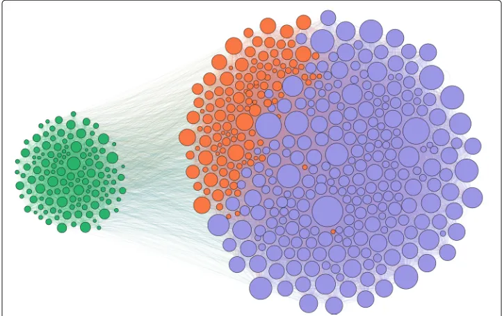
In the third experiment, instead of two clusters, we plant three clusters of different sizes

(|B1| = 250,|B2| = 125,|B3| = 125). We choose the block parameters such that one

of the smaller clusters is more densely connected with the bigger cluster, and the smaller cluster is relatively denser than the others. To do so we choose the block weights as fol-lows:w1 = w2 = 1,w3 = 3,w13 = w23 = 0.1,w12 = 0.8. As before, we draw vertex

activities from an exponential distribution with parameterλ=N/m. One exemplary real-isation is plotted in Fig.5. The plot clearly shows the separation into three clusters, with

cluster 1 (purple) and 2 (orange) more densely connected to each other than to cluster 3 (green). Fitting the same BCCM as before allows comparing the AICs for the three-blocks BCCM to the 2-block BCCM. In this case, we expect that the model with three blocks will fit considerably better the graph. Results of the fitting for the realisation plotted in Fig.5give AIC(_BCCM3) =673585<699765=AIC(_BCCM2) , correctly selecting the more com-plex model. This corresponds toAIC

BCCM(2) =26180 andAIC_BCCM(3) =0. In terms of model

weights, we getw(_BCCM2) ∼ 0 andw(_BCCM3) ∼ 1. That means that there is strong evidence against the simpler model.

It is known that AIC does not punish model complexity as much as BIC. For this reason, in this case, we also compare the values of BIC obtained for the two models. Also in this case, with BIC(_BCCM3) =2822787<2848941=BIC(_BCCM2) , the information criterion allows to correctly select the model with 3 blocks. Comparing posterior probabilities for the two models, we get againw(_BCCM2) ∼0 andw(_BCCM3) ∼1.

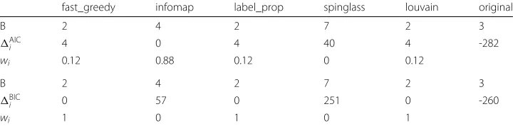
Finally, we can use AIC and BIC to evaluate and rank the goodness-of-fit different block assignments that are obtained from various community detection algorithms. This allows choosing the best block assignment in terms of deviations from the configuration model, i.e., which of the detected block assignment better captures the block structure that goes beyond that generated by the degree sequence of the observed graph. We compare the result obtained from 5 different algorithms run using theirigraphimplementation for R. In the following we use:cluster_fast_greedy, a greedy optimisation of modular-ity (Clauset et al.2004);cluster_infomap, the implementation ofinfomapavailable throughigraph(Rosvall and Bergstrom2008);cluster_label_prop, label prop-agation algorithm (Raghavan et al.2007);cluster_spinglass, find communities in graphs via a spin-glass model and simulated annealing (Reichardt and Bornholdt2006); cluster_louvain, the Louvain multi-level modularity optimisation algorithm (Blon-del et al.2008). As the modularity maximization algorithms are implemented only for undirected graphs, we apply them to the undirected version of the observed graph. The results of the application of the 5 different algorithms on the realisation shown in Fig.5 are reported in the table in Table4.

The five different community detection algorithms find three different block structures. Three of them are not able to detect the third block, while the other two algorithms split the vertices into too many blocks. AIC ranks bestinfomapeven though it detects one block too many. BIC punishes for the number of parameters more, so ranks best

Table 4Comparison of the goodness-of-fit of 5 different block structures detected by five different community detection algorithms

fast_greedy infomap label_prop spinglass louvain original

B 2 4 2 7 2 3

AIC

i 4 0 4 40 4 -282

wi 0.12 0.88 0.12 0 0.12

B 2 4 2 7 2 3

BIC

i 0 57 0 251 0 -260

wi 1 0 1 0 1

the 2-blocks. These results are consistent when repeating the experiment with differ-ent synthetic graphs generated from the same model. It is worth noting that none of the community detection algorithms was able to detect the planted block structure correctly. However, both the AIC and BIC of the BCCM fitted with the correct block structure are lower than those found by the different algorithms. This shows that information cri-teria computed using BCCM have the potential to develop novel community detection algorithms that are particularly suited for applications where degree correction is crucial. However, the development of such algorithms is beyond the scope of this article and is left to future investigations.

Analysis of empirical graphs We conclude this article by providing a comparison of the BCCM obtained by fitting the block structures detected by the five community detection algorithms described above on five different real-world networks. The results show that different algorithm performs better for different graphs, highlighting the non-trivial effect that degrees have on block structure and community detection in general.

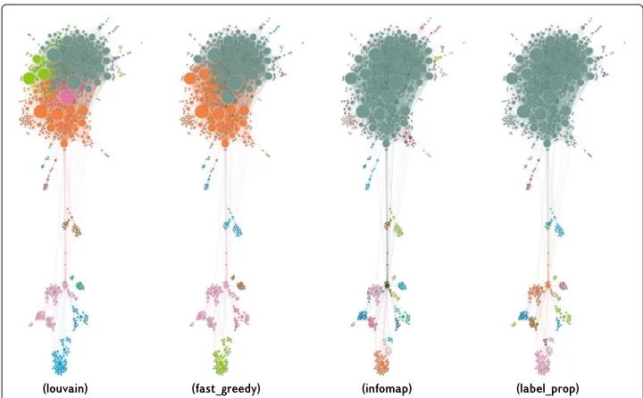
We study five well-known graphs with heterogeneous characteristics and sizes. All graphs are multi-edge, and are freely available as dataset within theigraphdata R pack-age. The first graph analyzed isrfid: hospital encounter network data. It consists of 32424 undirected edges between 75 individuals (Vanhems et al.2013). The second graph analyzed iskarate: Zachary’s Karate Club. It consists of 231 undirected edges between 34 vertices (Zachary1977). The third graph analyzed isUKfaculty: Friendship network of a UK university faculty. It consists of 3730 directed edges between 81 vertices (Nepusz et al.2008). The fourth graph isUSairports: US airport network of December 2010. It consists of 23473 directed edges between 755 airports (Von Mering et al.2002). It has self-loops. The graph is plotted in Fig.6, using the force-atlas2 layout (Jacomy et al.2014). The four different plots are colored according to the block structures detected by four of the five algorithms (cluster_spinglasscannot be applied as the graph is discon-nected). They are ordered by increasing AIC. From the visualization, we can see that the best block structure is the one who can separate three different blocks within the largest cluster of vertices (top of the visualizations). In particular, it is essential to note that the largest cluster consists of high- and low-degree vertices. If these vertices are belonging to the same block, the configuration model predicts then high-degree vertices should be connected by many edges (similarly to the first synthetic experiment described above). However, we observe then some of these high-degree vertices are separated and mainly connected to low-degree vertices. For this reason, block structures that can separate these high-degree vertices into different blocks rank higher than others. The fifth graph ana-lyzed isenron: Enron Email Network. It consists of 125409 directed edges between 184 individuals (Priebe et al.2005). It has self-loops.

Fig. 6USairports graph visualisation.USairportsgraph visualisation. The graph is plotted by means of the force-atlas2 layout with weighted edges, and the size of the vertices reflects their out-degrees. Only the largest connected component of the graph is shown. The visualisations clearly show the block structure that characterises this graph. The vertices in the four visualisations are coloured according to the labels detected applying four community detection algorithms, as described in Table5. The visualisations are ordered from left to right according to the AIC of the BCCM fitted to observed graph according to the corresponding block structure. From left to right, we see the colours corresponding to the labels obtained from louvain,

fast_greedy, infomap and label_propagation detection algorithms respectively. We highlight the fact that the ranking according to AIC corresponds approximately to the ability of the algorithms to detect the separation between high-degree (and low-degree) vertices within the largest cluster, at the top of the visualisations. The reason for this is that within the largest cluster there are clear deviations from what the configuration model predicts, i.e., high-degree vertices tend to connect to each other, and the best BCCMs captures more of these deviations

of blocks. The algorithm that provides the largest number of blocks is highlighted in italic.

Conclusion

Table 5Results of the fitting of BCCM to five real-world graphs, with vertex blocks given obtained from five different community detection algorithms

Data specifications

dataset vertices edges directed self-loops

rfid 75 32424 False False

karate 34 231 False False

UKfaculty 81 3730 True False

USairports 755 23473 True True

enron 184 125409 True True

Number of clusters

dataset fast_greedy infomap label_prop spinglass louvain

rfid 6 4 3 7 6

karate 3 3 3 4 4

UKfaculty 5 10 7 7 5

USairports 28 57 40 NA 21

enron 11 22 20 NA 10

AIC

i

dataset fast_greedy infomap label_prop spinglass louvain

rfid 1856 12370 13523 0 1856

karate 28 28 28 4 0

UKfaculty 992 0 960 523 992

USairports 1903 2759 5133 NA 0

enron 0 9881 46945 NA 1956

BIC

i

dataset fast_greedy infomap label_prop spinglass louvain

rfid 1798 12219 13339 0 1798

karate 14 14 14 4 0

UKfaculty 743 0 792 355 743

USairports 3315 14227 9883 NA 0

enron 0 11702 48347 NA 1849

The first table reports information about the five different graphs used. The second table reports the number of clusters detected by each algorithm for each dataset. The algorithm detecting the smallest number of clusters is highlighted in bold, and the algorithm detecting the largest number of clusters is highlighted in italic. The third table reports AIC differences of the different models computed using the different vertex blocks. The fourth table reports BIC differences of the different models computed using the different vertex blocks. The best model, i.e., the one with the lowest AIC/BIC score, respectively, is highlighted in bold. Because the spin-glass algorithm is not suitable for disconnected graphs, no result is reported for this method for the last two real-world graphs

framework, provides a natural method to quantify the optimal number of blocks needed to model given real-world graph. The statistical significance of a block structure can be studied performing likelihood-ratio tests (Casiraghi et al.2016), or comparing infor-mation criteria such as AIC, BIC, or the description length of the estimated models. Furthermore, within the framework of generalized hypergeometric ensembles block-constrained configuration models can be extended, including heterogeneous properties of vertices or edges (see Casiraghi (2017)).

community detection algorithms suitable for applications where degree correction is par-ticularly valuable, and where the assumption of an arbitrary edge generating process is not acceptable.

Abbreviations

AIC: Akaike information criterion; BCCM: Block-constrained configuration model; BIC: Bayesian information criterion; DC-SBM: Degree-corrected stochastic block model; gHypEG: Generalised hypergeometric ensemble of random graphs; SBM: Stochastic block model

Acknowledgements

The author thanks Frank Schweitzer for his support and valuable comments, and Laurence Brandenberger, Giacomo Vaccario and Vahan Nanumyan for useful discussions.

Authors’ contributions

The author read and approved the final manuscript.

Funding Not applicable.

Availability of data and materials

The datasets generated and/or analysed during the current study are available as agitHubrepository,https://github. com/gi0na/BCCM--Supporting-Material.git. The combinatorial matrices corresponding to Fig.3b and c are included within the article (and its additional file(s)). A software implementation of the BCCM can be found as part of theR packageghypernetavailable athttps://github.com/gi0na/ghypernet.git.

Competing interests

The authors declare that they have no competing interests.

Received: 23 July 2019 Accepted: 28 November 2019

References

Akaike H (1974) A new look at the statistical model identification. IEEE Trans Autom Control 19(6):716–723.https://doi. org/10.1109/TAC.1974.1100705

Bender EA, Canfield ER (1978) The asymptotic number of labeled graphs with given degree sequences. J Comb Theory Ser A 24(3):296–307.https://doi.org/10.1016/0097-3165(78)90059-6

Blondel VD, Guillaume J-L, Lambiotte R, Lefebvre E (2008) Fast unfolding of communities in large networks. J Stat Mech Theory Exp 2008(10):10008

Bozdogan H (1987) Model selection and Akaike’s Information Criterion (AIC): The general theory and its analytical extensions. Psychometrika 52(3):345–370.https://doi.org/10.1007/BF02294361

(2004) Model Selection and Multimodel Inference(Burnham KP, Anderson DR, eds.). Springer, New York.https://doi.org/ 10.1007/b97636.http://link.springer.com/10.1007/b97636

Caldarelli G, Chessa A, Pammolli F, Gabrielli A, Puliga M (2013) Reconstructing a credit network. Nat Phys.https://doi.org/ 10.1038/nphys2580

Casiraghi G (2017) Multiplex Network Regression: How do relations drive interactions? arXiv preprint arXiv:1702.02048. 1702.02048

Casiraghi G, Nanumyan V (2018) Generalised hypergeometric ensembles of random graphs: the configuration model as an urn problem.1810.06495

Casiraghi G, Nanumyan V, Scholtes I, Schweitzer F (2016) Generalized Hypergeometric Ensembles: Statistical Hypothesis Testing in Complex Networks. arXiv preprint arXiv:1607.02441.1607.02441

Chesson J (1978) Measuring Preference in Selective Predation. Ecology 59(2):211–215

Chung F, Lu L (2002) Connected Components in Random Graphs with Given Expected Degree Sequences. Ann Comb 6(2):125–145.https://doi.org/10.1007/PL00012580

Chung F, Lu L (2002) The average distances in random graphs with given expected degrees. Proc Natl Acad Sci 99(25):15879–15882.https://doi.org/10.1073/pnas.252631999

Clauset A, Newman ME, Moore C (2004) Finding community structure in very large networks. Phys Rev E 70(6):066111 Consul PC, Jain GC (1973) A Generalization of the Poisson Distribution. Technometrics 15(4):791–799.https://doi.org/10.

1080/00401706.1973.10489112

DeLeeuw J (1992) Introduction to Akaike 1973 Information Theory and an Extension of the Maximum Likelihood Principle:599–609.https://doi.org/10.1007/978-1-4612-0919-5_37. http://link.springer.com/10.1007/978-1-4612-0919-5_37

Erdös P, Rényi A (1959) On random graphs I. Publ Math Debrecen 6:290–297

Fienberg SE, Meyer MM, Wasserman SS (1985) Statistical Analysis of Multiple Sociometric Relations. J Am Stat Assoc 80(389):51–67.https://doi.org/10.1080/01621459.1985.10477129

Fog A (2008) Calculation Methods for Wallenius’ Noncentral Hypergeometric Distribution. Commun Stat Sim Comput 37(2):258–273.https://doi.org/10.1080/03610910701790269

Fog A (2008) Sampling Methods for Wallenius’ and Fisher’s Noncentral Hypergeometric Distributions. Commun Stat Sim Comput 37(2):241–257.https://doi.org/10.1080/03610910701790236

Holland PW, Laskey KB, Leinhardt S (1983) Stochastic blockmodels: First steps. Social Networks 5(2):109–137.https://doi. org/10.1016/0378-8733(83)90021-7

Jacomy M, Venturini T, Heymann S, Bastian M (2014) Forceatlas2, a continuous graph layout algorithm for handy network visualization designed for the gephi software. PLoS ONE 9(6):98679

Karrer B, Newman MEJ (2011) Stochastic blockmodels and community structure in networks. Phys Rev E 83(1):16107. https://doi.org/10.1103/PhysRevE.83.016107

Krivitsky PN (2012) Exponential-family random graph models for valued networks. Electron J Stat 6:1100–1128.https:// doi.org/10.1214/12-EJS696

Kuha J (2004) AIC and BIC. Soc Methods Res 33(2):188–229.https://doi.org/10.1177/0049124103262065

Melnik S, Porter MA, Mucha PJ, Gleeson JP (2014) Dynamics on modular networks with heterogeneous correlations. Chaos Interdiscip J Nonlinear Sci 24(2):023106

Molloy M, Reed B (1995) A critical point for random graphs with a given degree sequence. Random Struct Algoritms 6(2-3):161–180.https://doi.org/10.1002/rsa.3240060204

Molloy M, Reed B (1998) The Size of the Giant Component of a Random Graph with a Given Degree Sequence. Comb Probab Comput 7(3):295–305

Nanumyan V, Garas A, Schweitzer F (2015) The Network of Counterparty Risk: Analysing Correlations in OTC Derivatives. PLoS ONE 10(9):0136638.https://doi.org/10.1371/journal.pone.0136638.1506.04663

Nepusz T, Petróczi A, Négyessy L, Bazsó F (2008) Fuzzy communities and the concept of bridgeness in complex networks. Phys Rev E 77(1):016107

Newcomb T, Heider F (1958) The Psychology of Interpersonal Relations. Am Soc Rev.https://doi.org/10.2307/2089062. arXiv:1011.1669v3

Newman MEJ, Peixoto TP (2015) Generalized Communities in Networks. Phys Rev Lett 115(8):088701.https://doi.org/10. 1103/PhysRevLett.115.088701

Newman MEJ, Reinert G (2016) Estimating the Number of Communities in a Network. Phys Rev Lett 117(7):078301. https://doi.org/10.1103/PhysRevLett.117.078301

Park J, Newman MEJ (2004) Statistical mechanics of networks. Phys Rev E 70(6):066117.https://doi.org/10.1103/PhysRevE. 70.066117

Peixoto TP (2012) Entropy of stochastic blockmodel ensembles. Phys Rev E 85(5):056122.https://doi.org/10.1103/ PhysRevE.85.056122

Peixoto TP (2014) Hierarchical Block Structures and High-Resolution Model Selection in Large Networks. Phys Rev X 4(1):011047.https://doi.org/10.1103/PhysRevX.4.011047

Peixoto TP (2015) Model Selection and Hypothesis Testing for Large-Scale Network Models with Overlapping Groups. Phys Rev X 5(1):011033.https://doi.org/10.1103/PhysRevX.5.011033

Peixoto, TP (2017) Nonparametric Bayesian inference of the microcanonical stochastic block model. Phys Rev E 95(1):012317.https://doi.org/10.1103/PhysRevE.95.012317

Peixoto TP (2018) Reconstructing Networks with Unknown and Heterogeneous Errors. Phys Rev X 8(4):041011.https:// doi.org/10.1103/PhysRevX.8.041011

Priebe CE, Conroy JM, Marchette DJ, Park Y (2005) Scan statistics on enron graphs. Comput Math Org Theory 11(3):229–247 Raghavan UN, Albert R, Kumara S (2007) Near linear time algorithm to detect community structures in large-scale

networks. Phys Rev E 76(3):036106

Reichardt J, Bornholdt S (2006) Statistical mechanics of community detection. Phys Rev E 74(1):016110

Rosvall M, Bergstrom CT (2008) Maps of random walks on complex networks reveal community structure. Proc Natl Acad Sci 105(4):1118–1123

Schwarz G, et al (1978) Estimating the dimension of a model. Ann Stat 6(2):461–464

Squartini T, Mastrandrea R, Garlaschelli D (2015) Unbiased sampling of network ensembles. N J Phys. 10.1088/1367-2630/17/2/023052.1406.1197

Stone CJ (1982) Local asymptotic admissibility of a generalization of Akaike’s model selection rule. Ann Inst Stat Math 34(1):123–133.https://doi.org/10.1007/BF02481014

Vanhems P, Barrat A, Cattuto C, Pinton J-F, Khanafer N, Régis C, Kim B-a, Comte B, Voirin N (2013) Estimating potential infection transmission routes in hospital wards using wearable proximity sensors. PloS ONE 8(9):73970

Von Mering C, Krause R, Snel B, Cornell M, Oliver SG, Fields S, Bork P (2002) Comparative assessment of large-scale data sets of protein–protein interactions. Nature 417(6887):399

Wallenius KT (1963) Biased Sampling: the Noncentral Hypergeometric Probability Distribution. Ph.d. thesis.https://doi. org/10.21236/ad0426243

Zachary WW (1977) An Information Flow Model for Conflict and Fission in Small Groups. J Anthropol Res 33(4):452–473

Publisher’s Note