Exploring stability-based voxel selection methods in MVPA
using cognitive neuroimaging data: a comprehensive study
Miaolin Fan.Chun-An Chou
Received: 16 November 2015 / Accepted: 15 March 2016 / Published online: 6 April 2016 The Author(s) 2016. This article is published with open access at Springerlink.com
Abstract Feature selection plays a key role in multi-voxel pattern analysis because functional magnetic reso-nance imaging data are typically noisy, sparse, and high-dimensional. Although the conventional evaluation crite-rion is the classification accuracy, selecting a stable feature set that is not sensitive to the variance in dataset may provide more scientific insights. In this study, we aim to investigate the stability of feature selection methods and test the stability-based feature selection scheme on two benchmark datasets. Top-k feature selection with a ranking score of mutual information and correlation, recursive feature elimination integrated with support vector machine, and L1 and L2-norm regularizations were adapted to a bootstrapped stability selection framework, and the selec-ted algorithms were compared based on both accuracy and stability scores. The results indicate that regularization-based methods are generally more stable in StarPlus data-set, but in Haxby dataset they failed to perform as well as others.
Keywords Feature selection StabilityFunctional MRIMulti-voxel pattern analysis
1 Introduction
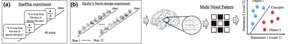
Exploring the mysteries of brain function is one of the most challenging and fascinating tasks in the domain of science. In recent years, with the advent of machine learning techniques, the interdisciplinary field of machine learning and neuroscience has drawn growing attention to both communities. With the aid of modern neuroimaging tech-niques, the capability of machine learning algorithms to identify distributed patterns of voxels in response to stimuli allows for decoding brain activities using data-driven models. A comprehensive review of previous studies has been provided in [1–3]. In this study, we would like to focus on multi-voxel pattern analysis (MVPA) [4], which is a commonly used methodological framework for analyzing functional magnetic resonance imaging (fMRI) data with machine learning algorithms (see Fig. 1). fMRI is a pop-ular, non-invasive neuroimaging technique to measure brain activity via blood-oxygen-level dependent (BOLD) signals, recorded as time series in a three-dimensional (3D) brain space. The precise spatial localization of brain acti-vation, therefore, is an essential advantage of fMRI com-pared to other non-invasive neuroimaging techniques. Unlike conventional univariate approaches, MVPA con-structs a pattern classification problem to decode neural information processing by characterizing multivariate brain activity patterns [5].
However, fMRI-based data analysis using machine learning approaches has a challenging small-n large-p problem, i.e., there are many thousands of voxels in the brain, but the sample size is relatively small because of the expensive cost of fMRI data collection. Moreover, only a portion of the brain will be activated with respect to specific stimulus or mental states. Hence, selecting the This research is supported in part by the Research Foundation for
SUNY Grant (award no: 66508) and the National Science Foundation (award no: 1538059)
M. FanC.-A. Chou (&)
Binghamton University, the State University of New York, 4400 Vestal Pkwy E, Binghamton, NY 13902, USA
e-mail: [email protected]
M. Fan
active voxels associated with particular stimuli or states is an important and challenging task before training classi-fiers in MVPA, which is calledfeature selectionorfeature reduction. In current studies, a common criterion of eval-uating the subset selection is classification accuracy. This evaluation criterion may suffer from the variance in training data with a limited sample size and result in unstable generalization error when the trained model is applied to an unknown dataset. Selecting stable features across various datasets, on the other hand, has not been completely investigated. Therefore, the objective of our study is to explore for an integrated stability-based feature selection approach.
The remainder of this paper is organized as follows: Section2 provides a brief review of existing studies, including stability selection algorithms and their applications to neuroimaging data. Section3illustrates the methodology, including experimental settings, data description, feature extraction and selection methods, classification algorithms, and methodological framework. Results are reported and discussed in Sect.4, followed by the conclusion and possible directions for future work in Sect.5.
2 Literature review
A major challenge in MVPA, as stated previously, comes from the high dimensionality and sparsity in fMRI data. Hence, the regularized logistic regression (LR) such as least absolute shrinkage and selection operator (LASSO) and elastic net (or ENet for short) are found to be partic-ularly useful in addressing sparsity. Another general objective of feature selection is to build inter-pretable models which are able to support or reject hypothesis with domain knowledge. To this end, selecting a stable subset that is robust to the variance in samples is of great importance. Numerous studies have discussed the stability issue using various types of feature selection methods from statistician’s perspective [6–9]. Numerous metrics to quantify the stability in feature selection were proposed, but no standard guideline for comparing various feature selection methods has been acknowledged up to
date [6,7,10,11]. In this section, a brief review of existing studies of stability selection is provided in terms of methodology and applications to neuroimaging data.
Before Meinshausen and Buhlmann [8] proposed their methodological framework of stability selection, some early studies have implied the usefulness of re-sampling strategy such as bootstrap of improving the stability of feature selection [7, 12]. In Meinshausen and Buhl-mann’s work, the subset selection is performed via repeatedly running LASSO on re-sampled subsets, while each subset is half the size of original samples. A feature is able to enter the model only if the frequency of being selected is greater than a user-defined threshold (denoted as H below). This method was later improved in [9] by changing the re-sampling mechanism such that if one half of the dataset was sampled, the other complimentary half should also be used. This Complimentary Pairs Stability Selection (CPSS) method has been mathemati-cally proved to provide an improved bound for the estimation error control. An interesting aspect of stability selection is that although original stability selection approach was claimed not to be sensitive to the selection ofHin a range of [0.6, 0.9], it was reported in the CPSS article [9] that the choice ofH may have an impact. In general, stability selection is a topic that has not been fully discovered.
Second, in terms of methodology, numerous variations were made utilizing the concept of stability selection. For example, the possible features for stability selection can be extracted from the functional network; in addition to voxels (or nodes in network science), selecting discriminative connectivity (edges) is also helpful to understand the mechanism underlying functional networks [13, 14, 18, 19]. Moreover, some studies integrated other machine learning algorithms such as clustering [15, 20, 21], graphical lasso [18], and support vector machine (SVM) [14]. A novel variation of LASSO was proposed to search for similar but not identical voxels in feature selection across multiple human subjects [22]. Finally, although the original stability selection was proposed as a data-driven model, some novel methods also utilized anatomical information, topological structure, or other structural information underlying features to enhance its stability and predictive power [16,23].
3 Methodology
3.1 Data description
Two benchmark datasets in cognitive science were used in our study: (1) StarPlus dataset [24] and (2) Haxby dataset [4].
3.1.1 StarPlus dataset
This dataset is named StarPlus because of the visual stimuli presented to subjects during the experiments. Subjects were instructed to focus on the visual stimulus on the screen when fMRI data was recorded. In one half of all experi-ment trials, a sentence (semantic stimulus) was presented first for 4 s (e.g., ‘‘It is true that the star is above the plus.’’), followed by an image (symbolic stimulus) showing similar information for another 4 s (see Fig.1a). The subjects need to press a button to indicate whether if the sentence and image matches each other. In remaining trials, the sequence of presenting sentences and images switches. 40 trials were conducted during this experiment, each of which contains 2 samples labeled by the type of stimulus (semantic = ‘0,’ symbolic = ‘1’).
The fMRI data was collected at 500 ms sampling rate in a 3D space of 64648 voxels, and the pre-processed data of 6 subjects is available to public. The scanned area contains 25–30 anatomical regions of interest (ROIs), which have approximately 4000 voxels. Particularly, 7 ROIs are highlighted by the proposer as they are most relevant to this task. Thus, the number of voxels to be analyzed in our study is reduced to around 2000, varying from subject to subject.
3.1.2 Haxby dataset
Haxby dataset contains the fMRI scans of 6 subjects. The experiment has 12 trials, each of which lasts for about 24 s, separated by rest periods (see Fig.1b). In each trial, 8 images presenting 8 types of objects including houses, human faces, cats, and so on. Images were shown on the screen for 500 ms of each; the inter-stimulus interval is 1500 ms. The entire experiment was then partitioned into 128¼96 samples from each individual with only one trial removed from subject 5 who was corrupted during this trial. The fMRI scans were collected in a space of 406464 voxels, corre-sponding to a voxel size of 3:53:753:75 mm3, and a volume repetition time of 2.5 s [4]. Similarly, instead of examining the whole brain, our study is focused on the visual cortex area which consists of up to 675 voxels based on the anatomical information of our subjects.
3.2 Feature extraction
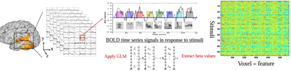
General linear model (GLM) approach as introduced in [25] was applied to the time series data for feature extraction. The basic concept is to characterize BOLD signals by fitting GLM to a haemodynamic response function (HRF) that describes blood-oxygen-level responses to the given stimu-lus as a function of time. The estimates of the coefficients
^
b¼ fb1; :::bmg T
in GLM model: Y ¼Xb represent the time-related response of each individual voxel to the stim-ulus of interest. Using b^as features results in an m-dimen-sional feature space, where each voxel is represented by its
beta value b^j;j2 f1; :::;mg. In our study, pre-processing and feature extraction were implemented in Matlab 8.3 [26] using a toolbox [27]. Figure2 illustrates extracting beta values as features for subject 1 in the Haxby dataset, where the samples (stimuli) are ordered in the same sequence as presented in the experiment.
3.3 Feature selection
Current feature selection methods are categorized into three classes based on how the subset-search algorithm is com-bined with the classification procedure: filter, wrapper, and embedded [28,29]. In this subsection, the selected feature selection methods are reviewed under this framework.
3.3.1 Filter approach
comprise the subset selection. In this study, Pearson cor-relation (referred to as Corr) and mutual information (MI) were employed as they are commonly used metrics. Moreover, the size of subset to be selected is not arbitrarily determined, but optimized using a cross-validation scheme. Since the classifier used in combination with these filter methods is SVM, these approaches will be referred to as SVM-MI, SVM-Corr in the following sections.
3.3.2 Wrapper approach
Instead of evaluating the similarity between individual fea-tures and class labels, wrapper methods seek for a best subset of features by evaluating the subset as a whole based on classification performance. The recursive feature elimina-tion (RFE) integrated with SVM, referred to as SVM-RFE, was chosen as an example of wrapper approach in our study. It is a backward feature selection approach which starts with the entire feature set and iteratively removes a propor-tion of features after evaluapropor-tion using SVM, which was implemented using a toolbox in Matlab 8.3 [30]. However, a significant disadvantage of wrapper methods is the compu-tational cost: the classification algorithm need to be per-formed repeatedly for every subset in the candidate pool, which will largely increase the computational time espe-cially with high-dimensional data. In order to be consistent with filter methods, the size of subset in feature selection was also optimized using a cross-validation scheme.
3.3.3 Embedded approach
The embedded methods utilize regression models with regularization. In such models, the feature selection is embedded in the training process of classification algo-rithm by optimizing a penalty parameter k. With an appropriatekselected using a cross-validation scheme, all redundant features are removed from the model by forcing their coefficients to be zero. In this study, we employ both LASSO and ENet as embedded approaches. More details about these algorithms are to be discussed later in Sect.3.4.
3.4 Classification algorithms
Consider that in a binary classification problem, the input data are a set of data points X¼ fx1; :::;xng in an m-di-mensional feature space, i.e., xi2 Rm8i 2 f1; :::;ng, wherenis the number of data points andmis the number of features. The corresponding target values T ¼ ft1; :::;tng are the class labels. The predictions of class labels are denoted byY¼ fy1; :::;yng. The objective of classification algorithms is to estimate the optimal parameters wandb, such that the mapping f :X!Y best captures the rela-tionship between inputs and targets.
3.4.1 Support vector machine
SVM is a classifier that optimizes the decision boundary with a maximum geometrical margin, i.e., the distance between decision boundary and the closest data points in each class. The soft-margin SVM with a linear kernel is formulated as follows:
arg min w;b
1 2kwk
2
þCX n
i¼1
ðniÞ; ð1Þ
s:t: tiðwTxiþbÞ 1ni 8i2 f1; :::;ng; ð2Þ
ni0 8i2 f1; :::;ng; ð3Þ
where slack variablesniare introduced to give tolerance to the misclassified data points lying in between support vectors, parameter Ccontrols the tolerance level, and the target values ti2 f1;1g. The decision boundary of a linear classifier is a hyperplane described by the function: fðxÞ ¼wTxþb, therefore for any data point i if fðxiÞ[0;yi¼1; otherwise yi¼ 1.
3.4.2 Regularized logistic regression
objective of LASSO is to find optimal solution for the following problem:
arg min w;b
X
jfðxiÞ tij2; ð4Þ
s:t:Xjwj k; ð5Þ
wherekis a tuning parameter which controls the shrinkage. This formulation can be generalized to logistic regression models by replacing Eq. (4) with the cost function in LR model. Similarly, the formulation of ENet shares the same objective function as in Eq. (4) but the constraint is as follows:
s:t:ð1aÞXjwj þaXjwj2k; ð6Þ
whereacontrols the trade-off between ridge regression and LASSO. In our study, a¼0:8 is used as a common selection.
3.5 Methodological framework
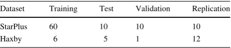
Although the concepts of stability selection were utilized in this study, the setup of experiment differs in two datasets. Table1 presents the cross-validation settings of both datasets. Let DT, DG; and DV denote training, test and validation set, respectively. The general framework is demonstrated as follows:
– Step 1: Randomly take a subsetDSout of training set DT;
– Step 2: Run the feature selection method on set DS while using DV to control the tuning parameters in selected algorithm;
– Step 3: Repeat step 1 and 2ntimes;
– Step 4: Use a set of most frequently selected features Sas the future feature set;
– Step 5: Train the model with selected features onDT andDV;
– Step 6: Evaluate the performance onDG;
– Step 7: Repeatedly perform Step 1 to 6 according to selected cross-validation scheme.
In Step 2, after specifying the DT, DG; and DV, the re-sampling was performed 50 times on DT for feature selection with simultaneous validation on DV. Provided
that stability selection method proposed a re-sampling scheme with embedded feature selection methods [8, 9], our approach was designed to utilize the filter and wrapper methods in the same manner such that the results can be compared apples to apples. Further, ten replications were conducted based on different settings ofDT,DG;, andDV for StarPlus dataset, while twelve replications were per-formed for Haxby dataset such that each trial was used exactly once as test set.
The stability measure in our study is Jaccard Index [33], a measure of similarity between two sets. Suppose there are two subsetsSaandSb, then the Jaccard Index for (Sa;Sb) is defined as
JCðSa;SbÞ ¼
jSa\Sb j
jSa[Sb j
; ð7Þ
wherejSjis the number of elements in setS.
When there are k subsets, the overall similarity is computed by averaging the pairwise Jaccard Index for all possible pairs. The formulation is given as follows:
JCk ¼ 2 kðk1Þ
X
a X
b6¼a
JCðSa;SbÞ: ð8Þ
4 Results and discussions
In this section, the results are presented and discussed from the following aspects. First, a comparison among selected feature selection methods is provided based on accuracy and stability. Second, the selection of H is further exam-ined to provide some suggestions for future studies. Finally, the localization of voxels selected by each method is discussed to provide some insights.
4.1 Feature selection methods
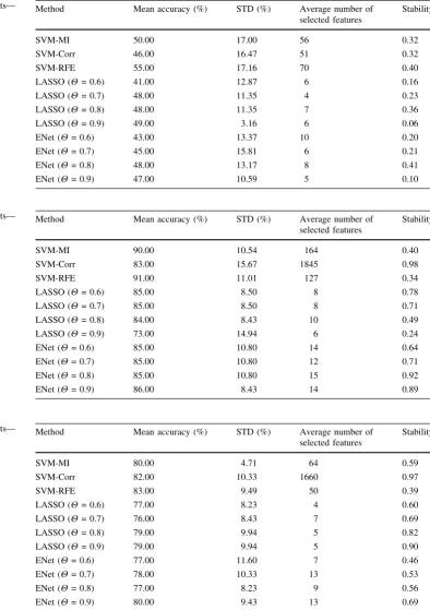
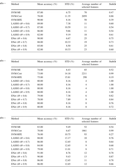
As shown in Tables2–13, the classification performance has a large variance across algorithms and subjects. In this sec-tion, some discussions are separately given to two datasets since algorithms performed differently in our experiment.
4.1.1 Filter and wrapper methods
In StarPlus dataset, SVM-MI, SVM-RFE, and SVM-Corr performed at a comparable level as embedded algorithms in terms of accuracy, but embedded algorithms yielded a better overall stability. Moreover, it is not desirable that SVM-Corr sometimes selected a large subset although it is always highly stable. It may imply that SVM-Corr approach, according to the current experiment settings, tends to overfit in some cases. In Haxby data, however, SVM-MI, SVM-RFE, and SVM-Corr algorithms are more accurate than embedded algorithms in general. In terms of Table 1 The cross-validation settings of datasets
Dataset Training Test Validation Replication
StarPlus 60 10 10 10
Haxby 6 5 1 12
computational cost, SVM-MI and SVM-Corr are much faster than SVM-RFE. Among these three algorithms, SVM-MI is suggested based on overall accuracy, stability, and computational time, which is interestingly consistent with a previous study using same dataset without utilizing stability selection [34].
4.1.2 Embedded methods
In general, ENet has higher stability and standard devia-tion compared to LASSO; also, it selects a larger and more stable subset. It indicates that throughout all repli-cations the ENet has more stable subsets in feature Table 2 Summary of results—
subject 04799 in StarPlus dataset
Method Mean accuracy (%) STD (%) Average number of
selected features
Stability
SVM-MI 50.00 17.00 56 0.32
SVM-Corr 46.00 16.47 51 0.32
SVM-RFE 55.00 17.16 70 0.40
LASSO (H= 0.6) 41.00 12.87 6 0.16
LASSO (H= 0.7) 48.00 11.35 4 0.23
LASSO (H= 0.8) 48.00 11.35 7 0.36
LASSO (H= 0.9) 49.00 3.16 6 0.06
ENet (H= 0.6) 43.00 13.37 10 0.20
ENet (H= 0.7) 45.00 15.81 6 0.21
ENet (H= 0.8) 48.00 13.17 8 0.41
ENet (H= 0.9) 47.00 10.59 5 0.10
Table 3 Summary of results— subject 04820 in StarPlus dataset
Method Mean accuracy (%) STD (%) Average number of
selected features
Stability
SVM-MI 90.00 10.54 164 0.40
SVM-Corr 83.00 15.67 1845 0.98
SVM-RFE 91.00 11.01 127 0.34
LASSO (H= 0.6) 85.00 8.50 8 0.78
LASSO (H= 0.7) 85.00 8.50 8 0.71
LASSO (H= 0.8) 84.00 8.43 10 0.49
LASSO (H= 0.9) 73.00 14.94 6 0.24
ENet (H= 0.6) 85.00 10.80 14 0.64
ENet (H= 0.7) 85.00 10.80 12 0.71
ENet (H= 0.8) 85.00 10.80 15 0.92
ENet (H= 0.9) 86.00 8.43 14 0.89
Table 4 Summary of results— subject 04847 in StarPlus dataset
Method Mean accuracy (%) STD (%) Average number of
selected features
Stability
SVM-MI 80.00 4.71 64 0.59
SVM-Corr 82.00 10.33 1660 0.97
SVM-RFE 83.00 9.49 50 0.39
LASSO (H= 0.6) 77.00 8.23 4 0.60
LASSO (H= 0.7) 76.00 8.43 7 0.69
LASSO (H= 0.8) 79.00 9.94 5 0.82
LASSO (H= 0.9) 79.00 9.94 5 0.90
ENet (H= 0.6) 77.00 11.60 7 0.46
ENet (H= 0.7) 78.00 10.33 13 0.53
ENet (H= 0.8) 77.00 8.23 9 0.56
selection, but these subsets yielded an unstablepredictive power compared to LASSO. Comparison based on the best performing model, ENet yields better accuracy than LASSO in general, which is also supported by previous study using the same dataset [35]. This phenomenon may
relate to the balance between variance and bias of gen-eralization error in statistics. The stability selection scheme provides a control to help avoid the situation of having an unstable feature subset in the model. On the other side, however, by reducing the total number of Table 5 Summary of results—
subject 05675 in StarPlus dataset
Method Mean accuracy (%) STD (%) Average number of
selected features
Stability
SVM-MI 87.00 6.75 70 0.47
SVM-Corr 78.00 11.35 2059 0.88
SVM-RFE 90.00 8.16 50 0.39
LASSO (H= 0.6) 89.00 7.38 11 0.60
LASSO (H= 0.7) 87.00 10.59 11 0.54
LASSO (H= 0.8) 86.00 9.66 11 0.54
LASSO (H= 0.9) 82.00 9.19 18 0.61
ENet (H= 0.6) 90.00 6.67 25 0.75
ENet (H= 0.7) 88.00 10.33 19 0.73
ENet (H= 0.8) 85.00 8.50 25 0.61
ENet (H= 0.9) 82.00 10.33 23 0.60
Table 6 Summary of results— subject 05680 in StarPlus dataset
Method Mean accuracy (%) STD (%) Average number of
selected features
Stability
SVM-MI 74.00 8.43 85 0.52
SVM-Corr 73.00 14.18 2211 0.99
SVM-RFE 75.00 15.81 298 0.19
LASSO (H= 0.6) 80.00 8.16 4 1.00
LASSO (H= 0.7) 80.00 8.16 4 1.00
LASSO (H= 0.8) 80.00 8.16 4 1.00
LASSO (H= 0.9) 80.00 8.16 4 1.00
ENet (H= 0.6) 79.00 7.38 6 0.82
ENet (H= 0.7) 78.00 7.89 9 0.84
ENet (H= 0.8) 80.00 8.16 8 0.76
ENet (H= 0.9) 80.00 8.16 8 0.72
Table 7 Summary of results— subject 05710 in StarPlus dataset
Method Mean accuracy (%) STD (%) Average number of
selected features
Stability
SVM-MI 83.00 9.49 52 0.54
SVM-Corr 70.00 6.67 1861 0.99
SVM-RFE 76.00 10.75 93 0.27
LASSO (H= 0.6) 88.00 13.17 10 0.76
LASSO (H= 0.7) 86.00 12.65 8 0.64
LASSO (H= 0.8) 84.00 12.65 9 0.68
LASSO (H= 0.9) 79.00 11.01 8 0.71
ENet (H= 0.6) 91.00 8.76 12 0.78
ENet (H= 0.7) 90.00 9.43 13 0.87
ENet (H= 0.8) 86.00 12.65 11 0.78
available samples for training purposes, it seems to scarify accuracy to some extent. This raises questions that, if it is possible to design a systematic approach to achieve or control the balance between stability and accuracy.
Depending on the objective of their studies, some researchers may favor an interpretable model to explore or support a hypothesis, while others may prefer a predictive one for practical use.
Table 8 Summary of results—
subject 1 in Haxby dataset Method Mean accuracy (%) STD (%) Average number ofselected features Stability
SVM-MI 90.63 12.07 122 0.70
SVM-Corr 84.38 16.96 338 0.58
SVM-RFE 84.38 16.96 219 0.49
LASSO (H= 0.6) 79.17 14.43 88 0.68
LASSO (H= 0.7) 77.08 13.93 75 0.67
LASSO (H= 0.8) 76.04 11.25 87 0.71
LASSO (H= 0.9) 71.88 16.10 95 0.61
ENet (H= 0.6) 38.54 26.36 255 0.71
ENet (H= 0.7) 59.38 20.03 235 0.70
ENet (H= 0.8) 62.50 21.98 255 0.67
ENet (H= 0.9) 80.21 11.25 232 0.67
Table 9 Summary of results—
subject 2 in Haxby dataset Method Mean accuracy (%) STD (%) Average number ofselected features Stability
SVM-MI 70.83 13.41 123 0.57
SVM-Corr 71.88 12.07 357 0.86
SVM-RFE 78.13 14.23 195 0.67
LASSO (H= 0.6) 55.21 6.44 94 0.57
LASSO (H= 0.7) 48.96 17.24 90 0.52
LASSO (H= 0.8) 48.96 17.24 97 0.46
LASSO (H= 0.9) 43.75 12.50 104 0.46
ENet (H= 0.6) 32.29 16.39 269 0.64
ENet (H= 0.7) 50.00 18.46 264 0.62
ENet (H= 0.8) 53.13 22.06 214 0.58
ENet (H= 0.9) 47.92 12.87 252 0.55
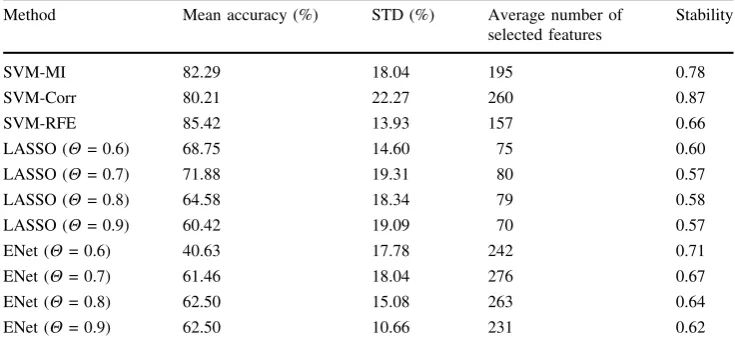
Table 10 Summary of results—subject 3 in Haxby dataset
Method Mean accuracy (%) STD (%) Average number of
selected features
Stability
SVM-MI 82.29 18.04 195 0.78
SVM-Corr 80.21 22.27 260 0.87
SVM-RFE 85.42 13.93 157 0.66
LASSO (H= 0.6) 68.75 14.60 75 0.60
LASSO (H= 0.7) 71.88 19.31 80 0.57
LASSO (H= 0.8) 64.58 18.34 79 0.58
LASSO (H= 0.9) 60.42 19.09 70 0.57
ENet (H= 0.6) 40.63 17.78 242 0.71
ENet (H= 0.7) 61.46 18.04 276 0.67
ENet (H= 0.8) 62.50 15.08 263 0.64
4.2 Threshold selection
According to the our experimental results, the selection of
H within [0.6, 0.9] has a significant influence on
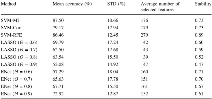
classification accuracy. This finding is consistent with the comments in [9]. More interestingly, a rough trend seems to imply that LASSO favors a smallerH while ENet pre-fers a larger one. As no previous studies have reported this Table 13 Summary of
results—subject 6 in Haxby dataset
Method Mean accuracy (%) STD (%) Average number of
selected features
Stability
SVM-MI 87.50 10.66 176 0.73
SVM-Corr 79.17 17.94 179 0.73
SVM-RFE 86.46 12.45 279 0.89
LASSO (H= 0.6) 69.79 17.24 42 0.60
LASSO (H= 0.7) 62.50 17.68 43 0.59
LASSO (H= 0.8) 63.54 15.50 39 0.52
LASSO (H= 0.9) 52.08 14.92 47 0.47
ENet (H= 0.6) 57.29 18.04 160 0.71
ENet (H= 0.7) 65.63 17.78 151 0.70
ENet (H= 0.8) 67.71 15.50 161 0.67
ENet (H= 0.9) 72.92 12.87 152 0.61
Table 11 Summary of results—subject 4 in Haxby dataset
Method Mean accuracy (%) STD (%) Average number of
selected features
Stability
SVM-MI 68.75 12.50 58 0.58
SVM-Corr 71.88 17.78 141 0.77
SVM-RFE 71.88 14.23 188 0.56
LASSO (H= 0.6) 56.25 22.30 30 0.52
LASSO (H= 0.7) 45.83 21.54 31 0.51
LASSO (H= 0.8) 42.71 22.90 28 0.36
LASSO (H= 0.9) 27.08 12.87 34 0.29
ENet (H= 0.6) 51.04 17.24 136 0.56
ENet (H= 0.7) 60.42 17.54 132 0.55
ENet (H= 0.8) 62.50 19.94 149 0.54
ENet (H= 0.9) 55.21 17.24 124 0.50
Table 12 Summary of results—subject 5 in Haxby dataset
Method Mean accuracy (%) STD (%) Average number of
selected features
Stability
SVM-MI 64.77 30.53 142 0.62
SVM-Corr 68.18 29.24 255 0.77
SVM-RFE 65.91 29.63 237 0.72
LASSO (H= 0.6) 51.14 24.01 24 0.58
LASSO (H= 0.7) 46.59 21.72 23 0.57
LASSO (H= 0.8) 39.77 22.23 21 0.43
LASSO (H= 0.9) 15.91 9.83 22 0.12
ENet (H= 0.6) 45.45 21.12 66 0.54
ENet (H= 0.7) 39.77 27.28 67 0.52
ENet (H= 0.8) 46.59 23.78 65 0.53
behavior in stability selection based on our knowledge, we can only make intuitive inference for the possible reason. Since group effect is encouraged in ENet, it tends to introduce more features into the model than LASSO, and thus a higherHis preferred to avoid introducing too many redundant features. Another interesting observation is the correlation to stability scores. For most subjects, the sta-bility scores seem to be negatively correlated with H in LASSO and ENet, which indicates setting up a high threshold may have a negative impact on model stability.
The size of subset to be selected after re-sampling and replications, however, does not show any correlations with
H in stability selection. Moreover, the size of subset remains stable in general for the same subject with a varying H. These findings encourage further exploration for standard guidelines for the selection ofH with empir-ical or theoretempir-ical supports.
4.3 Voxel selection and visualization
Figure3 presents a visualization of selected voxels for subject 1 in Haxby dataset and subject 04820 in StarPlus dataset. Subset selection is determined by picking up the most stable voxels, namely, the voxels with highest selection frequency throughout all replications. In general, the algorithms with higher stability scores: SVM-Corr, LASSO, and ENet selected a cluster of voxels located in visual cortex area, which is consistent with the domain-specific knowledge, while SVM-MI and SVM-RFE had a sparse voxel distribution. This indicates that stability-based feature selection framework provides a more stable, inter-pretable subset selection, which is difficult to achieve by evaluating models using accuracy.
5 Conclusion
In this study, we conducted a comprehensive analysis for a selection of filter, wrapper, and embedded feature selection approaches on the two benchmark fMRI datasets, adopting a stability-based methodological framework. It is found that the stability of feature selection is a potential alternative criterion for model selection in addition to classification accuracy, especially for those studies whose objective is to find a model with good interpretation rather than excellent predictive power. Having noticed that it is the case for the majority of neuroimaging data-based studies, developing stability-based feature selection may be helpful for identi-fying important voxels to decode mental states.
The future studies may explore a reliable metric to quantify the stability of feature selection methods because it has not been clearly defined. A standard guideline for selecting a suitable feature selection approach to achieve higher stability can be developed on the basis of a reliable metric. Also, a methodological framework which enables control of the balance between accuracy and stability is another issue to be further explored. Furthermore, it would be an interesting topic to examine the stability in voxel selection across different subjects, which will also be a challenging task because the activity patterns in brain are known to have large individual variations even in the same cognitive tasks.
Open Access This article is distributed under the terms of the Creative Commons Attribution 4.0 International License (http://crea tivecommons.org/licenses/by/4.0/), which permits unrestricted use, distribution, and reproduction in any medium, provided you give appropriate credit to the original author(s) and the source, provide a link to the Creative Commons license, and indicate if changes were made.
References
1. Haynes JD, Rees G (2006) Decoding mental states from brain activity in humans. Nat Rev Neurosci 7(7):523–534
2. Lemm S, Blankertz B, Dickhaus T, Mu¨ller KR (2011) Intro-duction to machine learning for brain imaging. Neuroimage 56(2):387–399
3. Pereira F, Mitchell T, Botvinick M (2009) Machine learning classifiers and fmri: a tutorial overview. Neuroimage 45(1):S199– S209
4. Haxby JV, Gobbini MI, Furey ML, Ishai A, Schouten JL, Pietrini P (2001) Distributed and overlapping representations of faces and objects in ventral temporal cortex. Science 293(5539):2425–2430 5. Norman KA, Polyn SM, Detre GJ, Haxby JV (2006) Beyond mind-reading: multi-voxel pattern analysis of fmri data. Trends Cognit Sci 10(9):424–430
6. Kalousis A, Prados J, Hilario M (2007) Stability of feature selection algorithms: a study on high-dimensional spaces. Knowl Inform Syst 12(1):95–116
7. Krˇizˇek P, Kittler J, Hlavac V (2007) Improving stability of fea-ture selection methods. Computer analysis of images and pat-terns. Springer, Berlin, pp 929–936
8. Meinshausen N, Bu¨hlmann P (2010) Stability selection. J Royal Stat Soc Ser B 72(4):417–473
9. Shah RD, Samworth RJ (2013) Variable selection with error control: another look at stability selection. J Royal Stat Soc Ser B 75(1):55–80
10. Kuncheva LI (2007) A stability index for feature selection. In: Artificial intelligence and applications, pp 421–427
11. Lim C, Yu B (2015) Estimation stability with cross validation (escv). J Comput Gr Stat (just-accepted)
12. Bach FR Bolasso: model consistent lasso estimation through the bootstrap. In: Proceedings of the 25th international conference on machine learning, pp 33–40. ACM (2008)
13. Liang X, Connelly A, Calamante F (2015) A novel joint sparse partial correlation method for estimating group functional net-works. Human Brain Mapp
14. Wang Y, Wu G, Long Z, Sheng J, Zhang J, Chen H (2013) Feature selection via sparse regression for classification of functional brain networks. Intelligence science and big data engineering. Springer, Berlin, pp 554–560
15. Bellec P, Rosa-Neto P, Lyttelton OC, Benali H, Evans AC (2010) Multi-level bootstrap analysis of stable clusters in resting-state fmri. Neuroimage 51(3):1126–1139
16. Wang Y, Zhang S, Zheng J, Chen H, Chen H (2015) Randomized structural sparsity-based support identification with applications to locating activated or discriminative brain areas: a multicenter reproducibility study. Auton Mental Dev IEEE Trans 7(4):287–300 17. Dresler T, Fallgatter AJ (2014) Scors—a method based on sta-bility for feature selection and apping in neuroimaging. IEEE Trans Med Imag 33(1)
18. Cribben I, Wager TD, Lindquist MA (2013) Detecting functional connectivity change points for single-subject fmri data. Front Comput Neurosci 7(143):10–3389
19. Ryali S, Chen T, Supekar K, Menon V (2012) Estimation of functional connectivity in fmri data using stability selection-based sparse partial correlation with elastic net penalty. Neu-roimage 59(4):3852–3861
20. Hoyos-Idrobo A, Schwartz Y, Varoquaux G, Thirion B (2015) Improving sparse recovery on structured images with bagged clustering. In: Pattern Recognition in NeuroImaging (PRNI), 2015 international workshop on, pp 73–76. IEEE
21. Varoquaux G, Gramfort A, Thirion B (2012) Small-sample brain mapping: sparse recovery on spatially correlated designs with randomization and clustering. arXiv preprintarXiv:1206.6447 22. Rao N, Cox C, Nowak R, Rogers TT (2013) Sparse overlapping sets
lasso for multitask learning and its application to fmri analysis. In: Advances in neural information processing systems pp 2202–2210 23. Gopakumar S, Tran T, Nguyen TD, Phung D, Venkatesh S (2015) Stabilizing high-dimensional prediction models using feature graphs. Biomed Health Inform IEEE J 19(3):1044–1052 24. Tom Mitchell, W.W.: Starplus fmri data.http://www.cs.cmu.edu/
afs/cs.cmu.edu/project/theo-81/www/.
25. Poldrack RA, Mumford JA, Nichols TE (2011) Handbook of functional MRI data analysis. Cambridge University Press, Cambridge
26. MATLAB (2014) version 8.4 (R2014a). The MathWorks Inc., Natick, Massachusetts
27. Kampa K.: fmri preprocessing toolbox.https://sites.google.com/ site/kittipat/mvpa-for-brain-fmri/fmri-data-preprocessing/beta-extraction-version-1-8
28. Mwangi B, Tian TS, Soares JC (2014) A review of feature reduction techniques in neuroimaging. Neuroinformatics 12(2): 229–244
29. Saeys Y, Inza I, Larran˜aga P (2007) A review of feature selection techniques in bioinformatics. Bioinformatics 23(19):2507–2517 30. Yan K, Zhang D (2015) Feature selection and analysis on
cor-related gas sensor data with recursive feature elimination. Sens Actuators B 212:353–363
31. Tibshirani, R.: Regression shrinkage and selection via the lasso. Journal of the Royal Statistical Society. Series B (Methodologi-cal) pp. 267–288 (1996)
32. Zou H, Hastie T (2005) Regularization and variable selection via the elastic net. J Royal Stat Soc Ser B 67(2):301–320
33. Real R, Vargas JM (1996) The probabilistic basis of Jaccard’s index of similarity. Syst Biol 45:380–385
34. Chou CA, Kampa K, Mehta SH, Tungaraza RF, Chaovalitwongse WA, Grabowski TJ (2014) Voxel selection framework in multi-voxel pattern analysis of fmri data for prediction of neural response to visual stimuli. Med Imag IEEE Trans 33(4):925–934 35. Kampa K, Mehta S, Chou CA, Chaovalitwongse WA, Grabowski TJ (2014) Sparse optimization in feature selection: application in neuroimaging. J Glob Optim 59(2–3):439–457
Miaolin Fan is currently a Ph.D. student at SUNY Binghamton, where she completed her master degree. Prior to her graduate study, she earned her bachelor degree in psychology. Her research interests lie in the interdisciplinary field of cognitive science and artificial intelligence. She primarily focuses on machine learning techniques in brain research with various neuroimaging data, particularly address-ing a typical ‘‘small-n-large-p’’ problem in neuroimagaddress-ing data with regularization methods.