O R I G I N A L A R T I C L E
Open Access
Labour supply and income distribution effects of
the working income tax benefit: a general
equilibrium microsimulation analysis
Nabil Annabi
*, Youssef Boudribila and Simon Harvey
* Correspondence:
[email protected] Policy Research Directorate, Human Resources and Skills Development Canada, Gatineau, Canada
Abstract
In this study we assess the impact of the Working Income Tax Benefit (WITB) on labour supply, GDP and income distribution in Canada, using a general equilibrium microsimulation model. We also estimate labour supply and demand elasticities using survey data to ensure that households’behaviour is properly captured in the model. Simulation results show that the WITB affects particularly labour market participation of low- and medium-skilled lone-parents families. These positive effects on labour supply translate into higher after-tax incomes leading to a decline in low-income rates and low-income gaps. Our findings suggest that enhancing the WITB could provide additional income support to working Canadian families while reducing work disincentives for those trapped behind the welfare wall.
JEL classification:C15, D33, D58, J08, I32, O51
Keywords:General equilibrium; microsimulation; elasticities; labour supply; income distribution; Canada
1. Introduction
In 2007 the federal government introduced a new work incentive, the Working Income Tax Benefit (WITB), to encourage individuals to enter the workforce and to reduce pressures on social programs. In the 2009 Federal Budget, the WITB was boosted in order to double the fiscal relief. With a budget of $1.135 billion in 2009–10, more than 1.5 million Canadians are targeted to benefit from the enhanced WITB. Although the total budget allocated to this program is modest, this earning supplement may entail significant work incentives and distributional effects at the household level. Indeed a number of studies that have examined the impact of similar earning supplements–in partial equilibrium framework–suggest that they are likely to have positive effects on labour supply and poverty alleviation. However, what would be the impact of these work incentives on net labour supply if general equilibrium effects are taken into ac-count? And what would be the impact of a rise in labour supply on low-income earners when indirect effects, such as a decline in wage rates, are accounted for? In an attempt to provide answers to these questions, we conduct policy simulations with a newly developed general equilibrium model with nearly 30,000 families to assess the net impact of this refundable tax credit on households’ labour market participation, low-income families and income distribution. In addition, to ensure that households’
© Annabi et al.; licensee Springer. This is an open access article distributed under the terms of the Creative Commons Attribution License (http://creativecommons.org/licenses/by/2.0), which permits unrestricted use, distribution, and reproduction in any medium, provided the original work is properly cited.
behaviour is properly captured in the model, we have empirically estimated labour sup-ply elasticities by household composition and income bracket for model calibration.
Three scenarios are simulated taking into account increased work incentives for low-income earners (Scenario 1), labour market participation of social assistance recipients (Scenario 2), and the risk of higher marginal tax rates when this tax credit is phased-out (Scenario 3). At the aggregate level, the results show positive but modest impacts on labour supply and GDP, as well as a decline in low-income rates and income inequality. At the micro level, the shocks affect particularly labour market participation of low- and medium-skilled lone-parent families. These positive effects on labour supply translate into higher after-tax incomes leading to a decline in low-income rates and low-income gaps. Regarding the impact on inequality (as measured by the Gini index), we find a decline across all household categories, especially lone parents. Finally, robustness analysis is per-formed showing that the declines in the low-income rate and inequality at the aggregate level are statistically significant only under Scenarios 1 and 2. Nevertheless, the results show that all three scenarios lead to an alleviation of the low-income gap (as measured by the amount of money by which each household falls below the low-income threshold).
We present a brief literature review on income supplements in Section 2. Sections 3 and 4 describe the main features of the model and the data used for its calibration. Policy simulations and analysis are discussed in Section 5. Finally, Section 6 concludes.
2. Literature review
In this section we briefly review the antecedents to the WITB, such as the Earned Income Tax Credit (EITC) in the US and the Working Tax Credit (WTC) in the UK1. We also summarise key research findings and discuss existing Canadian studies that have examined the potential impact of earning supplements on labour supply and poverty alleviation.
increase in the employment of single parents is attributable to the EITC. Furthermore, a number of studies have focused on evaluating labour supply responses to the EITC at the extensive (participation) and intensive (hours worked) margins. The findings of Meyer (2002) suggest that labour supply adjustment of single mothers mainly occur at the exten-sive margin. At the intenexten-sive margin, the EITC clearly encourages single parents to work in the phase-in portion. On the plateau, and particularly over the phase-out range, a labour supply disincentives should exist and should lead to a reduction in the hours worked. However, the author concludes that this latter effect is rather unclear. Eissa and Hoynes (2005) discuss different factors that may explain this issue. In most cases work schedules may be rigid, and workers often ignore the structure of the EITC schedule. Be-sides, the empirical literature on labour supply suggests that the elasticities may be higher at the extensive than at the intensive margin.
On the other hand, the British government introduced in the late 1990s a series of policy reforms in order to reduce child poverty and to increase employment of families with children. These reforms include the New Deal for Lone Parents (NDLP) intro-duced in 1997–1998 and the Working Family Tax Credit (WFTC) enacted in 1999. The WFTC was replaced in 2003 by two new tax credits: the Child Tax Credit (CTC) and the Working Tax Credit (WTC). The WTC is accessible to employed and self-employed persons and aims to make work pay for low income workers. The program is complex and differs according to worked hours, childcare allowances, disability, and age. There is no phase-in range, but the credit is available only to those working at least 16 hours per week. Besides, the phase-out rate is steep leading to high effective mar-ginal tax rates. Returns from the WTC program are delivered with each pay and are considered as revenues. The impacts of these policy reforms have been examined in a number of studies. Brewer (2003), Gregg and Harkness (2003), Blundell and Hoynes (2004), Francesconi and van der Klaauw (2004), Brewer et al. (2005), Leigh (2005), and Brewer et al. (2010) conclude that these reforms usually lead to a positive impact on labour force participation and labour supply, especially for single mothers. However, the impact on the labour supply of secondary earners of couple families may be nega-tive when their earnings are over a certain threshold.
At the provincial level, Brouillette and Fortin (2008) use an experimental approach to examine the impacts of the working premium in Quebec (Prime au Travail) on work effort of one person and lone parent families. The participants were asked in the exper-iments to perform various tasks under some constraints representing different tax re-gimes. The authors conclude that individuals respond positively to the working premium fiscal incentives. They also suggest that final conclusions can only be obtained with a general equilibrium model. The more recent study of Moffette et al. (2013) esti-mates the impacts of the Quebec working premium using a microsimulation approach4. The authors find a positive impact on aggregate labour supply, with the variation at the extensive margin being more important than at the intensive margin. They also show that labour supply increases for both men and women but it decreases at the intensive margin for lone parent women.
the enhanced WITB. Although the total budget allocated to the program may seem modest, this earning supplement could produce substantial work incentives and distri-butional effects. To our knowledge there is no existing study analysing the labour mar-ket and income distribution impacts of the WITB. In the present research paper, we fill this literature gap by developing a microsimulation general equilibrium model to simu-late the impacts of this in-work tax credit on employment and low-income families. This methodology is very appropriate as it enables assessing the impact on labour sup-ply and income at the family level while taking into account general equilibrium effects on wages. In addition, we estimate labour supply and demand elasticities for 25 house-hold categories to ensure that househouse-holds’behaviour is properly captured in the model.
3. Model features
We develop an integrated microsimulation computable general equilibrium (CGE) model that draws on the contribution of Cockburn (2001) and Annabi et al. (2005), Annabi et al. (2008), Annabi et al. (2013). The combination of general equilibrium aspects with the de-tailed information provided by the microsimulation technique allows us to better assess the impact of policy reforms on labour markets and income distribution6. The model is calibrated with Canadian data for 2003. Matching and balancing (data reconciliation) techniques are used to integrate the 29,846 economic families from the Survey of Labour and Income Dynamics (SLID) into the general equilibrium framework. The integrated framework employed is preferred to other approaches for linking CGE models with survey data since it ensures that feedback effects from the micro level are fully captured at the macro level. In the following we briefly describe the model characteristics7.
The analysis of policy simulations at the household level involves modeling sectoral labour and capital markets which allow a better assessment of general equilibrium ef-fects on wages and investment income8. The CGE the model includes 12 sectors pro-ducing 17 products (goods and services) based on the Input–output (IO) tables from Statistics Canada. Only 14 out of these 17 products are directly consumed by house-holds. In each sector, the production of goods is represented by a Constant Elasticity of Transformation (CET) function. This reflects the rectangular aspect of the IO tables where each sector supplies more than one good depending on relative market prices. Also, we adopt a nested structure for the production technology. Sectoral gross output is a Leontieffunction of value-added and total intermediate consumption. Value-added is in turn represented by a Cobb-Douglassfunction of capital and aggregate labour fac-tor which is represented by a Constant Elasticity of Substitution (CES) function of three skill levels: high-, medium-, and low-skilled workers according to the National Occupa-tional Matrix (NOC)9. Labour is assumed mobile between sectors, whereas capital is sector-specific and is only mobile through new investments.
Households also earn labour income and receive transfers from the government and from the rest of the world. They pay direct income tax to the government and transfers to foreigners. Preferences of the 29,846 households modelled are represented by a Stone-Geary function with minimum consumption of goods and leisure. Hence, utility maximisation yields an Extended Linear Expenditure System (ELES) with an endogen-ous labour supply equation for each skill level within each hendogen-ousehold. Hendogen-ousehold sav-ings are characterised by a positive marginal propensity to save and a fixed intercept that may be positive or negative. This specification allows initially negative savings to become positive after a given threshold.
For a realistic representation of the Canadian economy, a foreign sector is also in-cluded in the model to represent external trade. This feature allows us to better capture the impact of foreign savings on capital accumulation, hence long-term effects of policy shocks. We assume that foreign and domestic goods are imperfect substitutes. This geographical differentiation is introduced by the standard Armingtonian assumption with a CES function between imports and domestic goods. On the supply side, pro-ducers make an optimal distribution of their production between exports and domestic sales according to a CET function. We also assume a finite elasticity export demand function. In order to increase their exports, local producers must decrease their free on board (FOB) prices.
The public sector is represented by the federal government and a consolidated pro-vincial and local government. Both governments collect direct tax revenues from households and firms and indirect tax revenues on domestic and traded goods and ser-vices. Public expenditures are allocated between the consumption of goods and services and transfers. In each period the former component of public expenditures is adjusted to respect a long-run closure rule consisting in fixed ratios of public saving to GDP. In addition, we assume that foreign savings are also fixed in proportion of GDP10.
The model includes a dynamic module where capital stock is updated with a standard capital accumulation equation involving capital depreciation rate and investment by destin-ation. The latter is represented by an investment demand function which determines how new investments will be distributed between sectors. This function is similar to that pro-posed by Jung and Thorbecke (2003). In each sector, the capital accumulation rate–ratio of investment to capital stock–is an increasing function of the ratio of the rate of return to capital and its user cost11. The latter is equal to the dual price of investment (capital good price) times the sum of the depreciation rate and the exogenous real interest rate.
In addition, the dynamic updating of the model includes price-indexed nominal variables such as transfers, and exogenous volumes such as external demand for Canadian exports12. The model is homogenous in prices and calibrated to generate a steady state where all var-iables remain constant, which facilitates the counterfactual (i.e., simulated scenario) distri-butional analysis13. Finally, general equilibrium is defined by the equality (in each period) between supply and demand of goods and factors, and the savings-investment identity. The nominal exchange rate is chosen as the numéraire in each period.
4. Model calibration
4.1. Data preparation
2001 Census data14. The latter is used for sectoral labour income disaggregation by skill level according to the National Occupational Classification (NOC) matrix15. The data for the 29,846 economic families integrated in the CGE model are based on the 2003 SLID. This survey contains detailed information on income sources, and taxes and transfers at both the economic family and personal level. Besides, the SLID sample of 57,233 individuals may be linked to the economic family sample using families’ identi-fiers. The link between the two samples allows disaggregating each household labour income by skill level using information on occupations and the number of years of edu-cation of the household members included in the person file.
The SLID also includes information on age, household composition, province of resi-dence, and sector of activity. However, it has a shortcoming in that it does not include information on the consumption of goods and services. To obtain detailed information on expenditures we turn to the 2003 Survey of Households Spending (SHS), which lacks detailed information on income sources, and employ matching techniques (see Abadie et al. 2001) to impute consumption vectors (products) to the SLID economic families16. First, for a given SLID observation the matching generates total consump-tion as a funcconsump-tion of specified household characteristics (e.g., adjusted adult-equivalent after-tax income, size, age of reference person, province and size of region of residence) in both the SLID and the SHS. Second, total expenditure is then disaggregated into the consumption of various goods and services assuming that the SLID family has the same preferences as its analogous (match) family in the SHS. Finally, as a measure of robust-ness of the results, we compared the estimated distribution of total consumption (gen-erated by the matching procedure) to the observed SHS distribution by computing several income distribution indices. The similarity of both the shape of the distributions and the various statistical indices supports the outcomes of the procedure employed. Indeed, the differences in low-income rates and Gini indices computed with the two distributions are found to be less than one percentage point.
Moreover, we have to produce a macro–micro consistent data set for the implemen-tation of the model. The comparison of the totals of income and consumption vectors at the micro level with those in the SAM reveals an undervaluation in survey data rela-tive to the national accounts, which may be explained by underreporting. This implies that we must reconcile these differences. To keep the structure of the economy un-changed, we adjust household data to meet the national accounts totals. To adjust households’consumption and income components, we minimise the cross entropy di-vergence measured by the Kullbak-Leibler function, as in Robilliard and Robinson (2003), subject to the constraint of equality between the SAM cells and the total weighted household observations values. Other minimisation criteria, such as the standard sum of squared differences, were also tested and compared, but did not per-form better.
technique implemented here yields a good approximating distribution, denoted “ Bal-anced”, of the“raw”distribution of net income in the survey data.
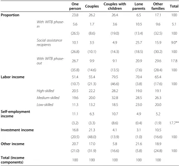
Households’ income composition based on the balanced data set is reported in Table 1. It shows that factor income, especially labour, represents the largest source of income for all households categories (One person, Couples, Couples with children, Lone parents, and Other families)17. Let us focus on Couples and Lone parents families. With a proportion of 26.2 percent in total population, Couples without children earn 55.4 percent of their income from labour especially high-, and medium-skilled labour. The second source of income by declining order of importance is capital income (i.e., investment income plus self-employment income) which represents over 27 percent of total income. Capital income includes investment income and self-employment income. Almost 50 percent of total investment income (including pensions and registered re-tirement saving plans withdrawals) in the economy is accruing to Couples. Regarding Lone parents, their primary source of income is also labour income, which represents more than 70 percent of total income, and they earn most of this income from medium- and low-skilled occupations. In addition, Lone parents have higher shares of households with incomes in the phase-in of the WITB and receiving social assistance benefits. Consequently, we may expect that the simulation of the WITB will lead to a more pronounced labour supply response among low-skilled Lone parent families in comparison with Couples.
4.2. Estimation of households’preferences
As previously mentioned, households’ preferences are represented by a Stone-Geary utility function with minimum consumption of goods and leisure, which yields an ELES with a labour supply function18. The ELES has the attractive property of accommodat-ing non-unitary income elasticities of demand but its use in CGE models involves a
0
0 30,000 60,000 90,000 120,000
(Dollars)
Raw data – FGTo = 12.61%
Simplydistributed – FGTo = 11.18% Balanced – FGTo = 12.57%
.00001 .00002 .00003
–
– –
Figure 1Density curves of adult-equivalent net income. Notes:FGTo denotes the share of households with income below the low-income measure which equal to fifty percent of median income. In this figure,
number of estimated parameters. Indeed, the calibration of this system requires the values of income elasticities of demand, income elasticities of labour supply, and the Frisch parameter19. The Frisch parameter is defined as the negative value of the ratio of total consumption (or disposable income) to discretionary consumption (i.e., total con-sumption minus minimum concon-sumptions) and is used to derive values for minimum consumptions. To our knowledge, there is no existing empirical research addressing the question of how different Canadian household categories jointly allocate their leis-ure time and expenditleis-ures across seemingly unrelated commodities that are ultimately interconnected through their budget constraints20. In addition, the short-run behaviour represented by the cross-sectional data indicates non-consumed goods and zero labour supply (income) for many families. While most existing empirical studies completely isolated labour supply analysis, or joined leisure to a consumption of an aggregated good, we implement an approach that allows us to take into account corner solutions (i.e., non-consumed goods and zero labour supply)21. According to Kao et al. (2001), ap-proaches previously used are not appropriate to study the short-run price response of
Table 1 Base run distribution of households and income sources
One
person Couples
Couples with children
Lone parents
Other families Total
Proportion 23.8 26.2 26.4 6.5 17.1 100
With WITB
phase-in 5.6 1.7 3.6 10.5 9.6 5.1
(26.5) (8.6) (19.0) (13.4) (32.5) 100
Social assistance
recipients 10.1 3.5 4.9 25.7 15.9 9.0*
(26.8) (10.1) (14.3) (18.5) (30.2) 100
With WITB
phase-out 26.7 9.9 9.1 20.9 29.6 17.8
(35.8) (14.6) (13.5) (7.6) (28.4) 100
Labor income 51.4 55.4 79.5 70.4 65.4
(10.7) (21.3) (46.6) (3.8) (17.6) 100
High-skilled 20.5 22.2 28.2 19.0 19.1
Medium-skilled 19.6 20.0 32.8 28.5 26.3
Low-skilled 11.3 13.2 18.5 23.0 20.0
Self-employment
income 11.1 6.3 10.7 4.9 5.2
(3.2) (3.3) (8.6) (0.4) (1.9) 17.7**
Investment income 16.8 21.3 4.1 3.1 10.5
(20.5) (48.0) (13.9) (1.0) (16.6) 100
Other income 20.7 17.0 5.8 21.6 18.9
(21.0) (31.9) (16.6) (5.8) (24.8) 100
Total (income
components) 100 100 100 100 100
Source: Authors’calculations.
Note: See section5for more details on the phase-in and phase-out of the WITB. Figures in brackets represent the share in population or in total factor income.
* The proportion of families that receive social assistance benefits and are able to enter the labour market under certain conditions is only about 2.3 percent (see Table3and Scenario 2 below).
consumer behaviour22. In an ELES with binding non-negativity constraints, a corner solu-tion for a given good can occur only if the minimum consumpsolu-tion of that good is negative or zero (i.e., unnecessary good). In the case of zero labour supply, the time available for market work is equal the maximum available time less the time for minimum leisure.
For each household type, we obtain a system of 13 equations of commodities and one equation of labour supply. The obtained econometric model is a seemingly unrelated re-gression with censored data (Zellner 1962). We drop one equation because of the linearity condition on the coefficients of the model and derive the corresponding likelihood func-tion that takes into account the zeros in consumpfunc-tion and labour supply. The result is a multidimensional integral likelihood function. We adapt the algorithm of a simulated maximum likelihood (SML) function proposed by Kao et al. (2001) to our case. The pro-cedure uses the Geweke-Hajivassiliou-Keane (GHK) simulator developed by Geweke (1991), Börsh-Saupan, and Hajivassiliou (1993), Hajivassiliou and McFadden (1990), and Keane (1994). Compared to the existing SML and Bayesian methods (Markov Chain Monte Carlo, MCMC), the GHK appears to be robust and more efficient in terms of com-putational time. The GHK simulator evaluates the probability each individual contributes to the likelihood function. It switches back and forth between computing univariate trun-cated normal probabilities, simulating draws from univariate normal distributions, and computing normal distributions conditional on previously drawn truncated normal ran-dom variables. We simulate 5,000 draws from univariate normal distributions. The itera-tive maximum likelihood estimations require large amounts of time to approximate the global maximum, especially in cases where the data presents areas of little variation (plat-eau). We used the analytically derived gradient when the numerical computation time was problematic23. At the computational level, we parametrise the minimum consump-tion to ensure the positive value of virtual prices24, and take into account the frequencies of the zero observations for each consumed good and labour supply within each group of households. This allows us to avoid considering unnecessary goods for a small proportion of the population in each group, as unnecessary for the whole group (i.e., consumptions of the good by all households are equal to zero). Finally, we used the estimated parameters to derive marginal shares and income elasticities25.
To estimate the income elasticities of demand and labour supply and Frisch parame-ters we consider five income brackets and the same household categories discussed above. We also exclude households with a major income earner aged 65 plus. We then obtained 24,213 households of the 29,846 economic families of the microsimulation model. The data shows that, for each household, the higher the income per person, the more diversified is the basket of the consumed goods. Table 2 presents the estimated income elasticities of labour supply for the linear expenditure system evaluated at the sample mean by household composition and income brackets. Values of income elasti-cities of demand and the Frisch parameters are provided in the Appendix.
Estimation results in Table 2 are consistent with economic theory and are in line with previous findings in the literature on labour supply elasticities obtained with various functional forms and approaches. According to the review by Blundell and MaCurdy (1999) the range of income elasticities of labour supply in the literature is −0.95 to
lower income families, i.e., when at the extensive margin, and the maximum is for Lone parent households (−0.39). Household’s labour supply elasticity decreases in absolute value with income. This implies that the reaction to an increase in income tends to be larger for households at the extensive margin than for households at the intensive mar-gin. The income elasticity is lower in absolute value for all households with income higher than $55,000, (i.e., at the intensive margin) and reaches 0.05.
Regarding income elasticities of demand, the findings are consistent with the under-lying theoretical model. Depending on the various income brackets, the considered es-sential goods have elasticities less than one, while the ineses-sential goods and the luxury goods have elasticity larger than one. In contrast, the Frisch parameters provide a new insight about the minimum consumption behaviour of lower-income households. When the Frisch parameter is near unity in absolute value, minimum consumption of some goods may be nil or negative. In the latter case the good is deemed unnecessary (Kao et al. 2001). This implies that almost all their income is spent on the consumption of basic needs. In fact, model calibration reproduced the negative values for minimum consumptions of non-consumed products for some households. Nevertheless, the esti-mated Frisch parameters for higher income families are around −1.2, indicating that minimum consumption is around 20 percent.
5. Policy simulations and results
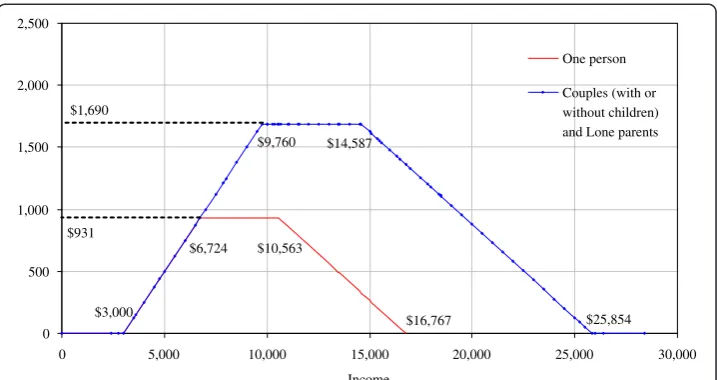
The configuration of the WITB may differ according to family status, provinces and dis-ability conditions. Provinces and territories have the flexibility to redesign or harmonise the WITB according to their own income security programs and policies. However, varia-tions in its design must respect several rules such as improving work incentives for low-income earners and being cost-neutral to the Federal government. Figure 2 presents the parameters of the WITB for One person households, Couples and Lone parents. The credit starts after a threshold of $3,000 to ensure a minimum attachment to the labour market and increases at a phase-in rate of 25 percent of each dollar of earned income up to the maximum benefit. The maximum benefit is granted for incomes between $6,724 and $10,563 (the plateau) for One person households and for income between $9,760 and
Table 2 Income elasticities of labour supply by household category
One person Couples Couples with children Lone parents Other families
Less than $15,000 −0.140 −0.263 - −0.399 −0.206
(0.004) (0.010) - (0.020) (0.008)
$35,000 to $55,000 −0.159 −0.135 −0.265 −0.249 −0.116
(0.001) (0.002) (0.003) (0.004) (0.002)
$55,000 to $100,000 −0.099 −0.062 −0.066 −0.086 −0.091
(0.001) (0.000) (0.000) (0.000) (0.001)
$100,000 to $150,000 −0.050 −0.064 −0.056 −0.079 −0.072
(0.001) (0.001) (0.000) (0.002) (0.001)
More than $150 - −0.062 −0.078 - −0.081
- (0.000) (0.001) - (0.001)
Source: Estimation results.
$14,587 for Couples (with or without children) and Lone parents. Then, the benefit starts to phase-out at a rate of 15 percent of each additional dollar. In order to simulate the effects of the WITB, its parameters have to be translated in terms of changes in marginal tax rates.
An example of the impact of the WITB on the effective marginal tax rate (EMTR) is pre-sented in Figure 3a and b. It shows how the EMTR decreases or increases depending on whether the income is in the phase-in or the phase-out of the tax credit. Marginal tax rates for persons with incomes in the plateau should remain unchanged. On the other hand, given that the WITB is calculated on a personal basis (except for couples), the SLID per-sonal file has been used to adjust tax rates at the family level. For example, a person aged 19 years, living with his parents and is not a full-time student is eligible for the WITB. We have used weighted average of EMTR to account for similar cases26. As the introduction of the WITB requires a financing source to maintain budget equilibrium, we assume in the following scenarios that public expenditure on goods and services is adjusted to main-tain a fixed ratio of government saving to GDP. In addition, we assume a take-up rate of 100 percent where all households entitled to the WITB would claim the benefits27.
– Scenario 1: Simulates work incentives for low-income earners taking into account only the phase-in of the WITB with a decline in EMTR with respect to the base run.
– Scenario 2: Scenario 1 + increased labour market participation of social assistance recipients as low-skilled workers.
– Scenario 3: Scenario 2 + risk of higher EMTR in the phase-out of the WITB.
In the simulations, social assistance recipients that are able to work must have no, Canada/Quebec Pension Plan (C/QPP) income, or Old Age Security (OAS) and Guar-anteed Income Supplement (GIS), be 19 years or older, and enter the labour market as low-skilled. Table 3 presents the percentage of social assistance recipients able to enter the labour force by province. We use these proportions to calibrate the labour supply function of persons with initially zero labour supply (income), which is activated only under Scenarios 2 and 3. The procedure used for the calibration of households with initially zero labour supply is similar to that proposed by Fortin et al. (1993).
$16,767 $10,563
$931
$25,854 $3,000
$6,724 $1,690
$14,587 $9,760
0 500 1,000 1,500 2,000 2,500
0 5,000 10,000 15,000 20,000 25,000 30,000
Income
One person
Couples (with or without children) and Lone parents
In the model, changes in EMTR affect both federal transfers to households – hence after-tax income–and the opportunity cost of leisure (net wage rate). The net impact on labour supply will depend on the magnitude of these two effects. If the income ef-fect is smaller than the price (substitution) efef-fect, the consumer reacts to a rise in the net wage rate by reducing leisure and increasing time devoted to work. In the opposite situation, labour supply declines.
5.1. Aggregate effects
Table 4 presents the aggregate impacts on key indicators in percentage change from the base run. As expected, the results show that the impacts of the WITB on aggregate labour supply and GDP are positive but modest. The largest changes are obtained under Scenario 2 when the potential work of social assistance recipients is accounted for. Under Scenario 3, however, both labour market participation and GDP are hardly affected since households with benefits phase-out are taken into account in the simulation.
0 0.2 0.4 0.6 0.8 1
0 10000 20000 30000 40000
E
ff
e
ct
iv
e M
a
rg
in
al
T
a
x
R
a
te
Income (dollars)
Including WITB Excluding WITB
0 0.2 0.4 0.6 0.8 1
0 10000 20000 30000 40000
E
ff
e
ct
iv
e M
a
rg
in
al
T
a
x
R
a
te
Income (dollars)
Including WITB Excluding WITB
a
b
The positive impact on labour supply translates into relatively lower wage rates, par-ticularly for low-skilled workers who are primarily targeted by work benefits30. These changes in real wages could not be captured in a partial equilibrium framework. This may affect the evaluation of policy reforms because labour supply depends not only on income but also on the wage rate net of marginal tax rates. Furthermore, the higher in-crease in labour market participation under Scenario 2 leads to a more pronounced de-cline in low-income rates and income inequality as measured by the Gini index31. The outcomes are different under Scenario 3, with a marginal increase in the low-income rate and a decrease in the low-income gap. The slight increase in wage rates of high-and medium-skilled workers is due to a negative impact on labour supply. To examine how the shock has led to the above changes in low-income rates and inequality, Figure 4 plots the cumulative change in income by percentile. The negative slope of the depicted curves implies that the shock benefits relatively more low-income families. Moving from the left to the right more changes in income are added leading to a decline in these curves which suggest that the new changes being added are smaller or in some cases negative. The last points located on the curves are the average changes in income.
Table 3 Potential labour supply of social assistance recipients, percent
Work potential Persons with long-term disability
Newfoundland and Labrador 78 22
Prince Edward Island 47 53
Nova Scotia 54 46
New Brunswick 76 24
Quebec 64 36
Ontario 47 53
Manitoba 43 57
Saskatchewan 33 67
Alberta 54 46
British Columbia 41 59
Canada 53 47
Source: HRSDC (2010), Social assistance statistical report.
Note: Proportions of work potential are distributed across households to scale down labour supply response (by reducing the maximum time available for work) in order to avoid overestimating the positive effects of the WITB. Consequently, the proportion of families receiving SA benefits accounted for in the simulation (Scenario 2) is reduced from 9 percent to 4.3 percent when the conditions on non-labour incomes and age are respected, and to only 2.3 percent when persons with long-term disability are dropped from the sample.
Table 4 Aggregate effects, percentage change from the base run29
Scenario 1 Scenario 2 Scenario 3
Labour supply 0.15 0.21 0.04
Real GDP 0.09 0.12 0.02
Wage rate
High-skill −0.03 −0.01 0.02
Medium-skill −0.09 −0.06 0.04
Low-skill −0.14 −0.27 −0.11
Low-income rate −0.86 −1.64 0.04
Low-income gap −0.45 −1.48 −0.56
It is clear from this figure that the shock benefits the lowest income households (first decile) in particular under Scenarios 2 and 3 given that they both account for the in-creased participation of social assistance recipients. Scenario 3, however, adversely af-fects the remaining deciles in terms of work incentive and income, compared to Scenario 1 and 2, as it includes the impacts of higher marginal tax rates in the phase-out of the WITB at relatively higher income levels.
5.2. Distributional effects
The results by skill level and family composition are reported in Tables 5, 6, 732. By de-clining order of importance the two first scenarios lead to an increase in labour supply of Lone parents, One person families and Couples with children. Under Scenario 1 we
Table 5 Labour supply and distributional impacts of Scenario 1, % change from the base run
One
person Couples
Couples with children
Lone parents
Other families All
Labour supply 0.19 0.12 0.14 0.67 0.08 0.15
High-skill 0.08 0.06 0.07 0.38 0.04 0.07
Medium-skill 0.22 0.14 0.15 0.71 0.08 0.17
Low-skill 0.32 0.20 0.24 0.85 0.11 0.24
Labour income 0.11 0.04 0.06 0.57 −0.01 0.07
High-skill 0.05 0.03 0.04 0.35 0.01 0.04
Medium-skill 0.13 0.04 0.06 0.61 −0.01 0.07
Low-skill 0.17 0.06 0.10 0.70 −0.04 0.10
Real after-tax
income 0.08 0.05 0.07 0.31 0.02 0.07
Low-income rate −0.23 −0.42 −3.80 −0.24 0.00 −0.86
Low-income gap −0.15 −0.38 −1.44 −0.55 −0.31 −0.45
Gini index −0.06 −0.12 −0.24 −0.32 −0.07 −0.17
Note: Income distribution indices in the base run are presented in Table 8 in theAppendix. -0.001
0.001 0.003 0.005 0.007 0.009 0.011 0.013 0.015
0.0 0.1 0.2 0.3 0.4 0.5 0.6 0.7 0.8 0.9 1.0
Percentile
Scenario 1
Scenario 2
Scenario 3
notice a more pronounced increase in labour market participation of low- and medium skilled Lone parents. Regarding Scenario 2, it assumes that social assistance recipients are more likely to enter the workforce as low-skilled which benefits more Lone parents and one person households. This is mainly due to a relatively higher proportion of Lone parents employed in low-skilled occupations, as well as the fact that these two household categories have a relatively higher share of their population relying on SA (Table 1). Scenario 3, on the other hand, lowers the magnitude of the impacts on high and medium-skilled labour supply, but the positive impact on low-skilled persists, par-ticularly for the low-skilled Lone parents. This is not the case for Couples and Couples with children households. These findings are in line with those of previous studies
Table 6 Labour supply and distributional impacts of Scenario 2, % change from the base run
One
person Couples
Couples with children
Lone parents
Other families All
Labour supply 0.44 0.13 0.15 0.90 .0.15 0.21
High-skill 0.08 0.06 0.07 0.38 0.04 0.07
Medium-skill 0.22 0.14 0.15 0.71 0.09 0.17
Low-skill 1.39 0.24 0.27 1.55 0.33 0.45
Labour income 0.34 0.04 0.06 0.78 0.04 0.11
High-skill 0.06 0.04 0.05 0.36 0.03 0.06
Medium-skill 0.16 0.08 0.09 0.65 0.02 0.11
Low-skill 1.12 −0.03 0.00 1.28 0.06 0.18
Real after-tax
income 0.13 0.05 0.07 0.37 0.04 0.08
Low-income rate −0.17 −0.42 −3.77 −0.56 0.00 −0.89
Low-income gap −1.11 −0.74 −1.88 −1.42 −1.13 −1.21
Gini index −0.20 −0.12 −0.23 −0.46 −0.13 −0.21
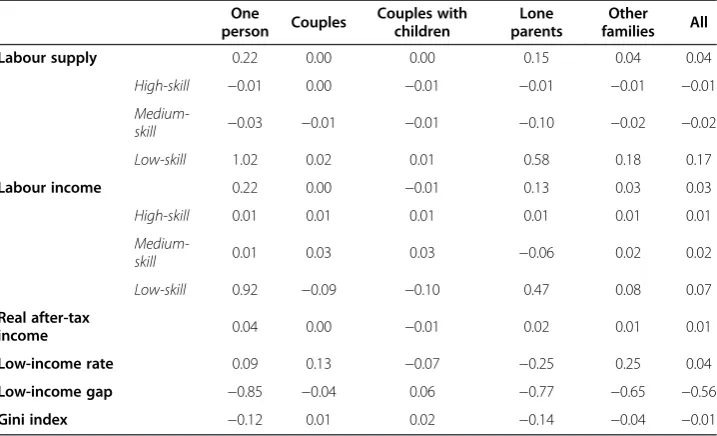
Table 7 Labour supply and distributional impacts of Scenario 3, % change from the base run
One
person Couples
Couples with children
Lone parents
Other families All
Labour supply 0.22 0.00 0.00 0.15 0.04 0.04
High-skill −0.01 0.00 −0.01 −0.01 −0.01 −0.01
Medium-skill −0.03 −0.01 −0.01 −0.10 −0.02 −0.02
Low-skill 1.02 0.02 0.01 0.58 0.18 0.17
Labour income 0.22 0.00 −0.01 0.13 0.03 0.03
High-skill 0.01 0.01 0.01 0.01 0.01 0.01
Medium-skill 0.01 0.03 0.03 −0.06 0.02 0.02
Low-skill 0.92 −0.09 −0.10 0.47 0.08 0.07
Real after-tax
income 0.04 0.00 −0.01 0.02 0.01 0.01
Low-income rate 0.09 0.13 −0.07 −0.25 0.25 0.04
Low-income gap −0.85 −0.04 0.06 −0.77 −0.65 −0.56
examining the impacts of the EITC and the WFTC. As stressed previously, lone parents and particularly women are those who benefit the most in terms of income and labour supply. However, the impacts are not comparable to the WITB since their characteris-tics differ.
As previously mentioned, the increase in labour supply would translate into income gains. The results show that the impacts are in line with the changes in work effort with Lone parents and One person households benefiting relatively more in terms of net-income under the three scenarios. The increase in after-tax income leads to a de-cline in the low-income rate and low-income gap. However, the changes in low-income rates are not only determined by the change in net income but also by the extent to which families belonging to the same group are clustered around the low income meas-ure (threshold). We also notice that the changes in the low-income rate are more pro-nounced for Couples and Couples with children. Regarding the impact on inequality, the Gini index declines for all household categories under Scenarios 1 and 2, and once again the magnitude is relatively higher for Lone parents. Conversely, the impacts on the low-income rates and inequality suggest that some households may be worse-off under Scenario 3. Nonetheless, the low-income gap declines among all family types ex-cept for couples with Children. In order to check whether these changes are statistically significant, we examine in the next section the robustness of low-income incidence and inequality comparison analysis.
5.3. Robustness analysis
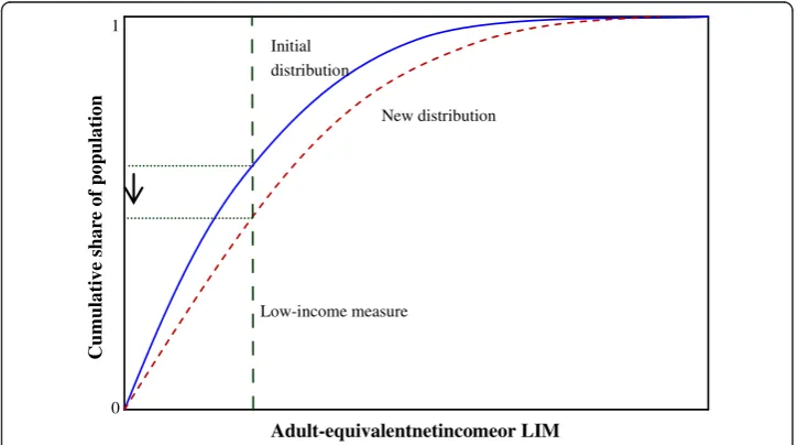
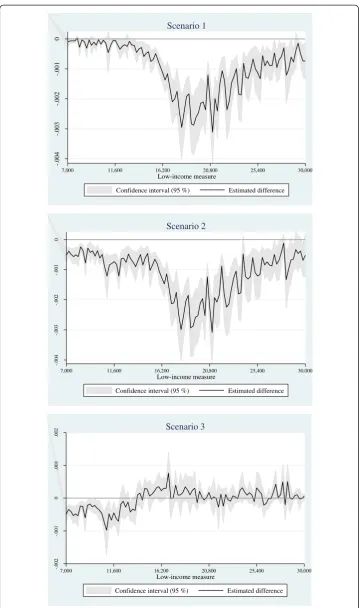
Given that low-income rates are sensitive to the choice of low-income measures (LIM), we examine in what follows the difference between cumulative distribution functions before and after the introduction of the WITB, often referred to as poverty dominance analysis. Poverty dominance analysis is based on the cumulative distribution function (also referred to as the FGT curve) which plots consumption or income on the horizon-tal axis and the cumulative share of the population on the vertical axis (Figure 5). If the
Low-income measure
New distribution Initial
distribution
C
u
m
u
la
ti
ve shar
e of popul
ati
o
n
1
Adult-equivalentnetincomeor LIM 0
-.
004
-.
003
-.
002
-.
001
0
20,800 16,200
11,600
7,000 25,400 30,000
Low-income measure
Confidence interval (95 %) Estimated difference
Scenario 1
-.
0
0
4
-.
0
0
3
-.
0
0
2
-.
0
0
1
0
7,000 11,600 16,200 20,800 25,400 30,000
Low-income measure
Confidence interval (95 %) Estimated difference
Scenario 2
-.
0
0
2
-.
0
0
1
0
.0
0
1
.0
0
2
7,000 11,600 16,200 20,800 25,400 30,000
Low-income measure
Confidence interval (95 %) Estimated difference
Scenario 3
-.0008
-.0006
-.0004
-.0002
0
11,600 16,200 20,800 25,400 30,000 7,000
Low-income measure
Confidence interval (95 %) Estimated difference Scenario 1
-.001
-.0008
-.0006
-.0004
-.0002
0
7,000 11,600 16,200 20,800 25,400 30,000
Low-income measure
Confidence interval (95 %) Estimated difference Scenario 2
-.0008
-.0006
-.0004
-.0002
0
7,000 11,600 16,200 20,800 25,400 30,000
Low-income measure
Confidence interval (95 %) Estimated difference Scenario 3
new distribution lies entirely to the right and below the initial distribution then we may assert with certainty that poverty has decreased regardless of where one draws the pov-erty line. If however the two povpov-erty incidence curves cross each other, we may look at the second or third order dominance using the FGT curves forα= 1 (low-income gap) andα= 2 (severity of low-income)33.
From Figure 6 and for a reasonable range of LIMs we may assert that the low-income rate declines under both Scenario 1 and 2 but the effects are more statistically significant under the latter for lower LIMs. However, we can assert that the decline is only significant for a narrow range of low LIMs under Scenario 3, as the results suggest that the two FGT curves cross each other at various levels. On the contrary, the robust-ness analysis of the changes in low-income gaps presented in Figure 7 implies that the shock leads to low-income gap alleviation wherever one draws the low-income measure.
Finally, dominance analysis may also be applied to inequality by computing the differ-ence between Lorenz curves (Figure 8). The Lorenz curve indicates the cumulative share of income held by a proportion p (percentile) of the population when households are sorted from lowest to highest income. This curve is increasing and convex since the new incomes that are being added when p increases are greater than those that have already been counted. If the difference between the initial and the new Lorenz curves is positive it indicates a decrease in inequality and vice-versa. Figure 9 confirms the above mentioned decrease in inequality among families of low-income earners and the likely opposite effect among some households as the Lorenz curves cross each other at some point. This implies that the change in inequality at the aggregate level under Scenario 3 is not robust to the choice of the inequality index.
0
1 Initial distribution New
distribution
C
u
m
u
la
ti
ve shar
e of i
ncom
e
1
Percentile
Line of perfect equality
0
.0
0
0
1
.0
0
0
2
.0
0
0
3
.0
0
0
4
.0
0
0
5
0 .2 .4 .6 .8 1
Percentile
Confidence interval (95 %) Estimated difference
Scenario 1
0
.0
0
0
2
.0
0
0
4
.0
0
0
6
0 .2 .4 .6 .8 1
Percentile
Confidence interval (95 %) Estimated difference
Scenario 2
-.
0
0
0
1
0
.0
0
0
1
.0
0
0
2
.0
0
0
3
.0
0
0
4
0 .2 .4 .6 .8 1
Percentile
Confidence interval (95 %) Estimated difference
Scenario 3
6. Conclusion
In 2007 the federal government introduced a new work incentive, the WITB, to en-courage individuals to enter the workforce and to reduce pressures on social programs. A number of studies that have examined the impact of such measures–in partial equi-librium framework – suggest that similar earning supplements are likely to have posi-tive effects on labour supply and poverty alleviation. In this study we have assessed the impact of this refundable tax credit in Canada, using an integrated microsimulation computable general equilibrium. The integrated approach employed enables a better assessment of the impact of policy shocks on labour supply and income distribution as it ensures that feedback effects, such as general equilibrium effects on wages, are fully captured in the simulations. To that end, we have estimated for the first time an Ex-tended Linear Expenditure System for 25 Canadian household categories. All estimated income elasticities are highly significant and consistent with the underlying theoretical model. In contrast, the Frisch parameter (defined as the negative value of the ratio of total consumption to discretionary consumption) provides a new insight about mini-mum consumptions which may be negative for some commodities deemed unneces-sary. For higher income families, however, minimum consumption is estimated to be around 20 percent.
Three scenarios were analysed taking into account increased work incentives for low-income earners, labour market participation of social assistance recipients, and the risk of higher marginal tax rates when the tax credit is phased out. At the aggregate level simulations results suggest modest positive impacts on labour supply and GDP, as well as a decline in low-income rates and income inequality. At the micro level, the WITB affect particularly labour market participation of low- and medium-skilled One person and Lone-parents families. These positive effects on labour supply translate into higher after-tax incomes leading to a decline in low-income rates and low-income gaps. Re-garding the impact on the Gini index, we find a decline in inequality across all house-hold categories especially lone parents. Finally, robustness analysis is performed showing that the declines in the low-income rate and inequality at the aggregate level are statistically significant only under Scenarios 1 and 2. Nevertheless, the results sug-gest that all three scenarios lead to an alleviation of the low-income gap wherever one draws the low-income measure. These findings suggest that enhancing the WITB could provide additional income support to working Canadian families while reducing work disincentives for those trapped behind the welfare wall34. The model developed in the current study could be used to examine the impact of different WITB designs (i.e., start of the benefit, phase-in and phase-out rates and ranges) on labour supply and income distribution.
Endnotes 1
Before April 2003, the Working Tax Credit (WTC) was merged with the Child Tax Credit as the Working Family Tax Credit (WFTC).
2
See Figure 2 for clarifications about the phase-in and the phase-out of earning supplements.
3
For a detailed discussion see Eissa and Liebman (1996) and Eissa and Hoynes (2005).
4
5
Previous initiatives in Canada included the self-sufficiency project which consisted in an earning supplement offered for a limited 3-year period to individuals who found full-time jobs and agreed to leave the income assistance program. For more informa-tion see Ford et al. (2003).
6
For a survey on applied microsimulation techniques see Davies (2009).
7
An Appendix with a complete list of equations is available from the authors.
8
Note that the present multisectoral CGE model may be used to analyse the impact of external shocks (e.g., decrease in world prices of manufacturing products or the in-crease in energy prices) on labour market and income distribution (See Annabi et al. 2013).
9
We consider the NOC skill levels 0 and A as high-skilled, level B as medium-skilled, and levels C and D as low-skilled workers.
10
This closure rule implies that all increases in income do not translate into only an increase in consumption but also stimulate saving and investment.
11
Note that with the closure rule discussed above, a scale parameter in the invest-ment demand function is endogenously adjusted to ensure that the savings-investinvest-ment identity is respected.
12
As in Annabi et al. (2008), Annabi et al. (2013), the current version of the model does not include a reweighting procedure reflecting future changes in household com-position. Blundell et al. (2013) suggest that welfare reforms may also change the returns to education and human capital accumulation. These aspects would increase consider-ably the complexity of the model and its numerical solution, and hence has been left for future research. See Davies (2009) for a detailed discussion on dynamic microsimulation.
13
The model is formulated as a system of nonlinear equations solved recursively as a con-strained non-linear system (CNS) with GAMS/Conopt3 solver and a 64bits operating system.
14
The general equilibrium assessment of a given policy requires using data prior to its implementation. In addition, only Annabi et al. 2013 data was final and available when the development of the first version of the model was initiated. A new version of the model calibrated to 2006 data is in progress. However, this would not affect the conclusions of the current study as the structure of the economy is expected to remain similar during such a short period.
15
A detailed description of the sectors and commodities included in the model may be found in Annabi et al. (2013).
16
Matching may be used in the opposite situation. In implementing their microsimu-lation CGE model to Russia, Rutherford and Tarr (2008) used this approach to estimate income sources for 55,098 households.
17
Aggregating households may be a useful strategy in explaining simulation results. However, one should keep in mind that each group may be very heterogeneous which prevents the link between the base-run characteristics and the aggregated results from being straightforward.
18
19
Income elasticities of demand have to be adjusted to respect Engel aggregation. Al-ternatively, one can use the price elasticities of demand. See Annabi (2003), Annabi et al. 2006 for details.
20
Studies about joint determination of labour supply and consumption are spread across countries and are very selective. See Green et al. (1978) for Canada, Blundell and Walker (1982) or Jorgenson and Slesnick (2008) for the US, and Asano (1997) for Japan.
21
See Blundell and MaCurdy (1999) for literature review. Most studies in this review focused on issues related to the intensive and extensive margins of work, while specific-ally controlling for gender, and other demographic or socioeconomic factors.
22
Models such as the Almost Ideal Demand System (Barnett and Seck 2006, Deaton and Muellbauer 1980), the Rotterdam model (Barten 1964), or the Translog model (Christensen et al. 1975, Srinivasan and Winer 1994) assume interior solutions and ig-nore the censoring of data. The Stone-Geary utility function is a better choice to cap-ture this behaviour.
23
We alsoconcentratedthe likelihood function, and reduced the number of parame-ters given that the variance covariance parameparame-ters are not our priority in this study (see Amemiya 1985 and Greene 1993).
24
The virtual price is the price the consumer is willing to pay for a given good and is always less than the actual price.
25
Standard errors were obtained using the delta method. See Appendix for a brief description of the econometric model.
26
EMTR have been generated with the MAPSIT model. For more details, see Morri-son (1990).
27
Contrary to the EITC, currently we do not have any information on the actual take-up rate of the WITB.
28
The current design of the WITB in Ontario does not include a plateau represent-ing the range for maximum benefits; See Chan et al. (2009) page 7.
29
Income distribution indices in the base run are presented in Table 8 in the Appendix.
30
In the absence of any complementary measure on the demand side, the increase in labour supply leads to a decline in real wages with respect to the benchmark equilibrium.
31
Low-income rate represents the share of households with income below the low-income measure, which is equal to fifty percent of median adjusted net low-income. Low-income gap is the amount of money by which each household’s income falls below the threshold. More details on income distribution indices are presented in the Appendix.
32
Distributional analysis is performed using DASP (Araar and Duclos 2009) and DAD (Duclos and Araar 2004).
33
For more details on poverty and inequality dominance analysis, see Duclos and Araar (2004), Araar et al. (2007), Bibi and Duclos (2009), and Chen and Duclos (2011).
34
Battle (2009) suggests that the WITB should gradually improve over time in order to become a major income support for working poor Canadians. On the other hand, Chan et al. (2009) recommend several modifications to the WITB in order to increase work incentives and to be more consistent with social programs in Ontario. To increase participation rates and full-time work, the authors suggest moving up the start of the credit, decreasing the phase-in rate, lowering the maximum benefit, and lastly changing the phase-out rate to remain cost-neutral with respect to the current program.
35
Appendix
Micro-econometric model
Let Ch= (Ch,1,…,Ch,m) be the consumption vector of mgoods by a household of typeh and P= (p1,…,pm) the corresponding price vector. Denote by Lh andwhthe leisure time and the wage rate, and letYF,hbe the full income35. The utility of each householdUh(Ch,Lh) takes the form of a Stone-Geary function and the corresponding optimisation problem is
maxCh;j; Lh;j Uh¼
Ym
j¼1
Ch;j−Chmin;j
αh;j
⋅ Lh−Lhmin
βh
s:t X m
j¼1
pjCh;jþwhLh≤YF;h ;
Xm
j¼1
αh;jþβh ¼1;j¼1;…;m;andh¼1;…;H
ð1Þ
where Cmin
h;j andLhminrepresent household’shminimum consumption of goodjand leis-ure time respectively. The parameters αh,jandβh represent marginal budget shares, and they should be strictly positive for at least some of the essential goods such as food or clothing. Estimates of model parameters are also used to derive income elasticities and the Frisch parameter (See Table 9). The total number of households is denoted byH. We also assume that the inter-group preferences are explicitly additive over Uh. Then the overall utility function will have the same form as in (1) with an additional product sign indexed from 1 toH. The analysis of all the groups can be simplified then to the analysis of a single group h. Without loss of generality, reorder the good vector so that the first
ℓ≥0 elements correspond to zero consumption, i.e.,Ch= (0,…, 0,Ch,ℓ+ 1,…,Ch,m), and the remaining goods are indexed 1 + 1 through m. Include leisure time in the consumption vector and let P= (p1,…,pj−1,wh,pj+ 1,…,pm) be the corresponding vector price. The Kuhn-Tucker (KT) conditions for the consumption of goods are:
αh;j Ch;j−Chmin;j
−λpj≤0 for j¼1;…;ℓ
αh;j Ch;j−Chmin;j
−λpj¼0 for j¼ℓþ1;…;m
ð2Þ
and for labour supply:
βh Lh−Lhmin
−λwh≤0 if Lh¼0
βh Lh−Lhmin
−λwh¼0 if Lh>0
ð3Þ
The corresponding interior solutions defining the Extended Linear System (ELES) are
pjCh;j¼pjChmin;j þ
αh;j 1−βh
Xm
i¼1
piCh;i−
Xm
i¼1
piChmin;i !
LSh¼Maxhourh− 1 wh
βh 1−βh
Xm
i¼1
piCh;i−
Xm
i¼1
piChmin;i ! 8 > > > > < > > > > :
ð4Þ
where LSh−Maxhourh ¼− Lh−Lhmin
sh;j¼ pjCh;j
Xm
i¼1
piCh;i
; j¼1;…;m;andi¼1;…;m ð5Þ
The KT solutions can equivalently be expressed in terms of virtual prices (Neary and Roberts, 1980). The virtual prices for the non-consumed goods and leisure are the prices the consumer is willing to pay for a given good or leisure and are always lower than actual prices, defined as:
ξj¼
dUh dCh;j=λ
¼ αh;j
Ch;j−Chmin;j
=λ≤pj
ξL¼
dUh dLh =λ
¼− βh
LSh−Maxhourh
ð Þ=λ≤wh
ξj≤pjandξL≤wh for j¼1;…;ℓ andξj¼pj for j¼ℓþ1;…;m
ð6Þ
Using (3) and the virtual prices and wage in (6) we obtain:
pm dUh dCh;j−ξj
dUh dCh;m−
¼0 ; j¼1;…;m
pm dUh
dLh −ξL dUh dCh;m
¼0
ð7Þ
The non-negativity constraint on the parametersαis imposed by the following form:
αh;j¼eεh;j ð8Þ
where εh(εh,1,εh,2,…,εh,m) are error terms and are normally distributed with means γh (γh,1,γh,2,…,γh,m) and a constant variance-covariance matrix ∑. We apply the
normalisation εh,m= 0 and preserve the condition
Xm
j¼1
αh;jþβh ¼1 in (1) using the
fol-lowing parameterisation:
θh;j¼Xn αh;j
j¼1
αh;jþβh
;forj¼1;…mandθβh¼
βh
Xn
j¼1
αh;jþβh
ð9Þ
Using (4), (5), and (6) we define the following expression of the virtual prices for non-consumed goods and the virtual wage:
ξh;j¼pj
sh;m−pmChmin;m=Yh sh;j−pjChmin;j =Yh
eεj ð10Þ
ξh;L¼−wh
sh;m−pmChmin;m=Yh sL−whMaxhours=Yh
eεh;L ð11Þ
where Yh¼
Xm
i¼1
piCh;i and sL¼whYLShh. After logarithmic transformations of the virtual
εh;j≤ln − pjChmin;j
Yh !
−ln sh;m−
pjCmin
h;m
Yh !
; j¼1;…;m
εh;j¼ ln sh;j− pjChmin;j
Yh !
−ln sh;m−
pjCmin
h;m
Yh !
;j¼lþ1;…;m
εh;L¼ ln
wMaxhours Yh
−ln sh;m−
pjChmin;m Yh
!
forLSh ¼0
εh;L¼ ln −
sL−wMaxhours Yh
−ln sh;m−
pjChmin;m Yh
!
forLSh >0
g ð12Þ
The error terms are defined as follows:
e1;h ¼ εh;1−γh;1;…;εh;l−γh;l
T
e2;h¼ εh;ℓþ1−γh;ℓþ1;…;εh;m−1−γh;m−1
T ð13Þ
and the shares of the consumption goods are defined ass2,h= (sh,ℓ+ 1,…,sh,m−1).
The likelihood contribution function of a householdhfor an observationxi,hin each of consumption regimek(positive or null) is:
Lh;k xi;h ¼ ∫η: η≤rf ηh dηh
f e2;h
∂e2;h
∂s2;h
ð14Þ
where the Jacobian of the transformation (see Kao et al. 2001) is given by:
∂e2;h
∂s2;h
¼ Xm
i¼ℓþ1
si;h−piChmin;i
=Ym
i¼ℓþ1
si;h−piChmin;i
ð15Þ
The likelihood withnobservations is:
Lh¼
Yn
i¼1
∏
k Lh;k xi;h
Iið Þk
ð16Þ
whereIi(k) indicates to what regime the households is switching and takes the value of
Ii(k) = 1, if the observation consumption patternxi,hfor an individuali in the category of householdhis in the demand regimek, andIi(k) = 0 otherwise.
Since var ηh ¼Ωh≡Σ11h−Σ12;hΣ−221;hΣ21;h for the ELES from (14) is positive defin-ite, there exists a lower diagonal Choleski matrix with positive diagonal elements such that AA’=Ωh. Define a transformation ζh=A−1ηh. The transformed random variable ζh becomes a standard multivariate normal variable. The likelihood func-tion in (14)becomes:
Lh;k xi;h ¼ ∫fζh:Aζh≤rhg
Yℓ
i¼1
ϕ ζi;h
" #
dζh !
f e2;h
∂e2;h
∂s2;h
ð17Þ
where ϕ(ζh,i) is the standard normal density of ζh,i,ζh= (ζh,1,…,ζh,ℓ). The bounds
∫a−−111∞r1∫a −1
22ðr2−a21ð Þζ1;h Þ
−∞ …∫a
−1
llðrl−al1ζh;1−al2ζh;2−…−al;l−1ζh;l−1Þ
−∞ Y
l
i¼1
f ζh;i
!
dζh;1…dζh;l
" #
f2 e2;h
∂e2;h
∂s2;h
ð18Þ
Now, transform the domain of integration to the unit interval of dimension1 by
de-fining the truncated standard normal density asφDið Þ ¼ζh φ ζh
ð Þ
Φð Þai ; where
ai¼a−ll1 rl−al1ζh;1−al2ζh;2−…−al;l−1ζh;l−1
with i= 1,K…, 1 and the domain Di= (–∞,ai] as a support of the density function. The likelihood function becomes:
Lh;k xi;h ¼ ∫
D1
…∫
Dℓ
Yℓ
i¼1
Φð Þai !
Yℓ
i¼1
ϕ ζh;i
dζh;1…dζh;l !
f2 e2;h
∂e2;h
∂s2;h
ð19Þ
Transforming the truncated normal random variables into uniform random variables
ui;h ¼
Φ ζð Þi;h
Φð Þai withξi,h≤aifori= 1, K…, 1; whereξi,his the virtual price of goodi. Condi-tional onζh,1,…,ζh,i−1,generate the uniform random variableui,hon [0, 1], through the inverse distribution transformation of ζi,h. This transformation defines a sequence of conditional uniform random variables. Once ui,h are drawn from a uniform random generator, ζ’s can be found recursively as functions of the drawn u’s ζi,h=Φ−1[ui,
hΦ(ai)] with the starting value as ζ1;h¼Φ−1 u1;hΦ ar111
h i
. This transformation allows changing the bounds of the integral into zero–one limits. With the realisation ofR ran-dom draws, the likelihood at a sample observationxnobx,hcan be simulated as:
Lh;k xnobs;h
¼ 1 R XR j¼1 Yℓ i¼1
Φ a−ll1 rl−al1ζh;1−al2ζh;2−…−al;l−1ζh;l−1
" #
f2 e2;h
∂e2;h
∂s2;h
ð20Þ
where nobs= 1,…..,Nobsis the index for the number of observations, andNobs is the total number of observations.
The total likelihood function for all the observations for the householdhis:
Lhð Þ ¼xh
Y Nobs nobs¼1 1 R XR j¼1 Yℓ i¼1
Φ a−ll1 rl−al1ζh;1−al2ζh;2−…−al;l−1ζh;l−1
" #
f2 e2;h
∂e2;h
∂s2;h
ð21Þ
fornobs= 1,…,Nobs.
Low-income and inequality indices
FGTα¼XN 1
i¼1
wini
⋅ XH
i¼1
wini z−yi
z
α
; i¼1;2;…;H;…;N
Where
N: Total number of households
H: Number of households whose income lies below the low-income threshold ni: Household size
wi: Sample weights
z: Low-income threshold
yi: Adult-equivalent after-tax income
The higher the value of α, the greater the weight given to low-income house-holds. When α= 0 the index FGT0 measures the low-income rate, also known as
the headcount ratio, which is equal to the ratio of the number of households (individuals) below the low-income measure to the total population. If α= 1 we obtain the low-income gap (depth) which measures the amount of money (in proportion of the low-income measure) by which each household falls below the threshold. One can also compute the severity of poverty assuming α= 2. In this case more weight is given to the lowest income and hence to the largest income gaps.
Regarding inequality, the most common measure is based on the Gini index which can be computed using different methods. Geometrically the value of the index can be calculated using the Lorenz curve (Figure 8). This curve shows the cumulative share of income held by a given proportion of the population. The value of Gini is equal to the ratio of the area between Lorenz curve and the perfect equality line to the area below this line (diagonal). Gini index ranges between 0, where each member of the population earns the same amount of income, and 1 where all income is held by only one member. The simplest numerical approach for computing the gini index is based on the relative deprivation method which does not require ranking observation by increasing order of
Table 8 Income composition (Million dollars) and distribution by family type in the base run
One
person Couples
Couples with children
Lone parents
Other families All Labour
income 60542 117605 258545 22741 101165 560598
High-skill 22915 43307 90757 5967 28531 191477
Medium-skill 23657 45141 104549 9245 41146 223738
Low-skill 13970 29157 63239 7529 31489 145384
After-tax
income 98830 174917 267456 33387 131911 708504
Low-income
rate 0.28 0.07 0.04 0.24 0.12 0.10
Low-income
gap 0.10 0.02 0.01 0.07 0.04 0.03
Table 9 Income elasticities of demand and Frisch parameters by household category
Less than $15,000 $15,000 to $35,000 $35,000 to $55,000 $55,000 to $100,000 $100,000 to 150,000
OP CO CC LP OT OP CO CC LP OT OP CO CC LP OT OP CO CC LP OT OP CO CC LP OT
Number of observations
1053 128 20 136 542 2169 1537 1026 1015 1365 777 2094 2686 507 1467 265 1476 3336 254 958 13 226 639 12 193
Agriculture and forestry
0.11 0.19 - 0.09 0.14 4.86 3.24 2.54 0.17 3.73 6.34 3.45 3.70 4.25 4.83 10.14 4.64 3.40 3.76 5.70 - 3.45 8.76 - 8.89
(0.00) (0.03) - (0.02) (0.01) (0.01) (0.01) (0.01) (0.01) (0.01) (0.03) (0.01) (0.01) (0.01) (0.01) (0.07) (0.01) (0.01) (0.04) (0.04) - (0.01) (0.05) - (0.07)
Other mining 4.96 2.00 - 6.67 9.76 5.20 6.11 3.65 7.29 4.41 15.45 5.58 9.25 12.51 5.54 12.20 7.31 6.11 7.30 13.10 - 5.58 14.50 - 14.30
(0.03) (0.24) - (0.58) (0.39) (0.05) (0.02) (0.02) (0.19) (0.07) (0.33) (0.03) (0.04) (0.10) (0.02) (0.35) (0.06) (0.02) (0.11) (0.15) - (0.03) (0.16) - (0.11)
Food, drink and tobacco
0.10 0.20 - 0.00 0.00 0.79 0.59 0.60 0.17 0.65 1.17 0.85 0.88 0.93 1.16 1.22 1.18 0.92 1.03 1.16 - 0.85 1.97 - 1.75
(0.00) (0.03) - (0.00) (0.00) (0.00) (0.00) (0.00) (0.01) (0.00) (0.01) (0.00) (0.00) (0.00) (0.00) (0.01) (0.00) (0.00) (0.01) (0.01) - (0.00) (0.01) - (0.01)
Textiles and clothing 6.62 0.30 - 3.95 4.80 5.94 2.06 3.16 0.15 6.90 1.81 2.07 1.77 0.51 1.67 2.33 2.03 2.00 1.91 1.95 - 2.07 1.03 - 1.29
(0.02) (0.04) - (0.44) (0.31) (0.05) (0.01) (0.01) (0.01) (0.06) (0.03) (0.01) (0.01) (0.00) (0.01) (0.06) (0.02) (0.01) (0.03) (0.02) - (0.01) (0.01) - (0.02)
Lumber and wood 10.54 17.48 - 0.07 0.11 2.50 20.23 3.05 0.11 4.45 14.43 7.31 4.38 13.02 11.93 9.89 7.14 9.03 8.95 5.59 - 7.31 4.39 - 10.09
(0.26) (1.12) - (0.01) (0.01) (0.05) (0.58) (0.06) (0.00) (0.12) (0.63) (0.18) (0.09) (0.37) (0.35) (1.01) (0.24) (0.15) (0.66) (0.18) - (0.18) (0.22) - (0.57)
Refined and other petroleum products
7.30 0.00 - 7.12 4.62 2.40 0.58 1.79 6.23 2.24 1.22 2.08 2.34 2.30 0.96 2.33 2.96 2.61 2.98 2.71 - 2.08 1.62 - 1.66
(0.14) (0.00) - (0.32) (0.24) (0.03) (0.00) (0.01) (0.10) (0.04) (0.02) (0.01) (0.01) (0.02) (0.00) (0.07) (0.02) (0.01) (0.07) (0.03) - (0.01) (0.01) - (0.02)
Machinery, motor vehicles and parts
34.75 20.91 - 33.82 1.07 4.86 5.49 6.44 16.23 5.95 2.10 1.31 4.13 1.73 2.19 0.89 0.56 0.81 0.73 1.30 - 1.31 1.12 - 1.26
(5.91) (1.19) - (12.09) (0.05) (0.35) (0.41) (0.54) (1.29) (0.57) (0.13) (0.06) (0.16) (0.14) (0.11) (0.05) (0.02) (0.02) (0.05) (0.04) - (0.06) (0.04) - (0.08)
Other manufactures 0.30 0.18 - 0.10 0.13 1.24 1.16 1.18 0.16 1.25 1.19 1.61 0.77 1.54 0.71 0.96 1.95 1.69 1.71 0.80 - 1.61 1.43 - 1.24
(0.00) (0.02) - (0.02) (0.01) (0.01) (0.00) (0.00) (0.01) (0.01) (0.01) (0.01) (0.00) (0.00) (0.00) (0.01) (0.01) (0.00) (0.02) (0.01) - (0.01) (0.01) - (0.02)
Utilities 1.23 2.57 - 2.43 3.94 1.41 0.58 0.99 2.01 1.16 3.98 3.40 2.74 1.85 3.10 4.84 4.45 3.76 4.44 3.88 - 3.40 3.29 - 3.08
(0.01) (0.24) - (0.20) (0.14) (0.01) (0.00) (0.01) (0.05) (0.02) (0.08) (0.02) (0.01) (0.01) (0.02) (0.14) (0.04) (0.02) (0.07) (0.04) - (0.06) (0.05) - (0.24)
2.93 12.72 - 8.19 6.18 2.38 2.86 3.36 6.57 2.66 1.35 2.21 2.84 2.74 1.53 5.16 2.14 2.66 2.38 2.87 - 2.21 1.69 - 2.30
al.
IZA
Journal
of
Labor
Policy
Page
29
of
33