Tracking Time Evolving Data Streams for Short-Term Traffic
Forecasting
Amr Abdullatif1•Francesco Masulli1,2• Stefano Rovetta1
Received: 12 June 2017 / Revised: 1 October 2017 / Accepted: 2 October 2017 / Published online: 24 October 2017 The Author(s) 2017. This article is an open access publication
Abstract Data streams have arisen as a relevant topic during the last few years as an efficient method for extracting knowledge from big data. In the robust layered ensemble model (RLEM) proposed in this paper for short-term traffic flow forecasting, incoming traffic flow data of all connected road links are organized in chunks corre-sponding to an optimal time lag. The RLEM model is composed of two layers. In the first layer, we cluster the
chunks by using the Graded Possibilisticc-Means method.
The second layer is made up by an ensemble of forecasters, each of them trained for short-term traffic flow forecasting on the chunks belonging to a specific cluster. In the oper-ational phase, as a new chunk of traffic flow data presented as input to the RLEM, its memberships to all clusters are evaluated, and if it is not recognized as an outlier, the outputs of all forecasters are combined in an ensemble, obtaining in this a way a forecasting of traffic flow for a short-term time horizon. The proposed RLEM model is evaluated on a synthetic data set, on a traffic flow data simulator and on two real-world traffic flow data sets. The model gives an accurate forecasting of the traffic flow rates with outlier detection and shows a good adaptation to non-stationary traffic regimes. Given its characteristics of out-lier detection, accuracy, and robustness, RLEM can be fruitfully integrated in traffic flow management systems.
Keywords Traffic forecastingFuzzy clusteringBig
dataEnsemble modelEvolving data streams
1 Introduction
Data streams are ordered, potentially unbounded sequences of observations (data elements) made available over time
[24, 43, 57, 58]. Data stream mining, the process of
extracting knowledge from them, has arisen as a relevant topic in the machine learning field during the past decade [3].
In many data stream mining applications where data exhibit a time series nature, the goal is to predict infor-mation about future instances in the data stream given some knowledge about previous ones. This can be approached either by modelling of the dynamics of the system, or by autoregressive models. Within the field of road traffic analysis and forecasting, the latter approach has
rapidly become widespread in recent years [48] due to the
increase in both availability of sensed data and processing power to deal with them.
A common requirement in the task of mining data streams is the ability to distinguish the useful information from the useless ones. This may be required for limiting the usage of resources, for instance transmission bandwidth or storage memory; for summarization purposes; or even for relieving the user from information overload. As an example of this latter case, a sensor network may provide just the information that requires attention by the human supervisor, rather than transmitting all records. This task
goes by the name of anomaly or outlier detection [7,11].
One common approach to anomaly detection makes use of unsupervised learning: we learn a baseline model of the phenomenon of interest, and then measure the discrepancy
& Amr Abdullatif
1 DIBRIS - Department of Informatics, Bioengineering,
Robotics and Systems Engineering, University of Genoa, Via Dodecaneso 35, 16146 Genoa, Italy
2 Sbarro Institute for Cancer Research and Molecular
Medicine, Center for Biotechnology, Temple University, Philadelphia, PA, USA
of subsequent data from the baseline. An anomalous observation is the one that is not well explained by the model.
When operating within non-stationary environments for an extended time, the source of the stream may change over time. We distinguish between two types of change: for
evolutionary, smooth changes, we use the term concept
drift, while a radical, sudden change is labelled concept shift.
In this paper, we approach the problem of short-term
traffic forecasting by employing the autoregressive
approach, more suitable than a model-based one in the short-term because it can exploit the local time informa-tion, contained in recent observations and is computation-ally less demanding.
To tackle the issues of anomalies and non-stationarity, we employ an extension of the possibilistic clustering
approach [34, 35] named Graded Possibilistic c-Means
[15,38] as a means to perform clustering of the
non-sta-tionary streaming data and employ the knowledge accu-mulated into the clusters to build a robust, accurate short-term traffic forecaster. Our proposed method has the ability to prevent outliers in the data stream from having a strong effect on the forecasting accuracy and is capable of both learning the data stream and analysing its evolution for the purpose of tracking it. To this end, an index to measure data stream change is proposed, based solely on the memberships to clusters, and not on additional measures.
We focus on the online approach to track and adapt to concept drift and shift and on using this knowledge to improve the ensemble forecasting model that was proposed
in [1] by making the model able to not only detect outliers,
but also track the changes in data streams.
An incremental retraining strategy is adopted, where the amount of retraining, and therefore the required computa-tional effort, is modulated by the proposed measure of model change.
This paper is organized as follows. The next section summarizes the state of the art in streaming data clustering and traffic modelling, motivating the specific design
choi-ces of our proposal. Section3 describes the proposed
methodology. Section4.1 presents the experimental
vali-dation and the discussion of results. Conclusions are given in Sect.5.
2 Previous Work in the Fields of Data Stream
Mining and Short-Term Traffic Forecasting
The subject of this work is traffic forecasting. This is one of the most relevant problems related to data stream mining. It can be cast either in the long term, where forecasts are used to configure and validate road management plans, or in the
short term, for real-time decision-making. Short-term forecasting is the subject of this work.
Forecasting can be done with a system identification
approach, often with macroscopic models [22]. Although it
gives the most reliable results in the long-term forecasting problem, this approach is often not feasible for short-term forecasting, due to the inherent complexity of an accurate, first-principles model. The computation time required is often not compatible with the response time required.
The usual practice in this case is to use methods that forecast based on observations. This approach has devel-oped out of the growing availability of data and, in parallel, of methods from data science, machine learning and
computational intelligence [48].
Methods presented in the recent literature can be
cate-gorized into parametric models [16,21, 46] and
nonpara-metric or hybrid models [44,47,56].
Many traffic forecasting approaches focus on the prob-lem of freeway/motorway traffic forecasting in which the state of the road traffic is quite stable. In contrast, traffic forecasting in urban and network-scale areas is more complex because of the rapid change of traffic behaviour and of the limited availability of sensors that can cover the whole network.
Many approaches based on nonparametric models to tackle this problem have been proposed, such as multilayer perceptron with a learning rule based on a Kalman filter
[49], wavelet-based neural network [18], fuzzy-neural
model [52], ARIMA models [23], graphical-lasso neural
network [20], multi-task neural network [19], multi-task
ensemble neural network [45], k-nearest neighbour
non-parametric regression [53].
Most of these approaches are not meant to track changes
in traffic behaviour [48]. This is the main motivation for
our proposal, which is described in the next section. Since our method is centred around data stream clus-tering, we also survey some related work on this topic.
Most algorithms in this area [2, 4, 5, 26] focus on two
aspects: detecting outliers without taking concept drift tracking into consideration and clustering irregularly dis-tributed data, which is a challenging direction of research in the field.
Data stream clustering methods can be of the batch type, collecting a number of instances and then performing
clustering on these accumulated data [31, 40]. Other
methods are single-pass, storing summaries of past data as
they are scanned [25]. The strategies of these algorithms
can be incremental [9] or divide-and-conquer [4]. Yet other
algorithms alter the structure of the data themselves so that
they can be more effectively accessed [55].
Some popular stream clustering methods are density-based: they aim to find clusters of arbitrary shape by
modelling them as dense regions separated by sparse regions [6,13].
While this class of algorithms is popular and effective, they all produce only crisp partitions with no direct way to evaluate the outlierness of incoming data. An alternative strategy is to use fuzzy modelling for clustering.
Several incremental fuzzy clustering algorithms based
on fuzzy c-means (FCM) [8] to track non-stationarity in
data streams have been developed. Under the fuzzy mod-elling paradigm, each data point belongs to a cluster to a degree specified by a membership value. In general, as no membership is exactly null, a data point belongs to all clusters with different degrees.
Popular incremental fuzzy clustering algorithms for data
streams include single-pass FCM [27] and online FCM
(OFCM) [28]. Both process data chunk by chunk
(by-pat-tern) and estimate centroids for entire data set by extracting summary information from each chunk, but the ways they handle chunks are different.
In [36], two algorithms based on fuzzy c-medoids
(FCMD) [33], called online fuzzyc-medoids (OFCM) and
history-based online fuzzy c-medoids (HOFCMD), are
developed for clustering large relational data sets. In [39],
it is shown that one medoid may not be sufficient to capture
the underlying structure of a cluster. As a solution, in [50]
an incremental fuzzy clustering approach called incre-mental multiple medoids-based fuzzy clustering (IMMFC) was proposed, which is based on the idea of OFCM and HOFCMD and includes a mechanism to select multiple medoids instead of a single one to represent each of the clusters in each chunk.
3 Methodology
Our choice has fallen on an autoregressive approach which forecasts one step in future after observing a suitable in-terval of past observations.
3.1 Data Pre-processing
The observed data are samples of traffic flow on a road network. At any given time, each arc of the network graph contains a given number of vehicles. Flow is defined as the number of vehicles per unit time. An arc is characterized
by a maximum number of vehicles, itscapacity. When flow
approaches this value, the traffic slows down and enters a stop-and-go regime. Once the capacity is reached, traffic is entirely congested. We will be mainly concerned with relative flow, the ratio of flow to the arc capacity. Flow is sampled at discrete time intervals of the order of some minutes.
As already mentioned, data are organized in chunksof
observations corresponding to a time lag vector. To fore-castfta, the traffic flow on arcaat timet, a vector of length
T(the lag period) is used to represent a given chunk: x¼ftaT;ftaTþ1;. . .;fta1: ð1Þ
The vector x thus obtained describes the pattern of
traffic flow variation over one past time interval of duration
Tin a neighbourhood of sizen of arca. In the rest of this
paper, x will be the input to the method that is being
described.
3.2 Forecasting Model Issues
The design of autoregressive methods requires solving the following issues.
Lag PeriodProper selection of the lag periodT, the size of the chunks, is crucial because it affects the correct representation of the data stream source. If the lag period is chosen too small, then we will not be able to distinguish
between the time lag vectors in the vector space [10];
hence, the prediction process will be practically impossible because data do not carry enough valuable information. If the lag period is chosen too large, measurement will refer to times which are too far to have a significant correlation with the present, and therefore they will be irrelevant and act as noise [30].
In this paper, we adopt the minimum of the time-delayed
mutual information as an estimation of the time lag [17]:
SðsÞ ¼ X
ij
pijðsÞln
pijðsÞ
pipj ð2Þ
where for some partition of the real line into intervals:
• piis the probability to find a time series value in theith
interval,
• pijðsÞis the joint probability that an observation at any
timet falls into the ith interval and the observation at
timetþsfalls into thejth one.
Unlike the autocorrelation function, the mutual infor-mation takes into account also nonlinear correlations. If the time-delayed mutual information exhibits a marked
mini-mum, then T¼arg minsSðsÞ is a good candidate for a
suitable time delay. The obtained values are then confirmed by checking them against domain knowledge.
Note that if the minimum is not sufficiently prominent, then another method should be used. In the case of road traffic, the ‘‘memory’’ of the system is limited and this problem did not occur in our experiments.
Training Set Size This refers to the number of obser-vation patterns that will be used to train the forecasters. This is usually not under the control of the designer, but in
the problem at hand the availability of data has been found to be sufficient.
Outliers Handling Learning patterns with a different behaviour using the same model tends to reduce the model’s performance. This can occur for both diversity in the operating conditions, in the presence of a stationary source, and changes in the underlying source itself (concept drift and shift), in the non-stationary case.
Accordingly, the proposed model focuses on two strategies: learning an ensemble of locally specialized models and explicitly measuring outlierness.
3.3 Robust Layered Ensemble Model
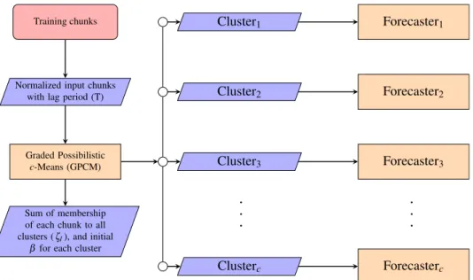
The proposedrobust layered ensemble model(RLEM) for
short-term traffic forecasting consists of two layers as
shown in Fig.1 and is able to track the changes in data
streams, such as traffic flows, and to use this information to improve the forecasting accuracy.
The first layer of RLEM consists in a fuzzy clustering process having as its goals to cluster traffic flow chunks
intocfuzzy clusters, where chunks with high membership
to the same cluster represent similar temporal patterns, and at the same time to measure the outlierness degree of each chunk and consequently to measure the density of outliers. To this aim, we employ an incremental clustering
pro-cess based on the Graded Possibilisticc-Means (GPCM)
[38] that is able to adapt to the changes in the traffic flow,
by implementing a continuous learning that exploits the input chunks as they arrive. Intrinsic to this clustering method is a measure of outlierness that provides informa-tion about the goodness of fit of each input chunk to the clustering model.
In the second layer, an ensemble of a number of base
learners acting as forecasters equal to the number c of
clusters is used, each of them specialized on a homoge-neous region of the data space. This approach follows the
mixture of local expertsmodel proposed in [29].
To obtain thechomogeneous regions of the data space
needed for base learner training, we defuzzify the fuzzy segmentation performed by the first layer by assigning each chunk to the cluster where it has the highest membership (nearest neighbour criterion). To implement the base forecasters, we employ time-delayed neural networks
(TDNN) [14] trained with the error back-propagation
algorithm. Other choices may be implemented as well. The TDNN model is simply a multilayer perceptron neural network whose input is a time lag vector. In this work, one-hidden-layer networks are used for this purpose. We will indicate the network topology by specifying just the number of input, hidden and output units as a triplet, ni-nh-no, with the understanding that each layer is fully
connected to the following and that hidden units are sig-moidal while output units are linear.
The measure of outlierness evaluated by the first layer is used in the second layer to assess and improve the fore-casting accuracy.
In the following, we describe the specific clustering technique used.
3.4 The Graded Possibilisticc-Means
In central clustering, we have a training set ofninstances
(random vectors) and c clusters represented by means of
theircentralpoints or centroidsyj. Many central clustering
methods perform the minimization of a objective function
[8], that usually is the expectation of the distortion:
D¼1 n Xn l¼1 Xc j¼1 uljdlj; ð3Þ l¼1;. . .;n; j¼1;. . .;c; dlj¼ kxlyjk 2 ð4Þ
optimized with respect to centroidsyjand membershipsulj,
with some constraints placed on the total mass of
mem-bership to clusters
fl
Xc
j¼1
ulj: ð5Þ
In Eqs.3and5,nis the cardinality of the data set,cis
the number of clusters, while fl can be interpreted as the
total membership mass of observationxl. In the following
of this subsection, we outline some relevant fuzzy central cluster models.
The first model we present is the maximum entropy
(ME) or deterministic annealing approach [42] that
impo-ses fl¼1. In this case, we are in the probabilistic case,
where memberships are formally equivalent to
probabilities.
In addition to the expectation of the distortion (Eq.3),
the objective functionJMEof ME includes the probabilistic
constraint. The necessary conditions for the minimum of
JMEare rJME¼0 that yields:
ulj¼ edlj=b fl ð6Þ and yj¼ Pn l¼1uljxl Pn l¼1ulj : ð7Þ
Equations6 and7 can be interpreted as the basis of a
at different levels of temperature (or fuzziness) that is
regulated by the value of b (deterministic annealing
pro-cedure). Whenbis large, the free energy is equivalent to
the unconstrained optimization of the expectation of the
distortion (Eq.3).
The objective function of ME is formally equivalent to
the one of fuzzyc-means [8], and both of them show the
problem of low outlier rejection: The memberships of outliers can be very large, not different from those of inliers.
In contrast to ME, the possibilisticc-means (PCM) [35]
does not impose any constraint onfl, so memberships are
not formally equivalent to probabilities but represent degrees of typicality to clusters.
The objective of PCM, JPCM includes an individual
parameterbj for each cluster, andrJPCM¼0 yields
ulj¼edlj=bj ð8Þ
for membership of instances to clusters and Eq.7 for
cluster centres. Again, Eqs.7 and8 can be interpreted as
the basis of a Picard iteration for the minimization ofJPCM.
As discussed in [35], while the PCM produces
mem-bership functions that can be interpreted as measures of typicality of instances to clusters and shows a strong outlier rejection, the Picard iterations may fail to converge due to
the lack of competitive terms in Eq.8.
The graded possibilistic c-means (GPCM) clustering
model proposed by our group [38] exploits the similarities
of Eqs.6 and8 to obtain both the nice properties of
memberships with the meaning of typicality and strong outlier rejection of the PCM and the convergence ability of the ME.
In this paper, we present a new simpler version of the GPCM. To this aim, we propose the following formula that
unifies the Eqs. 6and8:
ulj¼ vlj Zl ; ð9Þ where vljedlj=bj ð10Þ
is called the free membership and Zl is the generalized
partition function that is a function of the membership massfl.
This allows us to add a continuum of other, intermediate cases to the two limit case models just described,
respec-tively, characterized by Zl¼fj (probabilistic) and Zl¼1
(possibilistic). Here, we use the following formulation:
Zlfal ¼ Xc j¼1 vlj !a ; a2 ½0;1; ð11Þ
where the parameteracontrols thepossibility level, from a
totally probabilistic (a¼1) to a totally possibilistic (a¼0)
model, with all intermediate cases for 0\a\1. The Picard
iteration implementing the GPCM iterates the membership
evaluation (Eq. 9), and the cluster centres evaluation
(Eq. 7) until convergence.
In the GPCM model at each iteration of the Picard
procedure,bj is updated [35] according to:
bj¼
PN
i¼1uijdij
kPNi¼1uij
; j¼1;. . .;c ð12Þ
Note that in the GPCM after trainingfl2 ð0;cÞdepends
on the value of a. More specifically:
Fig. 1 Diagram of the training stage in the RLEM. See text for details on the quantities and on the operational blocks mentioned in the diagram
• values fl1 are typical of regions well covered by
centroids;
• but fl1 is very unlikely for good clustering
solutions, since it implies many overlapping clusters;
• finally, fl1 characterizes regions not covered by
centroids, and any observation occurring there is an outlier.
In order to reject outliers, let us define the degree of
outliernessindexX, corresponding to the concept ofbeing an outlier, as follows:
XðxlÞ ¼max 1f fl;0g: ð13Þ
For each threshold onX we set, we obtain a region of
inlier in the data space and we define as outliers the data outside this region.
Differently from other approaches based on analysing
instance-centroid distances [54], the GPCM provides a
direct measure of outlierness that is not referred to local density or to individual clusters, but is defined with respect to a whole clustering model.
Outlierness can be modulated by an appropriate choice
of a. Low values correspond to sharper outlier rejection,
while higher values imply wider cluster regions and
therefore lower rejection. Fora¼1, the GPCM becomes
probabilistic and loses its ability to identify or reject outliers.
We can define the initialoutlier density q02 ½0;1Þ as
theaverage degree of outlierness: q0¼ 1 jW0j X l2W0 XðxlÞ; ð14Þ
where W0 is an initial window of data to ‘‘bootstrap’’
GPCM and provides an initial clustering.
The average densityq0accounts for both frequency and
intensity, or degree of anomaly, of outliers. This is a mean, so quantity and intensity can compensate each other, so that the effect of few strong outliers is the same as that of many moderate outliers.
During execution, outlier intensity at step l[jW0j is
computed as follows:
ql¼0:01Xðxl1Þ þ0:99ql1; ð15Þ
whereXl is the measure of outlierness at stepl. Note that
the density is a function of the past values, being a convex combination of current outlierness and past density (ex-ponentially weighted moving average). The exponential
time constant is ln 1004:6, similar to the typical lag
periodsTused in this study.
The updating formula can also be rewritten as
ql¼ql1 þ0:01ðXðxl1Þ ql1Þ ð16Þ
to make it evident that it is a Robbins–Monro-type [41]
formula for approximating X, with step size of 0.01 kept
fixed to enable continuous tracking, and with Xðxl1Þ
ql1acting as the stochastic gradient estimate at stept1.
The GPCM parameters are updated during the execution as follows. To avoid premature convergence, the
possibil-ity degree a is made dependent on q, so as to increase
centroid coverage when outliers are detected:
al¼a0þqlð1a0Þ ð17Þ
Note thatal is a function of the current density and ofa0,
its baseline value, so this formula is not a moving average.
The spread parameter for each centroid,bj, is similarly
updated during the execution as follows:
bj;lþ1¼bj;lþqlðbj;0bj;lÞ; ð18Þ
which provides the ability to roll backcloser to the initial
values of bwhen the model is not adequate any more, as
indicated by the value ofq.
3.5 Ensemble Forecast Model
As shown in Fig.1, for each cluster, a forecaster with
architecture shown in Table1is trained andflis obtained,
which is quantity computed for each chunk in the training data set.
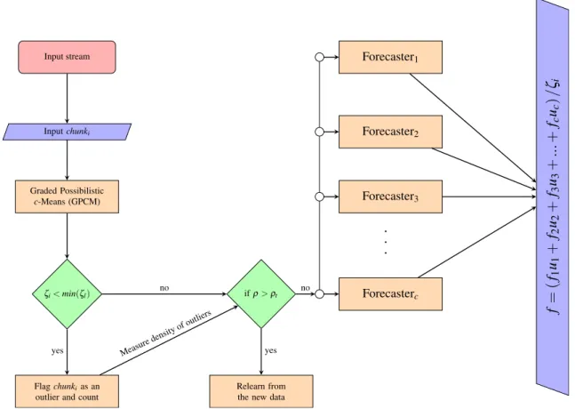
After the training stage, we start the forecasting stage as
shown in Fig.2where chunks come as a stream. For each
upcoming input chunki,fiis computed and compared to a
threshold. In the proposed model, the threshold is selected
as the minimum offlobserved on the training set:
Hmin
l fl: ð19Þ
However, other choices, more or less restrictive, are possible based on the quantity and reliability of the training data.
After the training stage, we start the online forecasting
stage. When a new chunk is presented to RLEM, iff\Hit
is considered an extreme outlier and will be dropped.
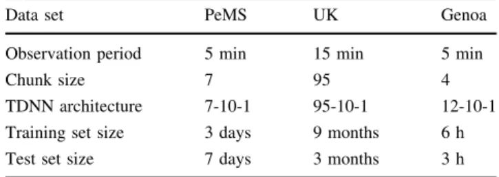
Table 1 RLEM model parameters used for the short-term traffic forecasting for the three data sets
Data set PeMS UK Genoa
Observation period 5 min 15 min 5 min
Chunk size 7 95 4
TDNN architecture 7-10-1 95-10-1 12-10-1 Training set size 3 days 9 months 6 h Test set size 7 days 3 months 3 h
Technically, this is implemented as follows. We
com-pute the binarized membership mass of the input chunk,
defined as:
fB¼ 0 for f\H
1 otherwise
: ð20Þ
The upcoming chunk is considered as an extreme outlier and is dropped (rejected) iffBi ¼0.
The drop rate of the input chunks depends on the value
ofawhich controls the sensitivity of the model to outliers.
A high value ofa-means less sensitivity to outliers and a
lower drop rate.
For detecting concept shift in traffic flows, we use
average densityq as an indicator of the reliability of the
forecasting model.
The final output of the RLEM is computed as a weighted
sum of the individual base learner forecasts [29], as
follows:
f ¼X
c
j¼1
fjuj=f ð21Þ
In Eq. (21), we see that the outputfjof each forecaster is
weighted byuj, which is the membership degree of each
chunk to each cluster, so thatuj will have a high value for
the most suitable forecaster(s) and low to the others.
Note that, despite thepossibilisticnature of the GPCM
method, this weighting is convex (Pjuj=f¼1) because of
the use of f as a partition function, since outliers and
concept drift/shift have been taken into account in the previous layer.
3.6 Retraining
During operation, the system collects a sliding window of a fixed number of past observations from the input stream.
When the outlier densityq is over a certain threshold qt,
the model is considered inadequate and a retraining step is triggered.
In the retraining step, the centroids and forecasters are trained on the current data window, so as to make them up to date.
4 Experiments and Results
The experimental validation of proposed robust layered ensemble model included the test of the clustering
proce-dure based on the Graded Possibilistic c-Means on an
artificial data set with built-in concept drift and shift. Then, we applied RLEM to the short-term forecasting of three traffic flow data sets.
4.1 Data Sets
The data sets employed in our experimental analysis are: • Gaussian data setthat is a synthetic data set with four
evolving two-dimensional Gaussian distributions [12].
Along time, one new data point is added and one removed randomly so that the total number stays constant. However, the underlying data source (cen-troid positions) is slowly changed, leading to concept drift. Concept shift is obtained by removing a whole segment of the sequence at time 4000 where the stream changes abruptly. The data set was generated using the
Matlab program ConceptDriftData.m available at
https://github.com/gditzler/ConceptDriftData.
• PeMS that is a data set by the Caltrans Performance
Measurement System (PeMS) available athttp://pems.
dot.ca.gov. The traffic flow data are collected every 30 s from over 15,000 detectors deployed across Cali-fornia. The collected data are aggregated in 5-min
periods. In [37], a deep learning model was developed
using these data.
• UK road network that contains multiple data sets obtained from different road links in the United
Kingdom (UK) available athttp://www.highways.gov.
uk. This data series provides traffic flow information for
15-min periods since 2009 on most of road links in UK. The data set obtained from the loop sensor id AL2989A (TMU Site 30012533) containing traffic flow between
2009 and 2013 was used in [51] for the validation of
traffic forecasting approach.
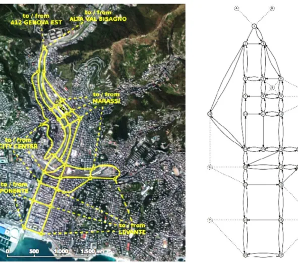
• Genoa Data set containing traffic data of a town obtained via simulation as follows as a part of our
contribution to the PLUG-IN project.1An urban area of
the city of Genoa, a town in the north-west of Italy, was mapped with the aid of Open Street Map data available athttps://www.openstreetmap.org. Traffic parameters were obtained from actual observations and several days of traffic were simulated by using the SUMO open
source traffic simulator [32]. Figure5shows the area of
interest and the graph used to model it which consists of 27 nodes, 74 links, 7 external points and 19 connec-tions. The simulation yielded observations at time intervals of 5 min obtained from a specific link and from a fixed number of adjacent links to forecast the traffic to a short-term timescale.
1 Piattaforma per la mobilita` Urbana con Gestione delle
INfor-mazioni da sorgenti eterogenee (http://www.siitscpa.it/index.php/ progetti/2011-09-24-14-26-55/plug-in).
4.2 Implemented Models
The learning task associated with the Gaussian data set is non-stationary data streaming tracking and outlier detect-ing. We approach this problem using the GPCM clustering model.
Table1 shows the values of parameters of the RLEM
implementations for the short-term traffic forecasting for PeMS, UK and Genoa data sets. Each data corresponds to the average traffic flow measured in the observation period. The size of the data chunk is the time lag estimated as the minimum of the time-delayed mutual information, as
noted in Sect.3.2. The estimated time lags for PeMS, UK
and Genoa data sets correspond, respectively, to 35 min, one day and 20 min.
For the first stage of RLEM that implements a GPCM model for chunk clustering, we set five clusters for all data sets.
The base learners of the second layer of the RLEM are time-delayed neural networks (TDNN) using multilayer perceptrons with three layers. The dimension of the input layer of multilayer perceptrons is identical to the size of the chunk and the hidden layers are set to 10 units for the three cases, while the output is unidimensional and corresponds to estimation of the traffic flow.
4.3 Choice of Parameters
As most adaptive methods, the RLEM model includes three types of parameters: Model parameters, optimization parameters, and evaluation parameters.
Model parameters directly influence the operation of the system in the inference (forecasting) phase. Although the model just described includes several parameters, the only actual, user-selected model parameters are the number of
forecasterscand the topology of the individual forecasters.
When the number of forecasters is increased, it has been observed that the performance of the system increases accordingly, although not proportionally. Additional model parameters influencing the trade-off between stability and reactivity of the system are the adaptation gain for the
moving-average update ofqand the lag periodT. For both
the user can choose an arbitrary value, but reasonable, objective selection criteria have been previously discussed
[Eqs. (16), (2)]. The membership threshold H should
operate on extreme observations. Even if criteria other than
Eq. (19) are employed to set its value, it should not impact
normal operation.
Most parameters described are optimization parameters. These have an indirect influence on the system’s behaviour, being related to the evolution of the system in time. These
Fig. 2 Diagram of the forecasting stage in the RLEM. See text for details on the quantities and on the operational blocks mentioned in the diagram
include initial values for a and b, the size of the initial
windowW0, and the optimization parameters for the
indi-vidual forecasters which depend on the training strategy adopted (in this study, we used the error back-propagation algorithm) but do not have a strong influence on the result due to the use of an ensemble. As for the actual numerical
values of these parameters,ahas an absolute interpretation
and values in [0.85, 1) can be used. However, b strongly
depends on the magnitude, distribution and dimensionality of the data and on the location of clusters, so a general indication cannot be given, although empirical methods like analysing the histogram of pairwise distances between samples can be attempted.
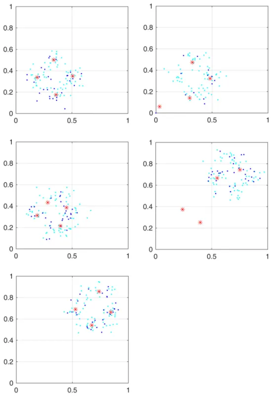
Fig. 3 The five snapshots taken during the clustering process of the Gaussian data set (see Fig.4). In each snapshot, red stars are centroids. Dots are the 100 previous data points, with the 30 most recent in darker colour
Finally, evaluation parameters include the metrics employed to measure performance and the relative size of training set and test set. These do not have a strong influ-ence on the results provided that the metrics are reasonably
related to actual performance on the field, that they are used consistently in comparisons and that the absolute size of training and test set are sufficient. Repeated experiments have shown that this latter point was not an issue with the data sets used in this study.
4.4 Experimental Results and Discussion
4.4.1 Gaussian Data Set
Figure4shows the outlierness indexq(Eq.14) during the
tracking of the Gaussian data set. Five snapshots, taken at
different times, are shown in Fig.3 and labelled with
numbers corresponding to those in Fig.4. Dots represent
the 100 most recent data points of the evolving data set. Stars are the current centroids.
The outlierness index is high when the clustering model does not fit well the data, indicating an inadequacy
situa-tion. Observing the snapshots in Fig.3and referring to the
outlierness indicator in Fig. 4 show that the model can
quickly adapt to the novelty:
Fig. 4 Degree of outlierness during the tracking of the Gaussian data set. The numbers under the curve correspond to the five snapshots in Fig.3
1. After recovering from a moderate drift with respect to initial configuration.
2. After some outliers have appeared (note the fast
recovery of the outlierness indicator in Fig.4).
3. Clusters are changing their relative position but the
data support stays approximately the same. Outlierness slightly increased.
4. Concept shift. The data support changes abruptly from
the south-west to the north-east part of the graph. Outlierness peaks.
5. Recovery from concept shift. Incoming data points are
no longer considered as outliers (Fig.5).
Table 2 Performance
comparison on PeMS data set Methods Index
RMSE Drop rate
SAE 50.0 0
BP-NN 90.2 0 RBF-NN 56.1 0 RLEM 20.8 .0044 Fig. 6 PeMS data set: forecasting results of RLEM (measured values are in blue; forecasted values are in red)
Fig. 7 RLEM model accuracy w.r.tain UK for 3 months
Fig. 8 Results of the two forecasting problems. a Scatter plot between the target and the output (UK data set),bforecast output and the target (Genoa data set). The regression curves are in blue
4.4.2 PeMS
In Fig.6, a forecasting experiment on the traffic flow data
that were used in [37] for comparing the forecasting
capabilities of the stacked autoencoder (SAE), the back-propagation neural network (BP-NN) and the radial basis function neural network (RBF-NN) using three days data for training and the upcoming seven days data for testing. The figure shows the forecasting results obtained by the RLEM using the same training and test sets.
In Table2, we compare forecasting performances of the
models studied in [37] with the RLEM. The performance
indexes used in the table are:
• The mean squared error (MSE) measuring the average
error of the forecasting results:
RMSE¼ ffiffiffiffiffiffiffiffiffiffiffiffiffiffiffiffiffiffiffiffiffiffiffiffiffiffiffiffi 1 N XN i¼1 ðti^tiÞ2 v u u t ; i¼1;. . .;N; ð22Þ
wheretiis the observed traffic value,^tiis its forecasted
value and Nis the size of the test set.
• The drop rate (DR) is defined as follows:
DR¼1 Pi¼N i¼1 f B i N ð23Þ
With a drop of 9 outliers corresponding to a
DR¼.0044, the RLEM shows the best root mean squared
error.
4.4.3 UK and Genoa Data Sets
Figure7 shows the effect of a on the accuracy (mean
square error) of the RLEM model for the UK road network
data set. The selected range ofavalues are:93 a 1. An
appropriate value of a allows us to control the degree of
outlierness, drop unwanted outliers and improve the
accuracy rate. The values of the RMS are very small, but this magnitude depends on the range of the data. What carries useful information is actually the change in these values, i.e. the relative differences between values.
Figure8 shows the scatter plots of the traffic flow
forecasting using the UK road network data set (a), and the one for Genoa data set (b), both with zero drop rate. The correlation coefficients are, respectively, .98 and .99.
Fig-ure9shows data from the UK data set as a continuous line,
with forecast output superimposed as round dots, with a
similar representation as in Fig.6.
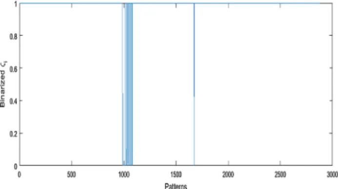
Figure10 shows the binarized mass of membership fBi
for the chunks of the test set. Where the value offBi drops
the forecasting performance decreases, because the data are
not well explained by the model. This makes fBi a good
indicator of model reliability and forecasting performance even during the inference phase, i.e. when targets are not available.
5 Conclusions
In this paper, we have proposed the RLEM model for short-term traffic flow forecasting. The model combines the graded possibilistic c-means clustering and ensembles of time-delayed neural networks and uses an outlierness density index to measure the reliability of the forecaster model.
We evaluated the performance of clustering model on synthetic data set, for which the ground truth is available, and then we evaluated the performance of RLEM model on three data sets. For the PeMS data set, we compared our results with SAE, BP NN and RBF NN models, and the results show that the proposed method gives an accurate forecasting of the traffic flow rates with outlier detection and shows a good adaptation to non-stationary traffic regimes. For the UK data sets, we show that the proper
selection ofa improves the forecasting accuracy.
Fig. 9 Forecasted output and the target on the UK data set with 0 drop rate
Fig. 10 Binarized sum of membership of each chunk to all clusters during a run on the UK data set
Given its characteristics of outlier detection, accuracy and robustness, RLEM can be fruitfully integrated into real-time traffic flow management systems.
Open Access This article is distributed under the terms of the Creative Commons Attribution 4.0 International License (http://crea tivecommons.org/licenses/by/4.0/), which permits unrestricted use, distribution, and reproduction in any medium, provided you give appropriate credit to the original author(s) and the source, provide a link to the Creative Commons license, and indicate if changes were made.
References
1. Abdullatif A, Rovetta S, Masulli F (2016) Layered ensemble model for short-term traffic flow forecasting with outlier detec-tion. In: 2016 IEEE 2nd international forum on research and technologies for society and industry leveraging a better tomor-row (RTSI), pp 1–6. doi:10.1109/RTSI.2016.7740573
2. Aggarwal CC (2006) Data streams: models and algorithms (ad-vances in database systems). Springer, Secaucus
3. Aggarwal CC (2007) Data streams: models and algorithms, vol 31. Springer, Berlin
4. Aggarwal CC, Han J, Wang J, Yu PS (2003) A framework for clustering evolving data streams. In: Proceedings of the 29th international conference on very large data bases, vol 29, VLDB ’03, pp 81–92. VLDB Endowment
5. Aggarwal CC, Yu PS (2008) A framework for clustering uncer-tain data streams. In: Proceedings of the 2008 IEEE 24th inter-national conference on data engineering, ICDE ’08. IEEE Computer Society, Washington, pp 150–159
6. Amini A, Wah T, Saboohi H (2014) On density-based data streams clustering algorithms: a survey. J Comput Sci Technol 29(1):116–141. doi:10.1007/s11390-014-1416-y
7. Barbara´ D, Domeniconi C, Duric Z, Filippone M, Mansfield R, Lawson E (2008) Detecting suspicious behavior in surveillance images. In: Data mining workshops, 2008. ICDMW’08. IEEE international conference on. IEEE, pp 891–900
8. Bezdek JC (1981) Pattern recognition with fuzzy objective function algorithms. Kluwer, Norwell
9. Can F (1993) Incremental clustering for dynamic information processing. ACM Trans Inf Syst 11(2):143–164. doi:10.1145/ 130226.134466
10. Casdagli M, Eubank S, Farmer J, Gibson J (1991) State space reconstruction in the presence of noise. Phys D Nonlinear Phe-nom 51(1):52–98. doi:10.1016/0167-2789(91)90222-U
11. Chandola V, Banerjee A, Kumar V (2009) Anomaly detection: a survey. ACM Comput Surv (CSUR) 41(3):15
12. Ditzler G, Polikar R (2013) Incremental learning of concept drift from streaming imbalanced data. IEEE Trans Knowl Data Eng 25:2283–2301
13. Ester M, peter Kriegel H, Sander J, Xu X (1996) A density-based algorithm for discovering clusters in large spatial databases with noise. In: KDD. AAAI Press, pp 226–231
14. Faraway J, Chatfield C (1998) Time series forecasting with neural networks: a comparative study using the airline data. Appl Stat 47:231–250
15. Filippone M, Masulli F, Rovetta S (2010) Applying the possi-bilistic c-means algorithm in kernel-induced spaces. IEEE Trans Fuzzy Syst 18:572–584
16. Fowe AJ, Chan Y (2013) A microstate spatial-inference model for network-traffic estimation. Transp Res Part C Emerg Technol 36:245–260
17. Fraser AM, Swinney HL (1986) Independent coordinates for strange attractors from mutual information. Phys Rev A 33:1134–1140. doi:10.1103/PhysRevA.33.1134
18. Gao J, Leng Z, Qin Y, Ma Z, Liu X (2013) Short-term traffic flow forecasting model based on wavelet neural network. In: 2013 25th Chinese control and decision conference (CCDC), pp 5081–5084. doi:10.1109/CCDC.2013.6561856
19. Gao Y, Sun S (2010) Multi-link traffic flow forecasting using neural networks. In: 2010 Sixth international conference on nat-ural computation, vol 1, pp 398–401. doi:10.1109/ICNC.2010. 5582914
20. Gao Y, Sun S, Shi D (2011) Network-Scale Traffic Modeling and Forecasting with Graphical Lasso. In: Liu D, Zhang H, Poly-carpou M, Alippi C, He H (eds) Advances in Neural Networks– ISNN 2011: 8th International Symposium on Neural Networks, Guilin, China, 2011, vol 6676. Springer, Berlin, Heidelberg. doi:10.1007/978-3-642-21090-7_18
21. Ghosh B, Basu B, O’Mahony M (2009) Multivariate short-term traffic flow forecasting using time-series analysis. IEEE Trans Intell Transp Syst 10(2):246–254
22. Giglio D (2015) A medium-scale network model for short-term traffic prediction at neighbourhood level. In: 2015 IEEE 18th international conference on intelligent transportation systems, pp 1388–1395 (2015). doi:10.1109/ITSC.2015.228
23. Hamed M, AI-Masaeid H, Bani Said Z (1995) Short-term pre-diction of traffic volume in urban arterials. J Transp Eng 121:249–254
24. Han J, Kamber M, Pei J (2011) Data mining: concepts and techniques, 3rd edn. Morgan Kaufmann, San Francisco 25. Havens T, Bezdek J, Leckie C, Hall L, Palaniswami M (2012)
Fuzzy c-means algorithms for very large data. IEEE Trans Fuzzy Syst 20(6):1130–1146. doi:10.1109/TFUZZ.2012.2201485 26. Hore P, Hall L, Goldgof D (2007) Creating streaming iterative
soft clustering algorithms. In: Fuzzy information processing society, 2007. NAFIPS ’07. Annual Meeting of the North American, pp 484–488
27. Hore P, Hall L, Goldgof D (2007) Single pass fuzzy c means. In: Fuzzy systems conference, 2007. FUZZ-IEEE 2007. IEEE international, pp 1–7. doi:10.1109/FUZZY.2007.4295372 28. Hore P, Hall L, Goldgof D, Cheng W (2008) Online fuzzy c
means. In: Fuzzy information processing society, 2008. NAFIPS 2008. Annual meeting of the North American, pp 1–5. doi:10. 1109/NAFIPS.2008.4531233
29. Jacobs RA, Jordan MI, Nowlan SJ, Hinton GE (1991) Adaptive mixtures of local experts. Neural Comput 3(1):79–87. doi:10. 1162/neco.1991.3.1.79
30. Kantz H, Schreiber T (2003) Nonlinear time series analysis, 2nd edn. Cambridge University Press, Cambridge
31. Kaufman L, Rousseeuw PJ (2005) Finding groups in data: an introduction to cluster analysis (Wiley Series in Probability and Statistics), 1st edn. Wiley-Interscience, New York
32. Krajzewicz D, Erdmann J, Behrisch M, Bieker L (2012) Recent development and applications of sumo—simulation of urban mobility. Int J Adv Syst Meas 5:128–138
33. Krishnapuram R, Joshi A, Yi L (1999) A fuzzy relative of the k-medoids algorithm with application to web document and snippet clustering. In: Fuzzy systems conference proceedings, 1999. FUZZ-IEEE ’99. 1999 IEEE international, vol 3, pp 1281–1286. doi:10.1109/FUZZY.1999.790086
34. Krishnapuram R, Keller JM (1993) A possibilistic approach to clustering. IEEE Trans Fuzzy Syst 1(2):98–110
35. Krishnapuram R, Keller JM (1996) The possibilistic C-means algorithm: insights and recommendations. IEEE Trans Fuzzy Syst 4(3):385–393
36. Labroche N (2010) New incremental fuzzy c medoids clustering algorithms. In: Fuzzy information processing society (NAFIPS),
2010 annual meeting of the North American, pp 1–6. doi:10. 1109/NAFIPS.2010.5548263
37. Lv Y, Duan Y, Kang W, Li Z, Wang FY (2015) Traffic flow prediction with big data: a deep learning approach. IEEE Trans Intell Transp Syst 16(2):865–873. doi:10.1109/TITS.2014. 2345663
38. Masulli F, Rovetta S (2006) Soft transition from probabilistic to possibilistic fuzzy clustering. IEEE Trans Fuzzy Syst 14(4):516–527. doi:10.1109/TFUZZ.2006.876740
39. Mei JP, Chen L (2010) Fuzzy clustering with weighted medoids for relational data. Pattern Recogn 43(5):1964–1974. doi:10. 1016/j.patcog.2009.12.007
40. Ng RT, Han J (2002) Clarans: a method for clustering objects for spatial data mining. IEEE Trans Knowl Data Eng 14(5):1003–1016
41. Robbins H, Monro S (1951) A stochastic approximation method. Ann Math Stat 22(3):400–407. doi:10.1214/aoms/1177729586 42. Rose K, Gurewitz E, Fox G (1990) A deterministic annealing
approach to clustering. Pattern Recogn Lett 11:589–594 43. Schlimmer J, Granger RH (1986) Incremental learning from
noisy data. Mach Learn 1(3):317–354. doi:10.1007/BF00116895 44. Stathopoulos A, Dimitriou L (2008) Fuzzy modeling approach for combined forecasting of urban traffic flow. Comput-Aided Civ Infrastruct Eng 23:521
45. Sun S (2009) Traffic flow forecasting based on multitask ensemble learning. In: Proceedings of the first ACM/SIGEVO summit on genetic and evolutionary computation, GEC ’09. ACM, New York, pp 961–964. doi:10.1145/1543834.1543984 46. Treiber M, Kesting A (2012) Validation of traffic flow models
with respect to the spatiotemporal evolution of congested traffic patterns. Transp Res Part C Emerg Technol 21(1):31–41 47. Tselentis D, Vlahogianni E, Karlaftis M (2015) Improving
short-term traffic forecasts: to combine models or not to combine? IET Intell Transp Syst 9(2):193–201. doi:10.1049/iet-its.2013.0191 48. Vlahogianni EI, Karlaftis MG, Golias JC (2014) Short-term
traffic forecasting: where we are and where we’re going. Transp Res Part C Emerg Technol 43:3
49. Vythoulkas P (1992) Alternative approaches to short-term traffic forecasting for use in driver information systems. In: Interna-tional symposium on the theory of traffic flow and transportation (12th: 1993: Berkeley). Transportation and traffic theory 50. Wang Y, Chen L, Mei JP (2014) Incremental fuzzy clustering
with multiple medoids for large data. IEEE Trans Fuzzy Syst 22(6):1557–1568. doi:10.1109/TFUZZ.2014.2298244
51. Wibisono A, Jatmiko W, Wisesa HA, Hardjono B, Mursanto P (2016) Traffic big data prediction and visualization using fast incremental model trees-drift detection (FIMT-DD). Knowl-Based Syst 93:33–46
52. Yin H, Wong SC, Xu J, Wong CK (2002) Urban traffic flow prediction using a fuzzy-neural approach. Transp Res Part C Emerg Technol 10:85–98
53. Yoon B, Chang H (2014) Potentialities of data-driven nonpara-metric regression in urban signalized traffic flow forecasting. J Transp Eng 140(04014):027
54. Yoon KA, Kwon OS, Bae DH (2007) An approach to outlier detection of software measurement data using the k-means clustering method. In: Empirical software engineering and mea-surement, 2007. ESEM 2007. First international symposium on. IEEE, pp 443–445
55. Zhang T, Ramakrishnan R, Livny M (1996) Birch: An efficient data clustering method for very large databases. In: Proceedings of the 1996 ACM SIGMOD international conference on man-agement of data, SIGMOD ’96. ACM, New York, pp 103–114 56. Zhang Y (2011) Hourly traffic forecasts using interacting
multi-ple model (IMM) predictor. IEEE Signal Process Lett 18:607–610
57. Zhao G, Li Z, Liu F, Tang Y (2013) A concept drifting based clustering framework for data streams. In: Emerging intelligent data and web technologies (EIDWT), 2013 fourth international conference on, pp 122–129. doi:10.1109/EIDWT.2013.26 58. Zliobaite I, Bifet A, Pfahringer B, Holmes G (2014) Active
learning with drifting streaming data. IEEE Trans Neural Netw Learn Syst 25(1):27–39. doi:10.1109/TNNLS.2012.2236570