HAL Id: hal-01768646
https://hal.archives-ouvertes.fr/hal-01768646
Submitted on 17 Apr 2018
HAL
is a multi-disciplinary open access
archive for the deposit and dissemination of
sci-entific research documents, whether they are
pub-lished or not. The documents may come from
teaching and research institutions in France or
abroad, or from public or private research centers.
L’archive ouverte pluridisciplinaire
HAL
, est
destinée au dépôt et à la diffusion de documents
scientifiques de niveau recherche, publiés ou non,
émanant des établissements d’enseignement et de
recherche français ou étrangers, des laboratoires
publics ou privés.
A comparison of different routing schemes for the robust
network loading problem: polyhedral results and
computation
Sara Mattia, Michael Poss
To cite this version:
Sara Mattia, Michael Poss. A comparison of different routing schemes for the robust network
load-ing problem: polyhedral results and computation. Computational Optimization and Applications,
Springer Verlag, 2018, 69 (3), pp.753 - 800. �10.1007/s10589-017-9956-z�. �hal-01768646�
A comparison of different routing schemes for the robust
network loading problem: polyhedral results and computation
Sara Mattia
∗Michael Poss
†Abstract
We consider the capacity formulation of the Robust Network Loading Problem. The aim of the paper is to study what happens from the theoretical and from the computational point of view when the routing policy (or scheme) changes. The theoretical results consider static, volume, affine and dynamic routing, along with splittable and unsplittable flows. Our polyhedral study provides evidence that some well-known valid inequalities (the robust cutset inequalities) are facets for all the considered routing/flows policies under the same assumptions. We also intro-duce a new class of valid inequalities, the robust 3-partition inequalities, showing that, instead, they are facets in some settings, but not in others. A branch-and-cut algorithm is also proposed and tested. The computational experiments refer to the problem with splittable flows and the budgeted uncertainty set. We report results on several instances coming from real-life networks, also including historical traffic data, as well as on randomly generated instances. Our results show that the problem with static and volume routing can be solved quite efficiently in practice and that, in many cases, volume routing is cheaper than static routing, thus possibly repre-senting the best compromise between cost and computing time. Moreover, unlikely from what one may expect, the problem with dynamic routing is easier to solve than the one with affine routing, which is hardly tractable, even using decomposition methods.
Keywords: robust network loading, budgeted uncertainty, Benders decomposition, static rout-ing, volume routrout-ing, affine routrout-ing, dynamic routing.
1
Introduction
Given an undirected graph and a set of point-to-point commodities with known demands (traffic matrix), the objective of the network design problem is to find the cheapest capacity installation on the edges of the graph such that the resulting network supports the routing of the commodities. The problem has numerous applications in telecommunications, transportation, and energy management, among many others. Accordingly, a large number of variations can be defined, which restrict for instance, the type of flows admissible on the edges or the type of capacities that can be installed on the edges. A large variety of technical constraints can also be considered. They include ensuring a given level of survivability in case of link failures or limiting the length of the paths used. Different flows policies may be used: the demands may be restricted to be routed on single paths (unsplit-table flows) or the flows may be unrestricted (split(unsplit-table flows) [9]. Herein, we focus on the so-called Network Loading Problem, where capacities can be installed by integer multiples. An important aspect of network design problems is related to the knowledge of the demands. In a large number of applications, these demands are not available at the time we decide on the capacity installation. Here we refer to the Network Loading Problem under uncertain demands as the Robust Network Loading Problem. A way to deal with demand uncertainty is to rely on demand forecasts, based, for instance, on population statistics [18] or on traffic measurements [48]. If these statistical studies are accurate enough, one can come up with a stochastic model that considers demands as known random ∗S. Mattia. Istituto di Analisi dei Sistemi ed Informatica. Consiglio Nazionale delle Ricerche. Via dei Taurini 19,
00185 Roma (Italy). Email: [email protected].
†M. Poss. UMR CNRS 5506 LIRMM. Universit´e de Montpellier. Rue Ada 161, 34095 Montpellier cedex 5, (France).
variables, typically leading to two-stage stochastic programs. See [5] and the references therein for additional details. Unfortunately, it is very difficult in practice to come up with an accurate de-scription of these random variables. An alternative approach is to define sets of admissible values of random variables compatible with the available data, falling into the framework of distributionally robust optimization [46]. In this work, we assume that the uncertain demands are described through an uncertainty set [11], falling into the framework of robust optimization [13]. Hence, the problem turns to designing a network able to route each traffic matrix in the uncertainty set. Although conservative, this approach has been used extensively in recent years to model demand uncertainty in telecommunications and transportation networks [4, 8, 26, 33, 34, 37, 38, 44]. A popular choice to model the forecast demands is to use the budgeted uncertainty set [15]. The latter supposes that the demands fluctuate between their nominal values and given peak values and that at most Γ of them reach their peak values simultaneously. The model is motivated by probabilistic guarantees [15] and has been used in numerous papers on robust network design problems [8, 34, 44].
The introduction of uncertainty in demands raises the question of how to adapt the flows to dif-ferent realizations of the demand. This concept is often referred to as routing in the literature on network optimization. Different routing policies (or schemes) have been studied in the past, each with its own flexibility and computational issues [4, 33, 44]. At one extreme, we findstatic routing, which imposes that the fractional splitting of the commodities among a fixed set of paths stays constant for all realizations of the demands. In the other extreme,dynamic routing allows the flows to be changed completely any time that the demands change. Both approaches have advantages and drawbacks. Dynamic routing is more flexible, but the corresponding problem is difficult to solve. In addition, dynamic routing can be difficult to implement in practice because the routing depends on the current status of all the demands in the network, thus, hardening decentralization. On the other hand, static problems are usually computationally more tractable and easier to implement in decentralized environments, but the corresponding solutions may be too conservative. Therefore, in the last years, several intermediate routing schemes have been proposed. They include affine and volume routing. The aim was to obtain more flexibility than static routing, solving a problem that is theoretically easier than the dynamic one. Affine routing [41] restricts the flows to be affine functions of the demands, as it applies to network optimization what has long been known as affine decision rules in adjustable robust optimization [14]. Affine routing has been used in several papers on robust network design, see for instance [8, 28, 40, 44], including a variation of the problem where it is the capacity, rather than the demand, which is uncertain [42]. Volume routing [12] is a special case of affine routing, where the set of paths used for each commodity can be adjusted according to the current value of the demand for that commodity. In addition to its numerical tractability, volume routing is easier to implement in a decentralized environment than affine and dynamic routing, since the routing for a commodity only depends on the demand for that commodity. Other intermediate routings have also been proposed in the literature, such as those based on dynamic partitions of the uncertainty set [10, 45]. However, they lead to optimization problems that are even harder to solve than the problem with dynamic routing [43]. For this reason, we do not consider them in what follows. The computational tractability of the Robust Network Loading Problem has been studied under static, affine and dynamic routing. The problem is N P-hard independently of the routing scheme, as it includes the problem without uncertainty, and then the Steiner tree problem, as a special case. However, even for the splittable case, when the integrality restrictions on the capacity variables are relaxed, the complexity of the problem does depend on the routing. For affine, volume and static routing there exists a compact formulation, that is, a formulation with a polynomial number of variables and constraints, and, hence, the problem can be solved in polynomial time [3, 12, 44]. In contrast, the problem with dynamic routing was proved to beN P-hard, both in general and for the budgeted uncertainty set [20, 25, 36]. Therefore, no compact formulation exists, unless P =N P. As a consequence, for static/affine/volume routing separation is polynomial, whereas for dynamic routing it isN P-hard [33]. This affects the computational performance of the problem with integer capacities. For splittable flows and static routing, in [4] the authors propose a polyhedral investiga-tion and numerical results for the problem assuming that the demand uncertainty polytope is the Hose model [22, 23]. Similar numerical studies have been carried out in [26] for the problem with
budgeted uncertainty. In [27] a Benders decomposition approach for the splittable Robust Network Loading Problem with static routing and budgeted uncertainty is derived and studied. In [33] the author studies the problem with dynamic routing and splittable flows under the Hose model, propos-ing a branch-and-cut procedure related to bilevel optimization. A special case of that problem is studied in [19], where the authors focus on single-commodity problems, which allows them to provide more efficient inequalities and separation routines. Finally, in [37] the problem with splittable flows, affine routing and polyhedral or ellipsoidal uncertainty sets is studied. The authors further consider a version of the problem with restrictions on the set of feasible paths and propose column generation algorithms.
In this paper we study the capacity formulation of the Robust Network Loading Problem, that is, a formulation including only design variables. The scope of the paper is to investigate what happens both theoretically and computationally when the routing policy changes. To the best of our knowl-edge, this is the first time that such a comprehensive investigation is carried out. From the theoretical point of view, a first contribution of the paper is to derive a capacity formulation for the problem with volume and affine routing using a Benders decomposition approach. For dynamic routing, the exponential number of variables and constraints in the formulation prevents us from using the flow formulation as a starting point for deriving a capacity formulation, and hence, from applying the classical Benders reformulation. Instead, we must draw from the more advanced tools proposed in the recent years for adjustable robust optimization, see [7, 33, 47]. We refer to the formulations in-cluding only design variables as Benders formulations in the rest of the paper, despite the differences in the techniques used to obtain them. We provide polyhedral results characterizing the convex-hull of integer feasible solutions of the problem for all the considered routing schemes under splittable and unsplittable flows, for a general uncertainty set. We establish relations among the polyhedra corresponding to the considered routing schemes, giving conditions for an inequality that is valid or facet under a given routing/flows policy pair to be valid or facet for another routing/flows pair. Following the comments in [33], we formally prove that the well-known robust cutset inequalities [26, 33, 34] are facets under the same assumptions in all the considered settings. Actually, this is, so far, the only class of inequalities having such a property, but for the non-negativity constraints. Indeed, we present a new class of valid inequalities for the Robust Network Loading Problem, the robust 3-partition inequalities, and show that they are facet-defining for the problem with dynamic routing and splittable flows, whereas they are not facets, under the same assumptions, for the other routing schemes or for unsplittable flows. They provide the first example of such a behavior. From a computational perspective, we investigate what is the effect of the different routing schemes on costs and computing times, when the splittable problem is solved using the budgeted uncertainty set, the Benders formulations and the cuts investigated in the theoretical part. We provide exact and heuristic separation routines for the robust cutset inequalities, a heuristic approach for finding a violated robust 3-partition inequality, an exact approach for the Benders cuts and a primal heuristic. We compare the Benders formulations using many different cutting plane approaches. We also in-vestigate the compact flow formulation for volume, affine and static routing. Although compact, the corresponding problem may be time consuming for some of the considered routing schemes. How-ever, we show that its performance can be significantly improved by separating the above mentioned inequalities in the branch-and-cut tree. We report computational experiments on real-life instances, including instances based on historical traffic data [39], as well as on randomly generated ones. We prove that the problem with static and volume routing can be solved quite efficiently in practice on the considered instances. Moreover, unlikely from what one may expect, the problem with dynamic routing is easier to solve than the one with affine routing. It turns out that all the considered routing schemes (but possibly affine routing) are able to solve real-life problems. We also show that volume routing yields cost reductions over static routing in half of the instances, while not requiring more computational time. This is important because many papers use static routing, whereas volume routing is not so popular.
The paper is structured as follows. Sections 2 and Section 3 present, respectively, the so-called flow and Benders formulations of the Robust Network Loading Problem for each of the aforementioned routing schemes. In Section 4 we give polyhedral results. In Section 5 we present implementation
details and the test-bed. In Sections 6 we discuss computational experiments. The paper is concluded in Section 7. When presenting models and computational results (Sections 2, 3, 5, 6), we restrict to splittable flows and to the budgeted uncertainty set, whereas the theoretical results (Section 4) are more general and they also hold for unsplittable flows and are independent of the uncertainty set.
2
Flow formulations
LetG(V, E) be an undirected graph without loops and parallel edges, letK be the set of point-to-point commodities to be routed on the network and assume that all the demands belonging to a given uncertainty set U ⊂R|+K| must be served. Each commodity k∈K is defined by its endnodes
sk and tk and its demand value dk for any d∈ U. In presenting the models, we suppose that the
flows are splittable and that the uncertainty set has a special structure, often used in the literature [15]: each demand value dk varies between its nominal value ¯dk and its peak value ¯dk+ ˆdk and the
number of deviations from the nominal value is bounded by integer Γ. It corresponds to the extended formulation below and we denote it byUb.
Ub≡ ( d∈R|+K|| ∃δ∈[0,1]|K|:dk = ¯dk+δkdˆk, k∈K, X k∈K δk≤Γ ) (1)
In what follows we use U when the formulation or the result refers to a general uncertainty set, whereas we useUb when we specifically refer to the budgeted uncertainty set. We do not make any
special assumption on U, but that it is bounded (otherwise the resulting problem is unbounded) and non-empty (otherwise the resulting problem is trivial). By non-empty we also mean thatU is different from the singleton{0}, as the resulting problem admits the trivial solutionx=0, as well. We associate to E the set of directed arcsA: for each e ={i, j} ∈E, we create two directed arcs (i, j) and (j, i). The unitary cost of installing capacity on edgee ∈E is given by ce. The Robust
Network Loading Problem studied herein aims at installing the cheapest capacities xon the edges of the graph, such that all realizations of the demand vectorsd∈ U can be routed on the resulting network.
2.1
Dynamic routing
The problem with dynamic routing can be formulated mathematically as follows. The integer variable
xerepresents the capacity allocation on edgee∈Eand the real variablefijk(d) describes the amount
of flow for commodityk routed on arc (i, j)∈A, when considering demandd∈ U. We also define the star of nodei∈N asN(i) ={j∈N :∃e={i, j} ∈E}.
f DRN L min X e∈E cexe s.t. X j∈N(i) (fjik(d)−fijk(d)) = dk ifi=tk 0 otherwise i∈V \ {sk}, k∈K,d∈ U (2a) X k∈K (fijk(d) +fjik(d))≤xe e={i, j} ∈E,d∈ U (2b) f,x≥0 (2c) x∈Z|E| (2d)
Constraints (2a) represent flow conservation constraints at every node of the network (constraints for sk are not included because they are redundant) and constraints (2b) impose that the amount
of flow on each edge does not exceed the available capacity on that edge. In the following, we call routingthe flow functionf. We use the termdynamic routingwhen no particular assumption is made on admissible functions, as in f DRN L. Problem f DRN L is a mixed integer linear programming problem with an infinite number of variables and constraints. However, we see easily that the problem can be discretized by considering the extreme points of the demand polyhedron, denoted by vert(U),
yielding a finite mixed-integer linear formulation. However, when some uncertainty sets are used, the resulting formulation is extremely large, since the number of extreme points of U may grow exponentially. This is the case forUb, where
|vert(Ub)|= Γ X l=0 Γ l .
One way to cope with such a large formulation is to use a decomposition approach to generate only a subset of the extreme points on the fly in the course of branch-and-cut algorithms. We explain in the next section how Benders decomposition can be used to do that. Alternatively, we could restrict the routing to simple functions of d.
2.2
Affine routing
Rather than lettingf be an arbitrary function ofd, we can enforce that the following restrictions be satisfied.
fijk(d) =fij0k+
X
h∈K
ykhijdh k∈K,(i, j)∈A. (3)
Constraints (3) yields what is known as affine decision rule oraffine routing in the literature [40, 41, 44]. The constraints limitf to be an affine function of d. Here we explain how to obtain a compact reformulation for the affine problem from f DRN L using constraints (3) and linear programming duality, for Ub. The reader is referred to [44] for further details. Plugging (3) intof DRN Lyields
min X e∈E cexe s.t. X j∈N(i) fij0k+X h∈K yijkhdh−(fij0k+X h∈K ykhij dh) ! = dk ifi=tk 0 otherwise i∈V \ {sk}, k∈K,d∈ U (4a) X k∈K fij0k+ X h∈K ykhij dh+fji0k+ X h∈K ykhjidh ! ≤xe e={i, j} ∈E, d∈ U (4b) fij0k+X h∈K ykhij dh≥0 (i, j)∈A, k∈K (4c) x≥0,x∈Z|E| (4d)
Consider first equations (4a) and group the terms according to their dependency on d. Then, we consider ¯d+eh whereeh
h= 1 ande h
k = 0 for eachk6=h. Subtracting (4a) written for ¯dfrom (4a)
written for ¯d+eh yields the reformulation (6a)–(6c). Consider now constraints (4b) and use the
definition dk = ¯dk+δkdˆk. They can be rewritten as
X k∈K (fij0k+fji0k) +X h∈K ¯ dhX k∈K (yijkh+ykhji) + max δ∈[0,1]|K|:P hδh≤Γ X h∈K δhdˆhX k∈K (ykhij +yjikh)≤xe. (5)
Replacing the inner maximization problem of (5) by its dual yields (6d) and (6e), where zeand pke
are the dual variables corresponding to constraintsP
hδ
h≤Γ andδk ≤1, respectively. Proceeding
similarly with (4c) yields (6f) and (6g). Then, the flow formulation of the affine problem is the following. f ARN L min X e∈E cexe s.t. X j∈N(i) (yijk −y k ji) = 1 ifi=tk 0 otherwise i∈V \ {sk}, k∈K (6a)
X j∈N(i) (yjikh−ykhij ) = 0 i∈V \ {sk}, k6=h∈K (6b) X j∈N(i) (fji0k−fij0k) = 0 i∈V \ {s k}, k∈K (6c) Γze+ X k∈K pke+fij0k+fji0k+X h∈K (ykhij +yjikh) ¯dh ! ≤xe e={i, j} ∈E (6d) ze+pke ≥ X k∈K (yijkh+yjikh) ˆdh e={i, j} ∈E, h∈K (6e) Γsij−fij0k+ X h∈K qijkh−y kh ij d¯ h ≤0 (i, j)∈A, k∈K (6f) sij+qijkh≥y kh ij dˆ h (i, j)∈A, k∈K, h∈K (6g) z,s,p,q,x≥0 (6h) x∈Z|E| (6i)
Variables z,s,p,q come from dualizing the robust constraints, whereas f0 and y come from the
restrictions imposed to the routing by (3). Although compact, formulation f ARN Lis quadratic in
|K|, which makes the problem significantly harder to solve than its deterministic counterpart. As we will show in our numerical experiments, the dimension of the reformulation is such that it even its linear programming relaxation can hardly be solved in reasonable amounts of time. To avoid this quadratic dependency on |K|, we can consider special cases of affine routing that contain less degrees of freedom than (3). Below we present two such cases and we show how the corresponding formulations can be derived fromf ARN L.
2.3
Volume routing
We enforcef to satisfy
fijk(d) =fij0k+yijkkdk, k∈K,(i, j)∈A (7) obtaining a subclass of affine routing known asvolume routing. Roughly speaking, (7) means that the flows are defined by a set of paths froms(k) tot(k) (associated withy), modified by the circulation described by f0. Volume routing has been originally introduced in [12]. Plugging constraints (7) into f DRN L and applying the techniques mentioned above, yields the following reformulation for the problem: f V RN L min X e∈E cexe s.t. X j∈N(i) (ykji−ykij) = 1 ifi=tk 0 otherwise i∈V \ {sk}, k∈K (8a) X j∈N(i) (fji0k−fij0k) = 0 i∈V \ {sk}, k ∈K (8b) Γze+ X k∈K pke+fij0k+fji0k+ (yijkk+yjikk) ¯dk ≤xe e={i, j} ∈E (8c) ze+pke ≥(y kk ij +y kk ji) ˆd k e={i, j} ∈E, k∈K (8d) fij0k+yijkkd¯k ≥0 (i, j)∈A, k∈K (8e) fij0k+yijkk( ¯dk+ ˆdk)≥0 (i, j)∈A, k∈K (8f) z,p,x≥0 (8g)
x∈Z|E| (8h)
Formulation (8) can be derived from formulation (6) by removing flow conservation constraints (6c), replacing robust non-negativity constraints (6f) and (6g) by (8e) – (8f) and removing the terms corresponding toykhforh6=kin robust capacity constraints (6d) – (6e). Notice that other authors
have proposed different restrictions of affine routing to reduce the size of the reformulation [8].
2.4
Static routing
We enforcef to satisfy
fijk(d) =ykkijdk, k∈K,(i, j)∈A, (9) obtaining a subclass of volume routing, known as static routing. Static routing is a well-known framework for the Robust Network Loading Problem and it has been studied long before affine routing was introduced [22, 23]. When constraints (9) are satisfied, variables y are often called routing template, because they represent the fractional splittings of demands along the paths fromsk
totk for eachk∈K. Plugging constraints (9) intof DRN Land applying the techniques mentioned
above, yields the following reformulation for the problem:
f SRN L min X e∈E cexe s.t. X j∈N(i) (ykji−ykij) = 1 ifi=tk 0 otherwise i∈V \ {s k}, k∈K (10a) Γze+ X k∈K pke+ (yijkk+yjikk) ¯dk ≤xe e={i, j} ∈E (10b) ze+pke ≥(y kk ij +y kk ji) ˆd k e={i, j} ∈E, k∈K (10c) z,p,y,x≥0 (10d) x∈Z|E| (10e)
Formulation (10) can be derived from formulation (6) by removing flow conservation constraints (6b) – (6c), replacing robust non-negativity constraints (6f) – (6g) byy≥0and removing the terms corresponding tof0 andykhforh6=kin robust capacity constraints (6d) – (6e).
3
Benders formulations
Benders decomposition is a technique that projects out (part of) the continuous variables of a mixed integer linear programming problem, replacing them by a possibly exponential number of cutting planes that define the feasibility polyhedron for the variables that are not projected out. The cutting planes are usually generated on the fly in the course of branch-and-cut algorithms. It has been applied to many problems, ranging from black-out prevention [17] to shift-scheduling [35]. A standard choice in solving networks design problems consists of projecting out the flow variables working on a master problem which includes only the design variables (see [1, 6, 27, 31, 32, 33] and references therein). This corresponds to the practical decomposition of the decision process: in fact, the design variables correspond to long term decisions, whereas the flow variables correspond to decisions taken at the operational level (short term decisions). We explain in this section how to apply Benders decomposition to f DRN Land f ARN L. This is the first formal presentation of a Benders formulation for the problem with affine (and volume) routing. Benders reformulations for dynamic and static routing can be found in [27, 33]. We point out that the purposes of using Benders decomposition are different forf DRN Landf ARN L. Forf ARN L(and its simplifications
f SRN Landf V RN L), Benders decomposition avoids solving a large linear program at each node of the branch-and-bound tree. For f DRN L, the mixed integer linear programming problem contains exponentially many variables and constraints (and we know from itsN P-hardness that no compact formulation exists). Hence, the use of Benders decomposition avoids to consider explicitly all vectors in vert(U), as needed extreme points are generated on the fly by solving a separation problem.
3.1
Affine routing and simplifications
We project the flow variables out of formulation (6). Let Baf f be the projection of the set defined
by constraints (6a)–(6h), formally:
Baf f ≡ {x∈
R|E|:∃f0,y,z,s,p,q that satisfy (6a)−(6h)}.
Different approaches can be used to test whether a given vectorxbelongs toBaf f. In the following,
we use a reformulation based on strong linear programming duality. In this end, given ¯x∈R|+E|, we
introduce the feasibility problem associated with ¯x
F easAf f(¯x) minα s.t. X j∈N(i) (ykij−yjik) = 1 ifi=tk 0 otherwise i∈V \ {sk}, k∈K (11a) Γze+ X k∈K pke+fij0k+fji0k+X h∈K (yijkh+ykhji) ¯dh ! ≤x¯e+α e={i, j} ∈E (11b) (6b),(6c),(6e),(6f),(6g)
whereαrepresents the amount of extra capacity required to route all the demands on the network. One readily sees that ¯x ∈ Baf f if and only if the optimal solution value of F easAf f(¯x) is
non-positive. LetDaf f be the feasibility polyhedron of the dual of problemF easAf f(¯x), and letπ and
µdenote the dual variables corresponding to constraints (11a) and (11b), respectively. To keep our exposition as simple as possible, we do not describe Daf f explicitly and we commit the following
abuse of notation, indicating the vertices of the polyhedron by (π,µ) ∈vert(Daf f). The Benders
reformulation off ARN L is given below.
bARN L min X e∈E cexe s.t. X e∈E µexe≤ X k∈K πktk (π,µ)∈vert(Daf f) (12a) x≥0,x∈Z|E|
ProblemF easAf f(¯x) is always feasible and bounded so that its optimal value is equal to the optimal value of its dual, which is obtained at an extreme point ofDaf f. In practice, this reformulation is
addressed implicitly, by generating only the required constraints on the fly within a branch-and-cut algorithm, whose features are detailed in Section 5.2. An important property of constraints (12a) is that they can be separated in polynomial time by solving compact linear program F easAf f(¯x) or its dual. The Benders reformulations of f V RN L andf SRN L are obtained similarly. Namely, we define
Bvol≡ {x∈
R|E|:∃f0,y,z,pthat satisfy (8a)−(8g)}
Bstat≡ {x∈
R|E|:∃y,z,pthat satisfies (10a)−(10d)}
To check whether a given vector x belongs to Bstat or Bvol, we can introduce feasibility problems
F easStat(¯x) andF easV ol(¯x) as before. We omit the formulations of these problems since they are obtained fromF easAf f(¯x) in the same wayf SRN Landf V RN Lare obtained fromf ARN L. We denote the feasibility polyhedra of the duals of F easStat(¯x) and F easV ol(¯x) by Dstat and Dvol,
respectively. The Benders reformulations bV RN L and bSRN L for the problem with volume and static routing are obtained frombARN Lby replacing vert(Daf f) by vert(Dvol) and vert(Dstat).
3.2
Dynamic routing
LetBdyn be the projection of the set defined by constraints (2a) – (2b):
Bdyn≡ {x∈
R|E|:∃f : vert(U)→R|+A|×|K|that satisfies (2a)−(2c)}.
In contrast with the other routing schemes, we can aggregate the commodities by source, as it is often done for the deterministic Network Loading Problem [6, 16]. We assume, without loss of generality, that K contains one commodity for each pair of nodes i, j in V, possibly with dij = 0.
Our assumption implies that, for each u6=v ∈V, we can denote byk(u, v) the commodityhin K
such thatsh=uandth=v. Each commodity in the new set can be identified by its source nodeu
and contains|V| −1 sink nodes. For each u, v∈V, we denote byduv the demand at node v for the
commodity corresponding to source node u. This value is equal to−P
v∈V\{u}dk(u,v), if u=v, or todk(u,v), ifu6=v. For aggregated commodities, uncertainty setU
b becomes Ubagg≡ ( d∈R|V|×|V| ∃δ∈[0,1]|K|: X k∈K δk ≤Γ,d u
v = ¯dk(u,v)+δk(u,v)dˆk(u,v)
du u=−
P
v∈V\{u}( ¯dk(u,v)+δk(u,v)dˆk(u,v))
, u6=v∈V
)
.
(13) As we did before, we denote by Uagg the aggregated version of a generic uncertainty setU and by
Ubagg the aggregated version of Ub. Let fjiu(d) be a variable representing the flow for commodity
u on edge (i, j) ∈ A when realization d occurs. Vector ¯x ∈ Bdyn if the problem below admits a
non-positive solution. max
d∈Uagg min α
s.t. X j∈N(i) (fjiu(d)−fiju(d)) =dui u6=i∈V (14a) X u∈V (fiju(d) +fjiu)(d)≤x¯e+α e={i, j} ∈E (14b) f, α≥0
Letπdenote the dual variables corresponding to constraints (14a) and letµdenote the dual variables of constraints (14b). If we restrict to Ubagg and dualize the inner minimization problem, we obtain the following bilinear program:
max −X
e∈E
µex¯e+
X
u6=v∈V
( ¯dk(u,v)+δk(u,v)dˆk(u,v))πuv
s.t. X k∈K δk≤Γ k∈K (15a) πiu−πuj ≤µ{i,j} a= (i, j)∈A, u∈V (15b) X e∈E µe≤1 (15c) πvv= 0 v∈V (15d) δ∈[0,1]|K| (15e) µ,π≥0. (15f)
One easily sees that the optimal solution is reached at some binary vectorδ, so that we can replace (15e) by δ∈ {0,1}|K|. By representing the product δk(u,v)πu
v by an auxiliary variable ρuv for each
u6=v∈V, we obtain the problem below. The replacement can be done without introducing big-M
coefficients, because any solution of (15) satisfiesπu
v ≤1 for eachu, v∈V. F easDyn(¯x) max −X e∈E µex¯e+ X u6=v∈V
s.t. ρuv ≤δk(u,v) u6=v∈V (16b) ρuv ≤πuv u6=v∈V (16c) ρuv ≥πuv+δk(u,v)−1 u6=v∈V (16d) X k∈K δk ≤Γ k∈K (16e) πiu−πju≤µ{i,j} a= (i, j)∈A, u∈V (16f) X e∈E µe≤1 (16g) πvv= 0 v∈V (16h) δ∈ {0,1}|K| (16i) µ, π≥0 (16j) ρ≥0 (16k)
LetDdynbe the polytope defined by constraints (16f), (16g) and (16j). Then, the Benders formulation
of the Robust Network Loading Problem with dynamic routing is the following.
bDRN L min X e∈E cexe s.t. X e∈E µexe≥ X u6=v∈V
dk(u,v)πuv (π,µ)∈vert(Ddyn) (17a)
x≥0,x∈Z|E|
4
Polyhedral results
In this section we illustrate, from a polyhedral point of view, what happens when the routing or the flows policy changes. Differently from the previous section, here we consider a general demand poly-hedron U, four routing policies (static, volume, affine and dynamic routing) and two flows policies (splittable and unsplittable flows). LetR={stat, vol, af f, dyn}be the set of the considered routing schemes and let F ={spl, uns} be the set of the flows policies. Comments about the possibility to generalize some results for dynamic routing and splittable flows to the problem with static/affine routing or unsplittable flows were already made in [33]. We integrate and formalize them in the results below. In Section 4.1 we give general results characterizing the polyhedra corresponding to the considered routing and flows policies. We also state conditions explaining when and how valid inequalities and facets of the polyhedron corresponding to one routing/flows pair are related to valid inequalities and facets of the polyhedron for another routing/flows pair. Following [2, 33], we formally prove that facets for a given problem can be derived from facets of a reduced problem corresponding to a partition of the node set, under mild assumptions. In Section 4.2 we provide examples of inequalities (non-negativity constraints and robust cutset inequalities [26, 33, 34]) being facets for all the considered polyhedra under the same assumptions. In Section 4.3 we present a new class of valid inequalities, namely, the robust 3-partition inequalities, which represents the first class of valid inequalities that can be proved to provide facets for some routing/flow policies, but not for all of them, under the same assumptions. The robust 3-partition inequalities are the robust version of the 3-partition inequalities in [2, 29].
With little abuse of notation, we define the inclusion between routing and flows policies as below.
Definition 1. Let r andr0 be two routing policies and let p, p0 be two flows policies, then:
1. r0 includes r(r0⊇ror, equivalently,r⊆r0), if any routing that is feasible for policyris also feasible for policyr0;
2. p0 includesp(p0 ⊇por, equivalently,p⊆p0), if any flows that are feasible for policypare also feasible for policyp0.
It is easy to see that Definition 1 is independent of U. We denote byBr
I(p) the convex-hull of the
integer vectors x supporting a feasible routing for the demands when routing policy r and flows policy pare considered. Sets Br
I(spl) for r∈ R and U = Ub, correspond to the convex-hull of the
integer feasible solutions of the formulations presented in Section 3.
4.1
General results
We first state conditions that have some relevant consequences.
Theorem 2. It holds that:
1. Br I(p)⊆ B r0 I (p)⊆R |E| + ∀r, r0:r⊆r0,∀p; 2. Br I(p)⊆ B r I(p0)⊆R |E| + ∀p, p0:p⊆p0,∀r;
Proof. The proof is in two parts.
Part 1. Ifr⊆r0, then any routing that is feasible for policyris also feasible for policyr0, hence any solutionxthat supports policyralso supports policy r0 under the same flow policyp.
Part 2. If p⊆p0, then any flows that are feasible for policypare also feasible for policy p0, hence any solutionxthat supports policypalso supports policyp0 under the same routing policyr. Indeed, Theorem 2 implies the following result.
Corollary 3. It holds that:
1. ifaTx≥b is valid forBr
I(p), then aTx≥b is valid for Br
0
I (p0), for any r0⊆r,p0 ⊆p;
2. ifaTx≥b is not valid forBr
I(p), then it is not valid forB r0
I (p0), for any r0⊇r,p0⊇p.
Proof. It follows directly from Theorem 2.
Another consequence of Theorem 2 is Corollary 4 below.
Corollary 4. It holds that:
1. Bstat I (p)⊆ BvolI (p)⊆ B af f I (p)⊆ B dyn I (p)⊆R |E| + p∈F; 2. Br I(uns)⊆ BIr(spl) r∈R.
Proof. The proof is in three parts.
Part 1. As explained in Section 2, volume and static routing are subclasses of affine routing. Static routing is obtained from volume routing by settingsf0=0. Affine routing is obtained from dynamic routing by imposing to satisfy additional constraints (3). Then, stat⊆vol ⊆af f ⊆dynand the result follows from Theorem 2.
Part 2. Unsplittable flows are obtained from splittable ones by imposing additional integrality requirements on the f variables. Then, uns ⊆ spl and again the result follows from Theorem 2.
A vector a ∈R|+E| is a metric if, for any e ={i, j} ∈ E, it holds that ae ≤Pt∈Peat, where Pe is a ij-shortest path in G(V, E) according to weights a. Denote by Ra(r, p) the optimal cost of the Robust Network Loading Problem when a are the objective costs, ris the routing policy and p is the flows policy. An inequality aTx≥bwith ametric and b=Ra(r, p) is often referred to as tight
metric [6, 30, 33].
1. Br
I(p)is full-dimensional;
2. ifaTx≥b is a valid inequality forBr
I(p), thena≥0;
3. ifaTx≥b is a facet forBr
I(p), thena is a metric andb=Ra(r, p).
Proof. The proof is in three parts. Part 1. LetM >
maxd∈UPk∈Kdk
be a suitably large number. For every e∈E, letxe∈
Z|+E|be
the vector having xe
e =M + 1 and xeh =M for allh6=e. Let xM ∈Z
|E|
+ be the vector having all
entries equal to M. VectorsxM andxe fore∈E are |E|+ 1 affinely independent vectors of Br I(p)
for anyr∈Randp∈F.
Part 2. Assume thataTx≥bis a valid forBr
I(p) and that there existsesuch thatae<0. Let ¯xbe
a feasible solution. Consider the solutionxM having xMh = ¯xh forh∈E\ {e} andxMe = ¯xe+M.
Vector xM is feasible but, forM sufficiently large,aTxM < b.
Part 3. Assume thataTx≥b is a facet and that a is not a metric. That is, there exist an edge e
and a path Pe between the endpoints of e such that Ph∈Peah < ae. Let µ∈R |E|
+ be the metric
having µh =ah forh ∈E\ {e} and µe =Ph∈Peah. If µ
Tx≥ b is valid, then aTx ≥b is not a
facet, because it is dominated by µTx ≥b, as µ< a by construction. Suppose that µTx ≥ b is
not valid and letw be a feasible solution such that µTw < b. Let ¯w be the feasible vector having
¯
we= 0, ¯wh=we+whforh∈Pe, ¯wh=whotherwise. Then,aTw¯ =µTw< band, hence,aTx≥b
is not valid too. It follows thatµTx≥b must be valid and, therefore,aTx≥b is not a facet. Any
inequality with b > Ra(r, p) is trivially not valid. Suppose now that b < Ra(r, p). If so, it is easy to see that inequalityaTx≥bis dominated byaTx≥Ra(r, p).
We now establish relations among the facets of the polyhedra corresponding to different routing schemes.
Theorem 6. For any r∈R,p∈F, the following holds:
1. ifaTx≥b is not a facet ofBr
I(p), then it is not a facet of B r0
I (p0), for anyr0 ⊆r,p0⊆p;
2. ifaTx≥b is a facet of Br
I(p) and it is valid for Br
0
I (p0), then it is a facet ofBr
0
I (p0), for any
r0⊇r,p0 ⊇p.
Proof. The proof is in two parts. Part 1. By Theorem 2,Br
I(p)⊇ Br
0
I (p0) for anyr⊇r0 andp⊇p0and by Theorem 5, for allr∈Rand
p∈F the corresponding Br
I(p) is full-dimensional. If there are no |E|affinely independent feasible
solutions in Br
I(p) satisfying the inequality with equality, then such vectors cannot be found in any
Br0
I (p0)⊆ B r I(p).
Part 2. Using the same argument, if there exist |E|affinely independent feasible solutions in Br I(p)
satisfyingaTx≥bwith equality, the same solutions also belong toBr0 I (p
0) for anyr0⊇r,p0 ⊇p. LetVl= [S1:. . .:Sl] be a partition of the node set and let the correspondingl-node problem be the
problem obtained by shrinking each subset of the partition into a single node. We may have parallel edges and commodities. Let lG(Vl, lE) be the corresponding graph. Let E{i,j} ⊆ E be the edges having one endpoint in set Si and the other in setSj. The parallel edges inE{i,j} can be merged into a unique edge {i, j} ∈lE. The parallel commodities can be merged into a unique commodity for splittable flows, but not for the unsplittable ones. We say that a partitionVl is connected if Si
is connected for any Si ∈Vl. Let lBIr(p) be the convex-hull of the integer feasible solutions of the
l-node problem. The following result holds.
Theorem 7. Let P
1. inequalityP
e={i,j}∈lE
P
q∈E{i,j}aexq ≥b is valid for B
r0 I (p0), for anyl≥2,r0⊇r,p0 ⊇p; 2. if it is a facet of lBr I(p), then P e={i,j}∈lE P q∈E{i,j}aexq ≥ b is a facet of B r0 I (p0), for any l≥2,Vl connected,r0⊇r,p0 ⊇p.
Proof. We first prove that the results holds forlBr
I(p) and B r
I(p). Then, we show that it holds for
anyBr0 I (p
0) withr0⊇r,p0⊇p.
Part 1. Suppose that P
e∈lEaexe ≥ b is valid for lBrI(p), but
P
e={i,j}∈lE
P
q∈E{i,j}aexq ≥ b
is not valid for Br
I(p). Let w ∈ BIr(p) be a solution such that
P
e={i,j}∈lE
P
q∈E{i,j}aewq < b.
Let ¯w ∈ lBr
I(p) be the vector having ¯we = Pq∈E{i,j}wq for each e = {i, j} ∈ lE. Since w
is feasible for the original problem, then ¯w is feasible for the l-node problem. It holds that
P
e∈lEaew¯e=Pe={i,j}∈lE
P
q∈E{i,j}aewq < band, hence,
P
e∈lEaexe≥bis not valid forlBIr(p).
Part 2. LetaTx≥b be a facet oflBr
I(p). Then there existv
1, . . . , v|lE| affinely independent vectors of lBr
I(p) satisfying it with equality. Let EI =E\ ∪{i,j}∈lEE{i,j} represent the edges of E having both endpoints in the same set of the partition. For every set E{i,j}, choose a representative edge
t{i,j} ∈ E{i,j}. Let M be a suitably large value. For any e = {i, j} ∈ lE and f ∈ E{i,j} define vectorwef ∈ Br I(p) as: w ef h =M forh∈EI; w ef f =v e e;w ef h = 0 forh∈E{i,j}\ {f};w ef h =v e uv for
h=t{u,v},E{i,j}=6 E{u,v};wefh = 0 forh∈E{u,v}\ {t{u,v}},E{i,j}6=E{u,v}. Let ¯w be one of such vectors. For any e∈EI, let ¯xe ∈ BIr(p) be the vector having ¯x
e
q = ¯wq forq 6=eand ¯xee =M + 1.
Vectors ¯xefore∈EI andwef fore={i, j} ∈lE, f∈E{i,j} are|E|affinely independent vectors of
Br
I(p) satisfying a
Tx≥bwith equality.
Part 3. By Corollary 3 and Theorem 6, if aTx≥b is (valid) facet for Br
I(p), then it is (valid) facet
for anyBr0
I (p0) withr0⊇r,p0⊇p.
4.2
Non-negativity constraints and robust cutset inequalities
We now provide examples of inequalities that are facets forBr
I(p) for any routing policyr∈R and
flows policyp∈F. Indeed, to the best of our knowledge, these are the only examples of inequalities having this property. These inequalities are already known in the literature and their facet status for some of the considered polyhedra has already been established (see for example [33]). Here we provide a comprehensive proof, showing that they are facets in all the considered settings. We say that an edge is a bridge if its removal disconnects at least one origin-destination pair sk-tk having
dk>0 for at least oned∈ U.
Lemma 8. Inequality xe≥0is a facet of BIr(p)for anyr andp, if and only if eis not a bridge.
Proof. Ifeis a bridge, no feasible solution can satisfy the inequality with equality. For anyt∈E\{e}
consider vectorxt having xt
e= 0, xtt=M + 1 and xth =M otherwise. ForM suitably large, since
eis not a bridge, xtis feasible and satisfies the inequality with equality. The same holds for vector
xM havingxMe = 0 andxMh =M for allh6=e. Moreover,xtfort∈E\ {e}andxM are|E|affinely independent vectors of Br
I(p).
Consider a partition of V given by sets S1 and S2, and let E(S1, S2) and K(S1, S2) be the set of
the edges and the commodities with endpoints in different sets of the partition. The robust cutset inequality associated with partition V2 = [S1 : S2] states that the amount of capacity installed on
edges in E(S1, S2) should not be less than the rounded up sum of the maximum demands of the
commodities inK(S1, S2). Formally, X e∈E(S1,S2) xe≥ max d∈U X k∈K(S1,S2) dk . (18)
It is easy to see that inequalities (18) are valid, as they correspond to necessary conditions [34]. Here we give a proof that they are facets, based on Theorem 7, that is, we first prove that they are facet-defining for a 2-node problem and then we use Theorem 7 to extend the result to the original problem. Let V2 = [S, V \S] be a partition of the node set. Denote by 2G({u1, u2},{{u1, u2}})
be the graph corresponding to the 2-node problem related to partition V2 and let 2BIr(p) be the
associated polyhedron.
Theorem 9. Robust cutset inequality (18) is facet defining for2Br
I(p), for anyr∈R, p∈F andU,
if and only if lmaxd∈UPk∈K(S,V\S)d
km>0.
Proof. Consider the unique non-trivial cut [{u1}:{u2}] of the 2-node problem and letD2be the
right-hand-side of the corresponding robust cutset inequality. IfD2= 0, then the inequality is dominated
by the non-negativity constraints. The 2-node problem has one edge {u1, u2} and possibly multiple
commodities. To prove that an inequality is a facet it is sufficient to provide a not identically zero vector satisfying it with equality. The vector isxu1u2 =D2.
Corollary 10. If V2 is connected, the robust cutset inequality (18) is facet defining for BIr(p), for
any r∈R, p∈F andU.
Proof. It follows from Theorems 7 and 9.
4.3
The robust 3-partition inequalities
In this section we present a new class of valid inequalities and illustrate their polyhedral properties. They can be proved to be facets for some routing/flows policies, but not for all of them under the same assumptions. Indeed, they are the first example of valid inequalities with this property. Consider a 3-partition of the nodesV3= [S1:S2:S3] and let ¯Si=V \Si fori= 1,2,3. The robust
3-partition inequality associated with the partition is obtained by summing the three robust cutset inequalities associated with partitions V2 = [Si : ¯Si] for i= 1,2,3, dividing by two each side of the
resulting inequality and rounding up its right-hand-side. Namely, letrhsi be the right-hand-side of
inequalities (18) with V2 = [Si : ¯Si] for i = 1,2,3, and let E(S1, S2, S3) be the set of edges with
endpoints in different sets of the partition, the robust 3-partition inequality is
X e∈E(S1,S2,S3) xe≥ 1 2(rhs1+rhs2+rhs3) . (19)
In the following we prove under which conditions (19) is facet-defining for the problem with dynamic routing and splittable flows. We also provide examples showing that the result does not extend to the other routing/flows policies considered in this paper.
Theorem 11. Inequality (19)is facet-defining for3BIdyn(spl)if and only if the following conditions
are satisfied: 1. rhs1+rhs2+rhs3 is odd; 2. rhsi>0 for eachi= 1, . . . ,3; 3. q=rhs1+rhs2+rhs3 2 > rhsi for eachi= 1, . . . ,3.
Proof. We first prove the necessity and then the sufficiency.
Necessity. Suppose that condition 1 is not satisfied. Then, the robust 3-partition inequality is dom-inated by the sum of the robust cutset inequalities. Therefore it cannot be facet-defining. Suppose that condition 2 is not satisfied. Then, there exists a cutset inequalityisuch that rhsi = 0. Let us
suppose that i = 1. It follows that rhs2 =rhs3 and hence rhs1+rhs2+rhs3 is not odd. Thus,
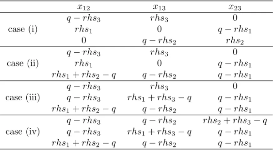
x12 x13 x23 case (i) q−rhs3 rhs3 0 rhs1 0 q−rhs1 0 q−rhs2 rhs2 case (ii) q−rhs3 rhs3 0 rhs1 0 q−rhs1 rhs1+rhs2−q q−rhs2 q−rhs1 case (iii) q−rhs3 rhs3 0 q−rhs3 rhs1+rhs3−q q−rhs1 rhs1+rhs2−q q−rhs2 q−rhs1 case (iv) q−rhs3 q−rhs2 rhs2+rhs3−q q−rhs3 rhs1+rhs3−q q−rhs1 rhs1+rhs2−q q−rhs2 q−rhs1
Table 1: Affinely independent vectors for Theorem 11.
condition 3 is not satisfied. Then, there exists robust cutset inequalityisuch thatrhsi≥q. Hence,
the robust 3-partition inequality is dominated by the robust cutset inequalityi.
Sufficiency. We suppose without loss of generality thatrhs1≥rhs2≥rhs3. According to the values
ofqandrhsifori= 1, . . .3, we distinguish four case: (i)q≥rhs1+rhs2≥rhs1+rhs3≥rhs2+rhs3;
(ii)rhs1+rhs2> q≥rhs1+rhs3≥rhs2+rhs3; (iii)rhs1+rhs2≥rhs1+rhs3> q≥rhs2+rhs3;
(iv)rhs1+rhs2≥rhs1+rhs3≥rhs2+rhs3> q. For each case we provide in Table 4.3 three affinely
independent vectors that are feasible for the problem and satisfy the robust 3-partition inequality with equality. Since the dynamic problem on 3 nodes has the robust cut property [34], the feasibility of a solution can be tested checking the robust cutset inequalities only. It is easy to see that for each case the listed vectors satisfy the robust cutset inequalities. Moreover, one readily verifies that Conditions 1–3 imply that the four 3×3 matrices from Table 4.3 are non-singular.
Therefore, we can prove what follows.
Corollary 12. Inequalities (19)corresponding to connected partitions [S1:S2:S3] that satisfy the
conditions of Theorem 11 are facet-defining forBdynI (spl). Proof. The result follows from Theorems 7 and 11.
We provide next an example of robust 3-partition inequality that satisfies the conditions of Theo-rem 11, but it is not facet-defining for static routing, not even for the budgeted uncertainty set.
Example 13. Consider a complete undirected graph with 3 nodes and let U =Ub. Let the nominal
demands be d¯12 = ¯d13 = 1, d¯23 = 0, the deviations be dˆ12= ˆd13 = 1,dˆ23 = 0, and let Γ = 1. The
robust cutset inequalities and the corresponding robust 3-partition inequality are reported below.
c1: x12+x13≥3
c2: x12+x23≥2
c3: x13+x23≥2
3p: x12+x13+x23≥4
The conditions of Theorem 11 are satisfied, but it is not possible to find three affinely independent integer vectors in 3Bstat
I (spl) that satisfy 3p with equality. In fact, the only capacity allocation
x∈3Bstat
I (spl)that satisfies 3pwith equality is x12=x13= 2,x23= 0.
One can construct similar examples for 3Bvol
I (spl) and 3B af f
I (spl), using the property that affine
routing reduces to static routing whenever the uncertainty set contains the corner of R|+K| [44].
Example 14. Consider the problem in Example 13 and assume that the routing is dynamic, but the flows are unsplittable. The uncertainty set includes traffic matrices A and B, wheredA12= 2,dA13= 1,
dB12= 1,dB13= 2,dA23=dB23= 0. The only solution of value 4 that allows an unsplittable routing for
both AandB isx12=x13= 2,x23= 0.
By Theorem 6, if the robust 3-partitions are not facets for the dynamic problem, they cannot be facets for the static, affine or volume problem under unplittable flows. Indeed, the 3-partitions are not even facets for the deterministic problem, when the flows are unsplittable.
Example 15. Consider a complete undirected graph with 3 nodes and demands d12 = d23 =
0.4, d13= 0.7. Cutset and three-partition inequalities are:
c1: x12+x13≥2
c2: x12+x23≥1
c3: x13+x23≥2
3p: x12+x13+x23≥3
The only unsplittable solution of value 3 is x12=x13=x23= 1, then 3p is not a facet.
We remark again the all the results in Section 4 are independent of the uncertainty setU. Moreover, any inequality that is valid for the capacity formulation is also valid for the flow formulation of the corresponding problem.
5
Test-bed and implementation
Now we consider the Benders formulations from a computational perspective. We restrict to splittable flows and toUb. The purpose of the computational experiments presented in this section is two-fold.
First, we test the solvability of the Robust Network Loading Problem using different formulations and settings, on real-life instances. The scope is to show which are the approaches that can be used on problems coming from real applications and which are the approaches that are computationally problematic on such instances. Second, we compare the optimal solution values on both realistic instances and randomly generated ones. Let opt(r) denote the optimal solution of the problem when routing policyr is considered. Then, we see immediately that the following ordering holds:
opt(dyn)≤opt(af f)≤opt(vol)≤opt(stat).
Our purpose is to show the trade-off between the value of the produced solution (flexibility) and the required time.
5.1
The test-bed
Our test bed contains two classes of instances, that we denote byrealisticandrandom. The first class of instances includes 12 realistic network instances available from SNDlib [39]. Networks abilene, germany, andgeant come from [26], where the authors build nominal demand values and deviations according to historical traffic data. Notice that our instances may differ slightly from the instances from [26], because we kept only commodities whose nominal demand value was greater than 0.001, to avoid numerical issues. For the other seven networks, we define the nominal demand value as the deterministic one and let the deviation be 50% of the nominal demand, as in [8, 44]. The purpose of the realistic instances is to test the performances of the different approaches on real-life instances. The second class of instances includes 12 randomly generated instances. Networks are randomly generated so that each node has at least two incoming edges to avoid trivial problems. Demands are computed generating random numbers is [1,9] and then dividing them by 10. Edge costs are randomly generated integer numbers in{1, . . . ,5}. The purpose of the random instances is to provide instances that can be solved to optimality by all the approaches to compare the corresponding costs, without being possibly biased by the unsolved instances. Hence, they are much easier to solve than the realistic instances, with minimal differences in the computing times depending on the routing
policy.
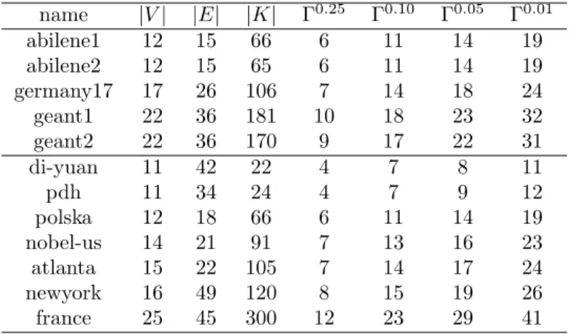
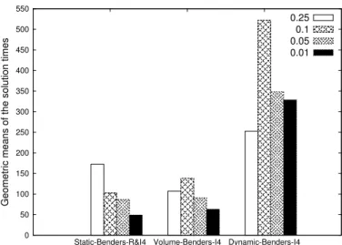
We choose the value of Γ according to the probabilistic bound introduced in [15]. Namely, we set four levels of guaranteed probabilistic bound (denoted ): 0.25,0.10,0.05,and 0.01. Then, for each value of , the corresponding Γ is such that all feasible solutions for the dynamic and the affine problem satisfy the following property: if demands are symmetric and independent random variables distributed in [ ¯d−d,ˆd¯+ ˆd], then, for eacha∈A, the probability that the flow exceeds the capacity installed on arcais less than. In this way we obtain 48 instances for the realistic instances and 48 instances for the random instances. A description of the realistic instances is reported in Table 2, while Table 3 refers to the random instances.
name |V| |E| |K| Γ0.25 Γ0.10 Γ0.05 Γ0.01 abilene1 12 15 66 6 11 14 19 abilene2 12 15 65 6 11 14 19 germany17 17 26 106 7 14 18 24 geant1 22 36 181 10 18 23 32 geant2 22 36 170 9 17 22 31 di-yuan 11 42 22 4 7 8 11 pdh 11 34 24 4 7 9 12 polska 12 18 66 6 11 14 19 nobel-us 14 21 91 7 13 16 23 atlanta 15 22 105 7 14 17 24 newyork 16 49 120 8 15 19 26 france 25 45 300 12 23 29 41
Table 2: Realistic instances description
name |V| |E| |K| Γ0.25 Γ0.10 Γ0.05 Γ0.01 n10e14d14 1 10 14 14 3 6 7 10 n10e14d14 2 10 14 14 3 6 7 10 n10e14d14 3 10 14 14 3 6 7 10 n10e14d19 1 10 14 19 4 6 8 11 n10e14d19 2 10 14 19 4 6 8 11 n10e14d19 3 10 14 19 4 6 8 11 n10e19d14 1 10 19 14 3 6 7 10 n10e19d14 2 10 19 14 3 6 7 10 n10e19d14 3 10 19 14 3 6 7 10 n10e19d19 1 10 19 19 4 6 8 11 n10e19d19 2 10 19 19 4 6 8 11 n10e19d19 3 10 19 19 4 6 8 11
Table 3: Random instances description
5.2
Implementation
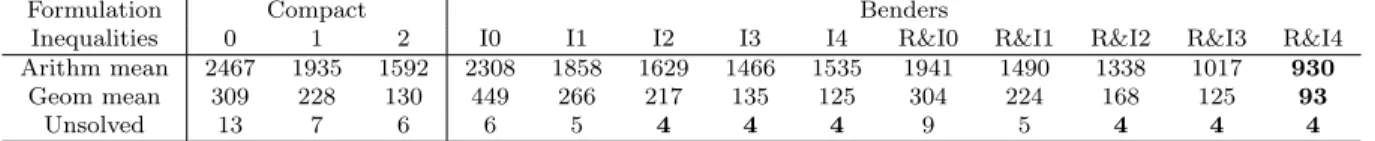
The solution approaches have been coded in JAVA using Cplex Concert Technology using default cut generation parameters. All computations were run on a computer equipped with an Intel(R) Xeon(R) CPU E5540 2.53GHz processor and 16 GB of RAM, using CPLEX 12.6 [21]. We allow 7200 seconds of computing time for each instance. For the affine and the dynamic problem only the Benders formulation is considered. For the static and the volume problem, two approaches are used. The first approach solves the compact formulations f V RN L andf SRN L, enhanced by the separation of robust cutset and robust 3-partition inequalities at the root node. The second approach addresses the problems via a Benders decomposition algorithm. The algorithm starts with a master
problem that contains one robust cutset inequality for each node of the network, then the problem is solved by branch-and-cut generating robust cutset, robust 3-partition and Benders inequalities according to the considered setting. In the following, we refer shortly to these two approaches as Compact and Benders, respectively. Then, the Benders inequalities are generated at each integer solution and, possibly, at the root node on any solution. We generate robust cutset and 3-partition inequalities, according to one of the following configurations:
0 : No cuts.
1 : Heuristic and exact separation of robust cutset inequalities at the root node only.
2 : 1+ heuristic separation of robust 3-partition inequalities at the root node only.
3 : Heuristic and exact separation of robust cutset inequalities at the root node and at integer solutions.
4 : 3+ heuristic separation of robust 3-partition inequalities at the root node and at integer solutions. Notice that for the Compact formulation approach, only the first three implementations are tested. We also test whether it is better to generate Benders inequalities only at integer solutions (I) or at integer solutions and at the root node (R&I). Hence, we compare 10 approaches for Benders decomposition: R&I and I for eachm∈ {0,1,2,3,4}. For each of these configuration, the inequalities are separated in this order: 1) heuristic separation of robust cutset inequalities, 2) heuristic separation of robust 3-partition inequalities, 3) exact separation of robust cutset inequalities, 4) separation of Benders inequalities (only for Benders decomposition approaches). The problems are solved by a branch-and-cut algorithm, both for the Compact and for the Benders approach. That is, instead of solving the Benders master problem to integrality at every iteration as in [27], we solve the linear relaxation, as in a traditional branch-and-cut framework. This approach is known to yield much faster algorithms (see for example [24]). As soon as an inequality is found violated, the other inequalities are skipped and the linear programming relaxation is solved again. Another important characteristic of the Benders decomposition algorithm is the primal heuristic provided at the root node. Namely, the linear programming relaxation is first solved for the static problem using the compact formulation and the resulting capacities are rounded up to the nearest integer values. Although negligible, the solution time of this heuristic is included in the total solution time. We also tried, in some preliminary computations, the automatic Benders decomposition of CPLEX 12.7, but our ad-hoc approach turned out to have better performances.
Separation of robust cutset inequalities When the budgeted uncertainty set is used, the robust
cutset inequalities are rewritten as:
X e∈E(S1,S2) xe≥ X k∈K(S1,S2) ¯ dk+ max Q⊆K(S1,S2),|Q|≤Γ X k∈Q ˆ dk .
We separate them using two approaches. The first approach separates the cut heuristically as follows. We randomly partition the nodes into two subsets and then perform a local search picking up one node and moving it to the other subset, until there is no more improvement in the violation. If no violated inequality has been found, we choose another partition, up to a maximum of 5 iterations. The second approach separates the inequalities exactly through the following formulation.
max −X e∈E xeµe+β s.t. µe≥max{ri−rj, rj−ri} e∈E (20a) µe≤min{ri+rj,2−rj−ri} e∈E (20b) νk ≥max{rsk−rtk, rtk−rsk} k∈K (20c) νk ≤min{rsk+rtk,2−rsk−rtk} k∈K (20d)
`k ≤min{γk, νk} k∈K (20e) β≤ X k∈K ¯ dkνk+ X k∈K ˆ dk`k+ 1− (20f) X k∈K γk = Γ γ,`∈ {0,1}|K|,µ∈ {0,1}|E|,ν∈ {0,1}|K| β∈Z,r∈ {0,1}|V|
Variable ri is one if node i belongs to set S of the partition and zero otherwise. Variable `k and
constraints (20e) represent product γkµk. Constraints (20a)–(20d) ensure that µe (resp. νk) are
equal to one if and only if the endpoints of the edge (resp. commodity) belong to different subsets of the partition. We remind that the robust cutset inequalities belong to the first Chv´atal closure and, under some assumptions, they are facets of the problem for all the considered routing policies.
Separation of robust 3-partition inequalities We separate the robust 3-partition inequalities
heuristically as follows. We randomly partition the nodes into three subsets and then perform a local search picking one node and moving it to another subset, until there is no more improvement in the violation. If no violated inequality has been found, we choose another partition, up to a maximum of 5 re-starts. Is is also possible to develop an exact algorithm based on a generalization of formulation (20). We have a set of variables and constraints for every cut, plus extra binary variablesηand integer Θ representing the 3-partition and the right-and-side of the inequality, to be computed rounding the right-hand-sides of the robust cutset inequalities. However, a preliminary testing proved this formulation to be quite slow in practice, therefore we rely on the heuristic approach, as usually done in the literature for partition-based inequalities other than cutsets, even for the problem without uncertainty [1]. We remark that the robust 3-partition inequalities are facets under some conditions of the problem with dynamic routing, while they belong to the second Chv´atal closure for the other routing schemes, as they are obtained combining the robust cutset inequalities, that belong to the first Chv´atal closure.
Separation of Benders inequalities Benders inequalities are separated exactly by solving
prob-lems (11) and (16), depending on the routing scheme. After finding a violated inequalityµTx≥b, its coefficients and right-hand-side are rounded using the following approach, originally proposed in [16]. It consists of replacing the inequality by
X e∈E µ e µmin xe≥ b µmin ,
whereµminis the smallest positive entry ofµ. In the unlikely situation where the rounded cut is not
violated, instead, we add the original cut. We note that one could directly separate inequalities with integer µ and b being the upper integer of the corresponding Benders cut (also known as rounded metric inequalities). However, a preliminary testing proved that separating Benders inequalities in their non-rounded form and then strengthening them, is computationally more efficient than solving the integer separation problem. We note that the strengthened Benders cuts we use here belong to the first Chv´atal closure, as they are obtained (heuristically) rounding a single inequality of the formulation.
6
Results
This section is organized as follows. First we discuss the information obtained about the costs corresponding to the different routing schemes using the random instances, then we analyze in detail the results obtained on the realistic instances.
Solution costs Best solution time/Best gap name 1− optstat redvol(%) redaf f(%) reddyn(%) stat vol af f dyn
abilene1 0.25 31 0.0 0.0 0.0 1 3 2416 8 0.1 32 0.0 0.0 0.0 1 3 1379 13 0.05 33 0.0 0.0 0.0 2 3 1532 5 0.01 33 0.0 0.0 0.0 1 4 1780 3 abilene2 0.25 20 5.0 5.0 5.0 2 2 1568 16 0.1 22 0.0 0.0 0.0 2 3 3986 7 0.05 22 0.0 0.0 0.0 1 2 1838 3 0.01 22 0.0 0.0 0.0 1 3 1686 3 germany17 0.25 35 2.9 ≥0.0 2.9 65 12 28% 54 0.1 36 0.0 0.0 0.0 7 20 27% 32 0.05 36 0.0 0.0 0.0 8 14 28% 932 0.01 36 0.0 0.0 0.0 7 10 26% 13 geant1 0.25 30 0.0 0.0 0.0 72 142 M 2551 0.1 31 3.2 ≥0.0 ≥0.0 1849 138 M 35% 0.05 31 3.2 ≥0.0 ≥0.0 200 142 M 33% 0.01 31 0.0 ≥0.0 ≥0.0 78 65 M 22% geant2 0.25 34 2.9 ≥0.0 2.9 662 134 M 837 0.1 34 0.0 ≥0.0 ≥0.0 72 53 M 18% 0.05 34 0.0 ≥0.0 ≥0.0 79 126 M 36% 0.01 34 0.0 ≥0.0 ≥0.0 343 93 M 15% di-yuan 0.25 5240900 8.5 9.6 9.6 79 6 118 4 0.1 5366800 1.9 3.6 3.7 8 119 1697 17 0.05 5371400 1.1 2.6 2.8 6 32 5390 6 0.01 5371400 0.0 0.0 0.0 1 2 96 1 pdh 0.25 850604.8 4.8 6.2 6.5 279 282 4202 12 0.1 852303.1 0.1 0.0 0.6 41 149 1% 15 0.05 852585.8 0.0 0.0 0.1 8 22 1558 3 0.01 853009.8 0.0 0.0 0.0 6 10 913 3 polska 0.25 261.2 12.4 ≥0.0 ≥0.0 21 44 18% 18% 0.1 287.4 12.8 ≥9.3 ≥0.0 31 17 20% 19% 0.05 293.5 10.9 14.5 ≥0.0 878 95 6337 17% 0.01 295.1 5.1 8.8 ≥0.0 101 28 6329 12% nobel-us 0.25 294886.5 10.5 ≥0.0 ≥0.0 37 266 18% 18% 0.1 315622.5 9.2 ≥0.0 ≥0.0 34 1137 16% 16% 0.05 319814.5 7.9 ≥0.0 ≥0.0 113 324 15% 15% 0.01 322963.5 4.3 ≥0.0 ≥0.0 499 956 12% 12% atlanta 0.25 200105 4.7 ≥0.0 5.4 20 163 11% 1902 0.1 209610 3.4 ≥0.0 ≥0.0 41 74 8% 8% 0.05 211680 2.7 ≥0.0 ≥0.0 130 26 8% 8% 0.01 214480 1.7 ≥0.0 ≥0.0 81 27 6% 6% newyork 0.25 985.2 0.0 0.0 0.0 49 110 82% 22 0.1 985.2 0.0 0.0 0.0 47 140 82% 32 0.05 985.2 0.0 0.0 0.0 51 114 83% 34 0.01 985.2 0.0 0.0 0.0 38 162 83% 20 france 0.25 10.4 7.7 ≥0.0 ≥0.0 4074 2196 M 20% 0.1 11 6.4 ≥0.0 ≥0.0 678 4136 M 21% 0.05 11.2 5.4 ≥0.0 ≥0.0 599 3961 M 73% 0.01 11.5 4.3 ≥0.0 ≥0.0 1% 1% M 19%
0 1 2 3 4 5 6 7 8 0.25 0.1 0.05 0.01
Arithmetic means of the cost reductions (\%)
volume affine dynamic (a) Varying. 0 1 2 3 4 5 14 19
Arithmetic means of the cost reductions (\%)
volume affine dynamic (b) Varying|K|. 0 0.5 1 1.5 2 2.5 3 3.5 4 14 19
Arithmetic means of the cost reductions (\%)
volume affine dynamic
(c) Varying|E|.
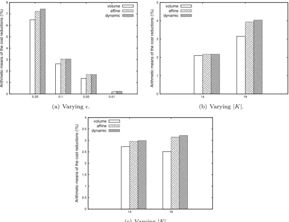
Figure 1: Cost reductions from the static routing solution on the instances from Table 3.
Random instances The purpose of the experiments here is to compare the costs associated with
the different routing policies. In order to do that, we compare the objective values obtained solving the problem corresponding to each routing policy. Hence, as said above, these instances are generally much easier to solve than the realistic instances, with no relevant differences between the routing policies. We present in Figure 1 the average cost reductions over static routing for the instances described in Table 3. Globally, the results show that the cost reductions obtained for volume and affine routing are close to those obtained for dynamic routing. In addition, Figure 1(a) highlights that decreasing the value of(i.e. increasing the value of Γ) reduces significantly all cost reductions, while Figure 1(b) illustrates how increasing the number of commodities increases all cost reductions. Regarding the number of edges of the network, Figure 1(b) shows that networks with more edges yield a slight increase in the cost reduction obtained by affine and dynamic routing while the opposite holds for volume routing.
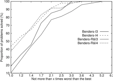
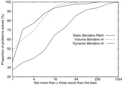
Outline of the results on realistic instances We present first an overview of the results,
paying a particular attention to the cost reductions offered by volume and dynamic routing. Then, we compare the efficiency of the different algorithms for solving each type of routing, but affine routing, where our approach could solve only one third of the instances. This step is carried out by comparing the arithmetic and the geometric means of the solution times and the number of unsolved instances. It is worth recalling that the arithmetic mean gives more weight to hard instances, while the geometric mean considers equally all instances, regardless of their difficulty. Notice also that this approach hides a part of the difficulty of the unsolved instances, since their solution times count for 7200 seconds in all computations. Hence, we report actual lower bounds for the true (unknown) means. This comment is particularly important for dynamic routing, for which some instances could not be solved. In spite of this, these aggregated results give us valuable insight for choosing the approach that seems the best for each routing. After studying each routing individually, we compare