Educational Implications of School Systems at Different Stages of Schooling
43
0
0
Full text
(2) Educational Implications of School Systems at Different Stages of Schooling. Jung Hur. Changhui Kang*. Department of Economics National University of Singapore. Abstract In educating students national public school systems use different methods of grouping students by ability across schools. We consider four different school systems of student allocation at different stages of schooling and their educational implications. Our twoperiod model suggests that both the frequency and sequence of ability grouping play an important role in producing educational implications. As different households prefer different combinations of school systems, the overall performance of a school system is determined by how households are distributed over income and a child's ability and the voting of households.. Key Words: Education, Comprehensive and Selective School Systems JEL Classification: D11, I20. *. Corresponding author: Changhui Kang, Address: Department of Economics, National University of Singapore, AS2 1 Arts Link, Singapore 117570, Singapore, Email: [email protected], Tel: +65-65166830, Fax: +65-6775-2646..
(3) Educational Implications of School Systems at Different Stages of Schooling. In educating students national public school systems use different methods of grouping students by ability across schools. We consider four different school systems of student allocation at different stages of schooling and their educational implications. Our twoperiod model suggests that both the frequency and sequence of ability grouping play an important role in producing educational implications. As different households prefer different combinations of school systems, the overall performance of a school system is determined by how households are distributed over income and a child's ability and the voting of households. Key Words: Education, Comprehensive and Selective School Systems JEL Classification: D11, I20. 1. Introduction In educating students national public school systems around the globe use different methods of grouping (or ungrouping) students by ability across schools. Some countries such as Germany, pre-1960s U.K., China and Singapore adopt selective systems based on school entrance exams to place students to schools; other countries such as U.S., contemporary U.K. and South Korea employ comprehensive systems based on residential school districts to allocate students. Within the group of countries that rely on selective systems, the starting point of ability grouping across schools varies in the procession of schooling, although most countries adopt mixed-ability schooling in an early part of primary education. For example, Germany first divides different-ability children into different school tracks (Gymnasium, Realschule and Hauptschule) at age 10; prior to school reforms in 1960s U.K. placed children to different types of schools according to ability (grammar and secondary modern schools) at age 11; China and Singapore send primary-school graduates to ability-stratified secondary schools at age 13; Japan employs similar grouping at age 16. In contrast, such ability grouping across schools does not exist in countries that in principle adopt comprehensive systems of public primary and secondary education, although ability-tracking within mixed-ability schools is exercised in some cases (e.g., U.S.; rare in South Korea). Despite the heated debates for last decades as to whether to group students by ability and from when to group them, educational experts and parents have yet to reach consensus on these issues. Proponents of comprehensive systems argue that the major 1.
(4) objective of a school system is to provide equal educational opportunities to all students irrespective of family and social backgrounds. They contend that by giving students rights to attend any school in the neighborhood, education can serve as a method for narrowing educational inequality (Jenkins et al., forthcoming; Leschinsky and Mayer, 1990; Oakes, 1985). In contrast, advocates of selective systems argue that selective schooling maximizes educational outcomes because it is easier for teachers to instruct groups of students with a low variance of ability and for students to learn with similarability students in school (Gamoran, 1986; Lazear, 2001). They also believe that a selective system is more fair since student allocation is based upon ability alone, not upon family background.1 In contrast to grown interests in school systems of student allocation, economic studies of education are rare that directly deal with educational implications of comprehensive and selective school systems. Even more scarce are studies that examine an optimal timing and sequence of ability grouping across schools in terms of efficient and equitable educational production.2 Nevertheless, there exist four papers that are directly related to school systems. Benabou (1996) examines implications of ability grouping and mixing of students, arguing that ability mixing tends to slow down the short-run growth but raise the longrun growth. Fernandez and Gali (1999) compare the relative performance of markets and tournaments---ability grouping by a test---in an economy with borrowing constraints. They show that tournaments dominate markets in terms of matching efficiency. Lazear (2001) investigates how educational outputs are affected by grouping methods of different-quality students to show that the total educational output is maximized when students are grouped according to quality. Finally, Hur and Kang (2007) rely on a simple economic model for households' choices on consumption and educational investments to explore varying educational implications of comprehensive. 1. Further details on comprehensive and selective schooling and their effects on education are well. surveyed by Gamoran and Mare (1989), Ireson and Hallam (1999), Kerckhoff (1986) and Slavin (1987, 1990) among others. 2. This situation is a little surprising given that such issues are under continuing discussions in many. countries, and often more emphasized outside North America than school resource effectiveness (e.g., Hanushek and Woessmann, 2006). Recent research in economics of education that shows the presence of positive and nonlinear peer effects in primary and secondary education also underscores the importance of different methods of student grouping in educational production (e.g., Ding and Lehrer, 2007; Kang, 2007).. 2.
(5) and selective school systems for efficiency and equity of education. All these studies are, however, completely silent about when it is optimal to start ability grouping across schools to achieve educational goals of a society.3 For want of relevant studies, the current paper examines two issues that are of primary concern in the construction of school systems: whether and when to group students by ability across schools. Given that there are in general two stages of public schooling---primary and secondary levels---that produce the ultimate educational outcome, we investigate whether it is desirable to adopt ability grouping and when it is optimal to start (or not start) such grouping in order to achieve often-conflicting educational goals of efficiency and equity.4 To this end, we extend Hur and Kang's (2007) one-period model to the case where the decisions are made in two periods reflecting two stages of public education before college. In the analysis each of comprehensive and selective systems is characterized by the role of a student's own quality prior to school entrance and the parent's choice of residential district in the determination of quality of school peers. We then compare efficiency and equity of educational outcomes across different school systems by examining educational expenditures, the role of family income and student ability in the determination of the educational outcome, and the variance and level of such an outcome. Our two-period model of school systems gives rise to several points that have failed to emerge in previous discussions on school systems. Above all, it suggests that not only the frequency of ability grouping in two stages of schooling but its sequence also matter in drawing educational implications of school systems. Given that there are two methods of grouping students (comprehensive and selective) and two stages of schooling (primary and secondary), we have four different school systems to use in educating students: (1) the comprehensive-comprehensive (CC) system in which the comprehensive system is employed in stage 1 (e.g., primary level) and stage 2 (e.g., secondary level) alike; (2) the selective-selective (SS) system in which the selective. 3. See Hur and Kang (2007) for further theoretical discussions on these four papers and empirical findings. about the effects of comprehensive and selective systems on efficiency and equity of education. 4. In this paper our primary concern is about how to allocate students across schools, not across classes. within a school given that the students are already placed to the school. For issues and impacts of withinschool ability grouping and mixing on education, see, e.g., Argys et al. (1996), Betts and Shkolnik (2000), Figlio and Page (2002), Gamoran (1987), and Slavin (1990). In addition, we focus exclusively on public school systems, ignoring the presence of private schools. For issues concerning the role of ability grouping in the relationship between public and private schools, see, e.g., Epple et al. (2002).. 3.
(6) system is adopted in both stages; (3) the comprehensive-selective (CS) system in which the comprehensive (selective) system is used in stage 1 (stage 2); (4) the selectivecomprehensive (SC) system in which the selective (comprehensive) system is used in stage 1 (stage 2). The first three systems (i.e., CC, SS and CS) are often observed in existing educational institutions. However, the SC system is hard to find. Below we show that the SC system at times reveals more desirable educational implications than the CC and CS systems. Thus the sequence of ability grouping can make differences in achieving educational goals. Second, we find that different households that are characterized by a pair of family income and the child's innate ability prefer different combinations of school systems. For example, households in which the income is high but the child's ability is low tend to like CC but dislike SS; households in which the income is high and the child's ability is also high tend to like CS but dislike SC; and so on. Thus the overall performance of a school system is determined by how households are distributed over income and child ability and how they prefer each school system. Which sequence of school systems is adopted in a nation's education system will be ultimately determined by voting of households. Third, if the entrance exam in the selective system tests a student's endowed ability alone but never her nurtured ability, then the systems that adopt the selective method in the later stage of education show more favorable educational implications than if the exam tests a student's endowed ability as well as her nurtured ability. Whether or not the entrance exam should signal the endowed ability alone in the selective system will also be determined by voting of households, because different households prefer different settings of the entrance exam in the selective system. The rest of the paper proceeds as follows: section 2 extends Hur and Kang's (2007) one-period model to a two-period case in which comprehensive and selective systems are combined with different sequences. In section 3 we discuss analytical results of the four school systems in terms of efficiency and equity of education. Section 4 introduces a new setting of the entrance exam in the selective system and examines its educational implications under the four systems. Section 5 concludes the paper. 2. The model Let us first set up a utility function of a household that consists of a parent and one child:. 4.
(7) U = ln U 1 + ρ ln U 2. (1). where U t = xtα At = xtα ( At −1θ tβ etγ ) , α + β + γ = 1 , 0 < α , β , γ , ρ < 1 , and t = 1, 2 .5. Here the household's total utility ( U ) is expressed by a sum (in natural log) of period-1 utility ( U 1 ) and period-2 utility ( U 2 ) that is discounted by a factor ρ . A period- t utility is determined by the amount of private goods consumption ( xt ) and the child's educational outcome ( At ) at period t . The educational outcome at t is produced by the child's educational outcome in the previous period ( At −1 ), the average quality of peers in school ( θ t ), and the amount of private educational services ( et ) that can be purchased in a form of private tutoring in the market. 6 The child's timeinvariance ability endowed from birth is denoted by A0 . Now we consider two major school systems that exist in public primary and secondary education: comprehensive and selective school systems. At each stage of schooling, the comprehensive system is characterized by school districts based on residential location. In this system parents choose a school district and their children are placed into one school within the school district. In contrast, the selective system is characterized by entrance tests. In this system students take an entrance exam and are admitted to a school according to their ranking in the exam. In our analysis of comprehensive systems, we suppose, for simplicity, that student placement into a school is random within a school district, while parents can freely choose the school district.7 We also assume that there is a fixed number of school. 5. The current Cobb-Douglas form of utility and educational production functions plays an important role. in drawing differences in educational implications across different school systems in this paper. However, the adoption of such a functional form is not unique to the current study. They are often employed by the economics of education literature (e.g., Epple et al., 2002; Epple and Romano, 1998; Ferreyra, forthcoming; Lazear, 2001; Nechyba, 2000). See Hur and Kang (2007) for further discussions on alternative functional forms. 6. To focus exclusively on the impacts of student allocation across schools, we assume that every public. school spends an equal amount of resources for a student, setting monetary resource allocation across schools and districts aside. For issues related to school financing and the distribution of the resources, see, e.g., Fernandez and Rogerson (2003) and Hoxby (2001). 7. Under comprehensive systems, there are largely two methods of student placement within a school. district. The first is to assign each student randomly to one school within the district. This method has been employed in South Korea since 1969 to allocate students to middle schools and general (or nonvocational) high schools within a school district. See OECD (1998, Chapters 1 and 2) for details. The. 5.
(8) districts to serve entire population of students, and that each district is identical in terms of the number of schools and school resources such as class size, teacher quality, etc. Under the comprehensive system, the quality of school peers ( θ t ) is exogenously given to individual students once a school district is decided: within a district, students face the same average quality of peers in any school due to randomization. Nonetheless, parents may choose the quality of school peers indirectly by moving across school districts. The children's quality of a school district is reflected in house prices (Black, 1999; Gibbons and Machin, 2003). Let us denote the children's average quality of a school district by d t and its unit price by p dt . Parents spend a total of p dt d t to purchase a house in a certain school district; a high house price in a good school district is expressed by a high value of d t , hence p dt d t . In the model, for simplicity again, we suppose that there are no commuting costs between the house and school, and no changes in living environment over time. In contrast to comprehensive systems, the choice of a school district does not matter in the determination of school peer quality under selective systems, because schools give admissions to students based on the entrance exam ranking alone, not on the school district. Note that the total number of schools and school resources remain unchanged compared with those of the comprehensive system; only school districts disappear in the selective system. In this system parents choose the quality of school peers solely by raising the entrance exam ranking of the child; the quality of school peers ( θ t ) is determined by the child's own quality at the end of the previous period ( At −1 ). That is, the level of θ 1 is decided by that of A0 ---the endowed quality---and the level of θ 2 by that of A1 ---the endowed plus nurtured quality just prior to period 2.8 To characterize different systems of student allocation to schools at t , we introduce the following model for θ t :. second is to assign each student to one school within a district in consideration of the preferences of the student and parent. Such a method is more common in comprehensive systems than random assignment. In our analysis, however, we assume random assignment within a district for conceptual sharpness. 8. In section 4 we analyze educational implications of selective school systems where the entrance exam. tests a student's endowed ability A0 alone (not At −1 ) at each stage of schooling, and compare them with those obtained in the current setting of the entrance exam. An interesting result is that inequality of the educational outcome under selective systems is reduced in the system relying on A0 relative to the system relying on At −1 . Details are presented in section 4.. 6.
(9) θ t = Atτ−1 d tδ t. for t = 1, 2. t. (2). The comprehensive system is characterized by τ t = 0 and δ t = 1 , and the selective system by τ t = 1 and δ t = 0 . δ t is equal to one in the comprehensive system that employs within-district randomization, because θ t , the average peer quality in a school, is ultimately determined by d t , the average quality of children in a school district.9 For the selective system we assume that τ t = 1 for simplicity of analysis. Namely, in the selective system the average quality of school peers is equal to a student's own quality. If either τ t > 1 or 0 < τ t < 1 , then student allocation is infeasible given a pool of students to be assigned to schools.10 In sum, a household's utility function at t is denoted by: U t = xtα At = xtα { At −1 ( Atτ−t 1 d tδ t ) β etγ } = xtα ( At1−+1τ t β d tδ t β etγ ) 9. If a within-district allocation of students is not random, then. 10. The assumption that. τt =1. δt. (4). may deviate from one.. in the selective system holds strictly only in a very restrictive condition. that students in a given school have the same value of At −1 . For illustration, suppose that there are a total of 100 students to be placed to a total of 10 schools in the selective system. Suppose also that the best 10 students score 10 in the exam that determines At −1 ; the second best 10 students score 9; the third best 10 students score 8; and so on. In such a case the best school (say, school 1) is attended by the best 10 students with an identical score 10; the second best school (say, school 2) by the second best 10 students with score 9; and so on. Each school is attended by students with the same value of At −1 . In this case alone. θt. is exactly equal to At −1 , hence. At −1 can be described by a discrete step. τ t = 1 ; the entire functional relationship between θ t and function whereby the value of θ t jumps up by 1 as At −1. rises by 1. In more realistic cases where individual students have different (continuous) scores of At −1 , the exact relationship between. θt. and At −1 will also be a similar step function; the difference,. however, is that within a given school. θt. falls as At −1 rises, because. θt. is determined by the. average value of At −1 among the schoolmates excluding the self. There is a jump in. θt. across. different schools as At −1 rises. Such a step function can be approximated by a linear function with slope 1, i.e.,. θ t = At −1 .. We use such an approximation to characterize the selective system. Given the. approximated formula, there is likely to exist a deviation of. θt. from At −1 for an individual student in. more realistic cases; it will not be large, however, in the selective system because a school is attended by students with similar At −1 . In our presentation we sacrifice mathematical rigor of the relation between. θt. and At −1 for conceptual sharpness of the subsequent analysis but the cost does not seem to be. terribly large.. 7.
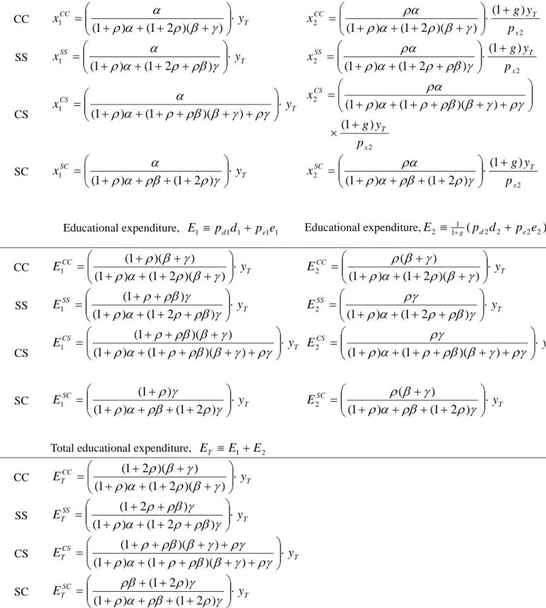
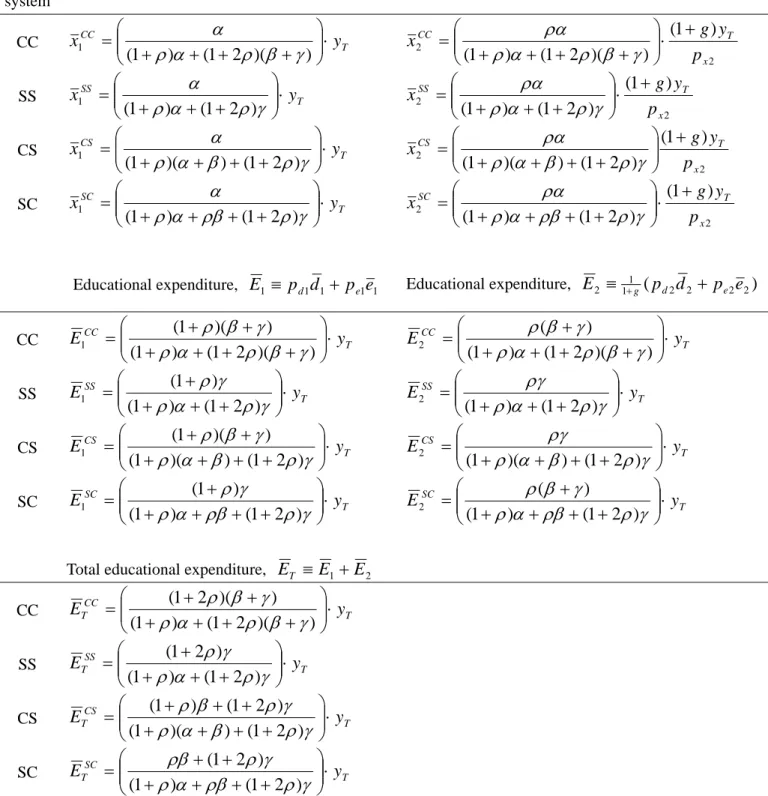
(10) And the total utility is given by: U = α [ln x1 + ρ ln x2 ] + (1 + ρ + ρβτ 2 )[(1 + βτ 1 ) ln A0 + βδ 1 ln d1 + γ ln e1 ] + ρ [ βδ 2 ln d 2 + γ ln e2 ]. (5). Now consider the household's budget constraint:. x1 + p d 1 d1 + p e1e1 +. y 1 ( p x 2 x 2 + p d 2 d 2 + p e 2 e2 ) ≤ y1 + 2 ≡ yT 1+ g 1+ g. (6). where y t is the post-tax disposable income of the household at t , yT is its total present-value disposable income, and g is the interest rate of the private credit market. The price of x1 is assumed to be one for normalization. All the prices are exogenously determined in their own perfectly competitive markets. Subject to the budget constraint, the household, which is uniquely characterized by a pre-determined set of A0 , y1 and y 2 , chooses the total utility maximizing levels of x1 , x 2 , e1 and e2 together with. those of d 1 and d 2 the choices of which depend on the school system adopted. The optimal quantities of the choice variables, the educational outcome and indirect utilities are obtained as following: ⎞ ⎛ α ⎟⎟ ⋅ yT x1* = ⎜⎜ ⎝ (1 + ρ )α + (1 + ρ + ρβτ 2 )( βδ 1 + γ ) + ρ ( βδ 2 + γ ) ⎠. (7). ⎞ yT ⎛ (1 + ρ + ρβτ 2 ) ⋅ βδ 1 ⎟⎟ ⋅ d1* = ⎜⎜ ⎝ (1 + ρ )α + (1 + ρ + ρβτ 2 )( βδ 1 + γ ) + ρ ( βδ 2 + γ ) ⎠ p d 1. (8). ⎞ yT ⎛ (1 + ρ + ρβτ 2 ) ⋅ γ ⎟⎟ ⋅ e1* = ⎜⎜ ⎝ (1 + ρ )α + (1 + ρ + ρβτ 2 )( βδ 1 + γ ) + ρ ( βδ 2 + γ ) ⎠ p e1. (9). ⎞ (1 + g ) yT ⎛ ρα ⎟⎟ ⋅ x 2* = ⎜⎜ px2 ⎝ (1 + ρ )α + (1 + ρ + ρβτ 2 )( βδ 1 + γ ) + ρ ( βδ 2 + γ ) ⎠. (10). ⎞ (1 + g ) yT ⎛ ρβδ 2 ⎟⎟ ⋅ d 2* = ⎜⎜ pd 2 ⎝ (1 + ρ )α + (1 + ρ + ρβτ 2 )( βδ 1 + γ ) + ρ ( βδ 2 + γ ) ⎠. (11). 8.
(11) ⎛ ⎞ (1 + g ) yT ργ ⎟⎟ ⋅ e2* = ⎜⎜ pe2 ⎝ (1 + ρ )α + (1 + ρ + ρβτ 2 )( βδ 1 + γ ) + ρ ( βδ 2 + γ ) ⎠. (12). At* = ( At*−1 )1+τ t β (d t* ) δ t β (et* ) γ. (13). U t* = ( xt* ) α At*. (t = 1, 2). (t = 1, 2). (14). U * = ln U 1* + ρ ln U 2*. (15). Hereafter, we will drop the asterisks of the variables, unless the optimized value may be confused with the variable itself. 3. School Systems and Educational Implications. Now we consider four different school systems of student allocation at different stages of schooling (e.g., primary and secondary education): the comprehensivecomprehensive (CC) system, the selective-selective (SS) system, the comprehensiveselective (CS) system and the selective-comprehensive (SC) system, as defined previously. From the discussions in section 2, the CC system is characterized by τ 1 = τ 2 = 0 and δ 1 = δ 2 = 1 ; the SS system by τ 1 = τ 2 = 1 and δ 1 = δ 2 = 0 ; the CS system by τ 1 = 0 , τ 2 = 1 , δ 1 = 1 and δ 2 = 0 ; the SC system by τ 1 = 1 , τ 2 = 0 , δ 1 = 0 and δ 2 = 1 . Given such characterizations of different school systems, we employ a few criteria to compare educational implications across different systems. These criteria include the consumption levels ( xt ), educational expenditures ( Et ≡ p dt d t + p et et ), and the final educational outcome ( A2 ), because they are often examined in theoretical and empirical discussions on school systems (see Hur and Kang (2007) for details). Table 1 summarizes such measures for each school system. From equations (7) to (9) we can show that a household with a pre-determined income schedule ( y1 , y 2 ) reveals saving patterns that vary according to school systems. In general, the optimal amount of period-1 saving of a household with ( y1 , y 2 ) is given by. S1 = y1 − ( x1 + p d 1 d1 + p e1e1 ) =. ρ (α + βδ 2 + γ ) y1 − 1+1g [α + (1 + ρ + ρβτ 2 )( βδ 1 + γ )] y 2 (1 + ρ )α + (1 + ρ + ρβτ 2 )( βδ 1 + γ ) + ρ ( βδ 2 + γ ). 9.
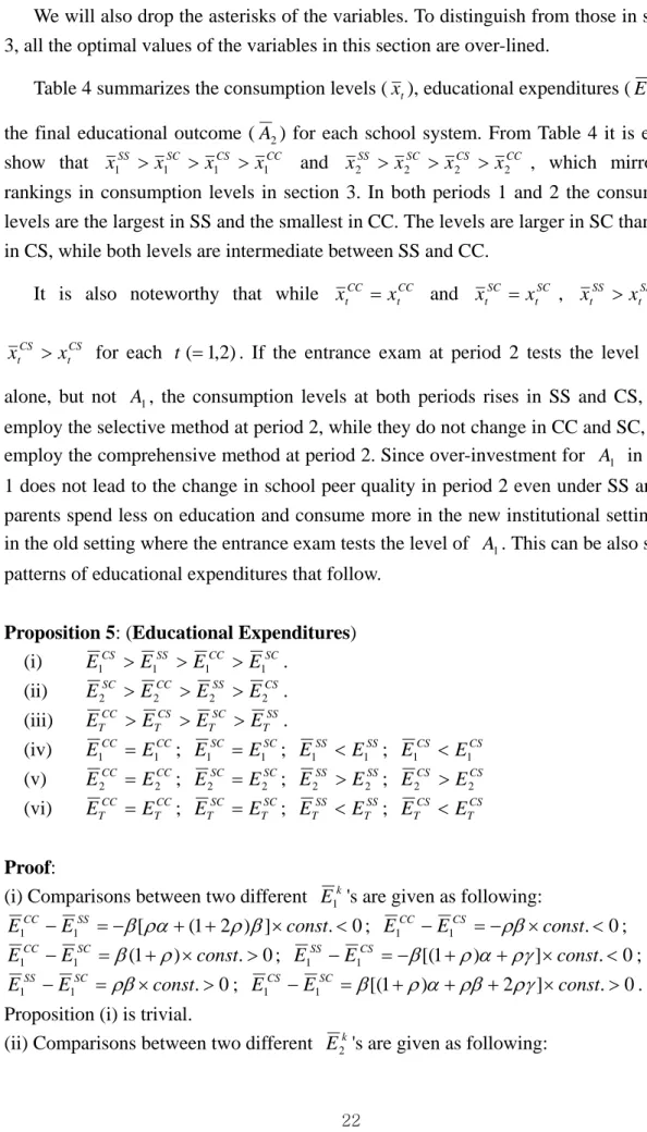
(12) This suggests that the optimal amount of saving of a household is positive (negative) at period 1 if the ratio of y1 to y 2 is larger (smaller) than the saving threshold, ST =. α + (1 + ρ + ρβτ 2 )( βδ 1 + γ ) . Specifically, in CC the optimal amount of S1 is (1 + g ) ρ (α + βδ 2 + γ ). positive (negative) if the ratio STCC =. y1 is larger (smaller) than the CC saving threshold, y2. α + (1 + ρ )( β + γ ) α + (1 + ρ + ρβ )γ . Such a threshold is STSS = in SS, (1 + g ) ρ (α + β + γ ) (1 + g ) ρ (α + γ ). α + (1 + ρ + ρβ )( β + γ ) α + (1 + ρ )γ in CS, and STSC = in SC. Given (1 + g ) ρ (α + γ ) (1 + g ) ρ (α + β + γ ) these thresholds, it is easy to show that STCS > STCC ≥ STSS > STSC if α ≥ γ and STCS > STSS > STCC > STSC if α < γ . This implies that saving patterns of a household STCS =. with a given income schedule ( y1 , y 2 ) vary according to school systems, depending on the relative (not absolute) size of y1 and y 2 . The reason is that a household shows patterns of educational spending in periods 1 and 2 that differ by school systems. Similar to the saving patterns, the level of a household's consumption also varies by school systems. From Table 1 it is easy to show that x1SS > x1SC > x1CS > x1CC and x 2SS > x 2SC > x 2CS > x 2CC . In both periods 1 and 2 consumption levels are the largest in SS and the smallest in CC. Consumption levels in SC are larger than those in CS, while both being intermediate between SS and CC. Such patterns of household consumptions are closely related to patterns of educational expenditures in different school systems. Proposition 1: (Educational Expenditures) Let E1k be the optimal educational. expenditure of a household with yT (≡ y1 +. y2 ) at period 1 in school system k 1+ g. (i.e., E1 ≡ p d 1 d1 + p e1e1 ). Also let E 2k be the optimal (present-value) educational expenditure (i.e., E 2 ≡. of. the. household. at. period. 2. in. school. system. k. 1 ( p d 2 d 2 + p e 2 e2 ) ). Let ETk be the total educational expenditure in 1+ g. school system k as a sum of E1k and E 2k . Then we have the following rankings for the expenditures. (i). If γ ≥. (1 + ρ ) 2 α , then E1CS > E1SS ≥ E1CC > E1SC ; ρ (α + ρ ). 10.
(13) (1 + ρ ) 2 α if γ < , then E1CS > E1CC > E1SS > E1SC . ρ (α + ρ ). (ii) (iii). E 2SC > E 2CC > E 2SS > E 2CS . ETCC > ETCS > ETSC > ETSS .. Proof: (i) Comparisons between two different E1k 's are given as following:. E1CC − E1SS = β [(1 + ρ ) 2 α − γρ (α + ρ )] × const. ≤ (>) 0 if γ ≥ (<). (1 + ρ ) 2 α ; ρ (α + ρ ). E1CC − E1CS = − ρ [ β (1 + 2 ρ )(1 − α ) + 2γ (1 + ρ )] × const. < 0 ; E1CC − E1SC = β (1 + ρ ) × const. > 0 ; E1SS − E1CS = − β [(1 + ρ )α + ργ ] × const. < 0 ; E1SS − E1SC = ρβ [1 + 2 ρ + α ] × const. > 0 ; E1CS − E1SC = (1 + ρ ) β [1 + ρ + ρ ( β + 2γ )] × const. > 0 . Proposition (i) is trivial. (ii) Comparisons between two different E 2k 's are given as following: E 2CC − E 2SS = β [(1 + ρ )α + ρ ( β + γ )γ ] × const. > 0 ; E 2CC − E 2CS = β [(1 + ρ )α + {1 + ρ + ρ ( β + γ )}( β + γ )] × const. > 0 ; E 2CC − E 2SC = −(1 + ρ ) β × const. < 0 ; E 2SS − E 2CS = (1 + ρ + ρβ ) β × const. > 0 ; E 2SS − E 2SC = − β [(1 + ρ )α + {1 + ρ (2 − α )}γ ] × const. < 0 ; E 2CS − E 2SC = −[ β {(1 + ρ )α + ρβ + (1 + 2 ρ )γ )} + β ( β + γ ){1 + ρ ( β + γ )}] × const. < 0 . Proposition (ii) is trivial. (iii) Comparisons between two different ETk 's are given as following: ETCC − ETSS = (1 + ρ )αβ [1 + ρ (2 − γ )] × const. > 0 ; ETCC − ETCS = ρ (1 + ρ )α 2 β × const. > 0 ; ETCC − ETSC = (1 + ρ ) 2 αβ × const. > 0 ; ETSS − ETCS = −(1 + ρ )(1 + ρ + ρβ )αβ × const. < 0 ; ETSS − ETSC = − ρ (1 + ρ )αβ (1 − γ ) × const. < 0 ; ETCS − ETSC = (1 + ρ )(1 + ρβ + ργ )αβ × const. > 0 . Proposition (iii) is trivial. QED Irrespective of the values of α and γ , a household's educational expenditure at period 1 is the largest in CS and the smallest in SC. It is primarily because in CS parents overspend on education at period 1 to equip the children for the entrance exam at period 2. Such a need, however, does not exist at period 1 in SC. As a consequence of this. 11.
(14) pattern of educational spending at period 1, the household's goods consumption level at period 1 is lower in CS than in SC. In contrast, the relative size of the household's educational expenditures in CC and SS depends on the values of α and γ . If γ is greater than a threshold ( (ρ1+(αρ+) ρα) ), that is, if private tutoring at period 1 is relatively 2. effective in preparing children for the entrance exam at period 2, then parents spend more on education at period 1 in SS than in CC. If γ is less than the threshold--private tutoring at period 1 is less effective for the entrance exam at period 2, however, parents spend less on education at period 1 in SS than in CC. In contrast to varying rankings of the two systems in educational spending, the household's consumption level at period 1 is always greater in SS than in CC. As for a household's educational expenditure at period 2, different rankings emerge. The educational expenditure at period 2 is the largest in SC and the smallest in CS. Such a ranking is the exact reverse of that for the period-1 educational expenditure. In addition, the period-2 educational expenditure is greater in CC than in SS. One notable pattern of the period-2 educational expenditure is that educational spending is in general smaller under the selective system of period 2 (SS and CS) than under the comprehensive system (SC and CC). Since parents are not able to purchase the quality of children's school peers in the selective system at period 2 given the children's period1 performance ( A1 ), they spend less for education and consume more in the selective system than in the comprehensive system. To the extent that the ranking and absolute size in educational spending may reverse across two periods, a comparison of total (present-value) expenditures between different systems may be of more interest to households and policy-makers. Proposition 1.(iii) shows that the total expenditure is the largest in CC and the smallest in SS; in the middle, the expenditure is larger in CS than in SC. Given that parents are not permitted to purchase the quality of children's school peers in selective systems, it is little surprising that total educational spending is much smaller in SS than in CC. Notable, however, is that such spending is larger in CS than in SC. Not only does the frequency of ability grouping across schools matter to the patterns of educational spending, but the sequence also makes differences in them. Since parents spend more on education at period 1 in CS to prepare the upcoming entrance exam than they economize at period 2 in SC, the total expenditure is larger in CS than in SC. Such differences in spending patterns across school systems in turn give rise to differences in the role of family income (and student endowed ability) in determining the final educational outcome ( A2 ).. 12.
(15) Proposition 2: (Elasticities of A2 ) Let η Ak 0 be the elasticity of A2 with respect to. A0 , a child's endowed ability, in school system k (i.e., η Ak 0 ≡. ∂ ln A2 ). And let η yk ∂ ln A0. be the elasticity of A2 with respect to yT , a parent's total income, in school system k (i.e., η yk ≡. ∂ ln A2 ). Then we have the following rankings. ∂ ln yT. (i). η ASS0 > η ACS0 = η ASC0 > η ACC0. (ii). η yCC > η yCS > η ySC > η ySS. Proof:. From Table 1, η ACC0 = 1 , η ASS0 = (1 + β ) 2 , η ACS0 = 1 + β and η ASC0 = 1 + β ;. η yCC = 2( β + γ ) , η ySS = γ (2 + β ) , η yCS = ( β + γ )(1 + β ) + γ and η ySC = β + 2γ . Propositions (i) and (ii) are trivial. QED To the extent that a child's endowed ability matters in the selective system alone, it is easy to see that the child-ability elasticity η A0 is the largest in SS, which groups similar-quality students in one school twice at periods 1 and 2, and the smallest in CC, which never exercises such grouping at both periods. In CC, the initial difference in endowed ability among children is reflected proportionally without inflation (or deflation) into that in the final outcome A2 . In SS, however, the initial difference in ability widens the difference in A2 via peer selection in school. The values of η A0 are equal between CS and SC, and are at an intermediate level, because CS and SC group students across schools only once and a child's endowed ability does not vary over time. Echoing the patterns of total educational spending in different school systems, the parental-income elasticity η y is the largest in CC but the smallest in SS. To the extent that a child's endowed ability does not function in peer selection in comprehensive systems, the role of the parent's background in the determination of the educational output is the strongest in CC but the weakest in SS. Similar to the comparison of ET between CS and SC, the parental-income elasticity η y in CS is larger than that in SC,. 13.
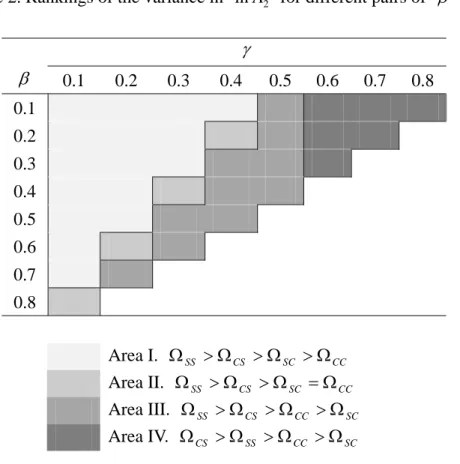
(16) while both of them are at an intermediate level. Again, both the frequency and sequence of ability mixing across schools matter to the role of the parent's background in the determination of the final output, because in CS (but not in SC) educational investments at period 1 may change the quality of school peers at period 2, which in turn improves a student's educational outcome. A rare empirical study by Galindo-Rueda and Vignoles (2005) examining the impacts of student ability on educational attainments across different secondary school systems in the U.K. agrees with our theoretical prediction; ability has a stronger influence on the outcome in a selective system (CS in our model) than in a comprehensive system (CC). However, empirical evidence on the effects of family background on educational outcomes is rather mixed. While Galindo-Rueda and Vignoles (2005) show the role of parental background increased with the transition from a selective to a comprehensive system in U.K. secondary education, Dustmann (2004) and Meghir and Palme (2005) find selective systems (CS) in secondary education reinforce the impact of family background relative to comprehensive systems (CC) in Germany and Sweden, respectively. Although conflicting empirical evidence demands further investigation, institutional features that are missed in our theoretical model and different empirical measures of the educational outcome may be responsible for such a discrepancy. In addition to the elasticities of the education output with respect to student ability and parental income, we next examine another measure of educational equity: the variance of educational outcome--- V (ln A2 ) more specifically. Proposition 3: (Variance of ln A2 ) Let Ω k be the variance of ln A2 in school system k . Let us suppose that, as often empirically found, Cov(ln A0 , ln yT ) > 0 .. (i) (ii). Ω CS > Ω SC Other rankings of variances among Ω CC , Ω SS , Ω CS and Ω SC are not. uniquely determined. Proof: From Table 1,. Ω CC = V (ln A0 ) + 4( β + γ ) 2 V (ln yT ) + 4( β + γ )Cov (ln A0 , ln yT ) ; Ω SS = (1 + β ) 4 V (ln A0 ) + γ 2 (2 + β ) 2 V (ln yT ) + 2γ (2 + β )(1 + β ) 2 Cov(ln A0 , ln yT ) ;. 14.
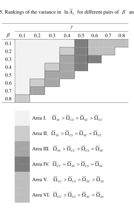
(17) Ω CS = (1 + β ) 2 V (ln A0 ) + [( β + γ )(1 + β ) + γ ] 2 V (ln yT ) + 2(1 + β )[( β + γ )(1 + β ) + γ ]Cov (ln A0 , ln yT );. Ω SC = (1 + β ) 2 V (ln A0 ) + ( β + 2γ ) 2 V (ln yT ) + 2(1 + β )( β + 2γ )Cov(ln A0 , ln yT ) .. Given that Cov(ln A0 , ln yT ) > 0 , propositions (i) and (ii) are trivial. QED Out of a total of six comparisons that can be made for Ω CC , Ω SS , Ω CS and Ω SC , the ranking is uniquely determined only between Ω CS and Ω SC . V (ln A2 ) is larger in CS than in SC. Such a result is primarily driven by the fact that ( β + γ )(1 + β ) + γ > β + 2γ . That is, while the initial difference in child ability contributes to V (ln A2 ) equally in CS and SC, inequality in parental income and the fact that rich parents tend to have smarter children amplify V (ln A2 ) in CS relative to SC. Parental income plays a stronger role in the determination of the educational output in the former than in the latter (proposition 2.(ii)). Similar to the comparisons of other criteria, the sequence as well as the frequency of ability grouping across schools matters to the variance in the final outcome. For the other five comparisons, the rankings fail to be uniquely determined. Since (1 + β ) 4 > (1 + β ) 2 > 1 and 4( β + γ ) 2 > [( β + γ )(1 + β ) + γ ] 2 > ( β + 2γ ) 2 > γ 2 (2 + β ) 2 , the ranking of the component of V (ln A2 ) that is related to each of V (ln A0 ) and V (ln yT ) is determined in the same order that is shown in proposition 2.(i) and 2.(ii). However, the role of Cov(ln A0 , ln yT ) in the determination of V (ln A2 ) is not. uniform across school systems. Therefore, without detail information on the values of β , γ , V (ln A0 ) , V (ln yT ) and Cov(ln A0 , ln yT ) , we do not know a priori which system yields what level of inequality in the final outcome. This finding is in fact in contrast to the conventional belief that the inequality of the educational outcome is larger in selective systems than in comprehensive systems (see Hur and Kang (2007) for the similar finding). In each pair of comprehensive and selective systems the variance of the final outcome depends on a variety of factors such as β , γ , V (ln A0 ) , V (ln yT ) and Cov(ln A0 , ln yT ) . The degree of contribution of each factor to V (ln A2 ) varies according to the school system. Although we do not know definitely which system yields what level of variance in the final outcome, we can at least attempt to draw a rough picture of inequality in different school systems by substituting plausible values for V (ln A0 ) , V (ln yT ) and Cov(ln A0 , ln yT ) . Below we assign values to constituents of V (ln A2 ) that are plausible from previous empirical research. A value of one is assigned to each of. 15.
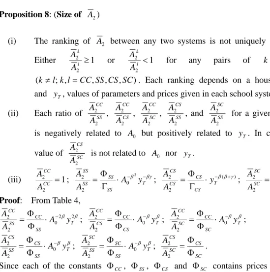
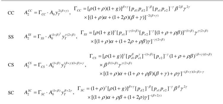
(18) V (ln A0 ) and V (ln yT ) for normalization, and 0.4 to Cov(ln A0 , ln yT ) , since studies on intergenerational income and educational mobility suggest that Cov(ln A0 , ln yT ) is around 0.4 (Solon, 1992; Zimmerman, 1992; Epple and Romano, 1998). Given such values, the rankings of V (ln A2 ) between different school systems are illustrated in Table 2 for varying pairs of β and γ . There are four unique areas in the table. Area I is pairs of β and γ for which V (ln A2 ) is ranked by Ω SS > Ω CS > Ω SC > Ω CC ; area II is those for which Ω SS > Ω CS > Ω SC = Ω CC ; area III is those for which Ω SS > Ω CS > Ω CC > Ω SC ; area IV is those for which Ω CS > Ω SS > Ω CC > Ω SC . Two patterns are noteworthy in Table 2 for the given values of V (ln A0 ) , V (ln yT ) and Cov(ln A0 , ln yT ) . First, for all feasible pairs of β and γ , V (ln A2 ) is larger in the systems that employ the selective method in period 2 (SS and CS) than in those that adopt the comprehensive method in period 2 (CC and SC). This suggests that the comprehensive method in the later stages of schooling is effective in mitigating the inequality of the educational outcome. Second, for a given value of β below 0.4, the ranking of Ω SS and Ω CS reverses as γ rises above 0.5; for a given value of β , the ranking of Ω SC and Ω CC reverses as γ rises. They suggest that as the role of monetary expenditures ( γ ) increases in educational production, the comprehensive method in the early stage of schooling yields a higher variance in the final outcome than the selective method; the variance-reducing function of the comprehensive system weakens as γ rises. Yet the first pattern that the variance is smaller under the comprehensive system at period 2 than under the selective system holds for all feasible pairs of β and γ . Previous research suggests that β is approximately between 0.2 and 0.4 for elementary and secondary school students (Hanushek et al., 2003; Hoxby, 2000; Kang, 2007) and that γ is between 0.1 and 0.2 (Card and Krueger (1996, p.37)). Therefore, for the current given values of V (ln A0 ) , V (ln yT ) and Cov(ln A0 , ln yT ) , the most plausible rankings would be given by Ω SS > Ω CS > Ω SC > Ω CC . Empirical studies are rare that examine the impacts of different school systems on educational inequality. Nonetheless, existing studies such as Gorard and Smith (2004) and Hanushek and Woessmann (2006) conform to our theoretical prediction. They present that a selective system in secondary education (CS in our model) exacerbates the inequality in educational outcomes relative to a comprehensive system (CC in our model). Proposition 4: (Size of A2 ). 16.
(19) (i). The ranking of A2 between any two systems is not uniquely determined. A2k A2k or ≥ 1 < 1 for any pairs of k and l A2l A2l (k ≠ l ; k , l = CC , SS , CS , SC ) . Each ranking depends on a household's A0. Either. and yT , values of parameters and prices given in each school system. (ii). A2CC A2CC A2CC A2CS A2SC , , , , and for a given household is A2SS A2CS A2SC A2SS A2SS negatively related to A0 but positively related to yT . In contrast, the value. Each ratio of. A2CS of SC is not related to A0 but it is positively related to yT . A2 Proof: From Table 1, A2CC ΓCC A2CC ΓCC A2CC ΓCC − β ( 2 + β ) β ( 2 −γ ) − β β (1− β −γ ) = ⋅ A y ; = ⋅ A y ; = ⋅ A0− β yTβ ; 0 0 T T ΓSS A2SS A2CS ΓCS A2SC ΓSC. A2CS ΓCS A2SC ΓSC A2CS ΓCS β ( β +γ ) − β (1+ β ) β (1+ β ) − β (1+ β ) β (1−γ ) = ⋅ A y ; = ⋅ A y ; = ⋅ yT . 0 0 T T A2SS ΓSS A2SS ΓSS A2SC ΓSC Since each of the constants ΓCC , ΓSS , ΓCS and ΓSC contains prices ( p d 1 , p d 2 , p e1 and p e 2 ), its value is indeterminate without further information on the markets in different school systems. Hence comes proposition (i). Proposition (ii) are trivial given the preceding formulas. QED Proposition 4.(i) suggests that it is difficult a priori to decide which sequence of school systems yields greater educational outputs. This is in contrast to previous studies that usually support selective systems as an efficient method of student allocation to schools (e.g., Fernandez and Gali, 1999; Lazear, 2001). These studies in general ignore the possibility that parents may adjust their optimal choices of consumption and educational investments to different grouping methods in school. If parents respond to how to group students across schools, a pool of students to be grouped in a school may be subject to change when different systems of student allocation are adopted in different stages of schooling (e.g., Epple et al, 2002). Our model addresses such a possibility via prices ( p d 1 , p d 2 , p e1 and p e 2 ) at different stages of schooling. Because sorting of students into schools varies by school systems, the ranking of the ultimate educational outcome mediated through peer effects is indeterminate between any two systems. We can only infer that high prices of d and e lead to poor educational outcomes. In line with such theoretical predictions, empirical studies report inconclusive evidence on the impact of school systems on overall educational outcomes. While Kang. 17.
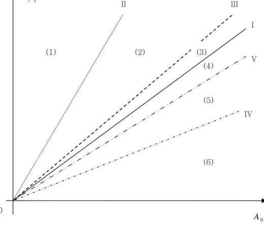
(20) et al. (2007) show that a transition from a selective (CS) to a comprehensive (CC) system in secondary education significantly increased the average educational outcome (i.e., adulthood earnings) in South Korea, Hanushek and Woessmann (2006) find that school systems fail to yield significant differences in the average outcome (i.e., test score in secondary school), using international data sets.11 Proposition 4.(ii) implies that households characterized by different combinations of ( A0 , y1 , y 2 ) prefer different pairs of school systems. Namely, the rankings depend on the values of A0 and yT . In the absence of detail information on the parameter values and prices, however, it is difficult to know a priori which pairs of school systems are liked or disliked by what types of households characterized by ( A0 , yT ). In order to draw a rough picture of the pairs of school systems preferred by different households, as in the case of variance comparisons, we employ a simulation method by substituting plausible values for parameters and prices. The set-up of the simulation is as follows: A value of 0.4 is assigned to β , because peer effects literature suggests values between 0.2 and 0.4 for the effect of average peer quality on a student's achievement (Hanushek et al., 2003; Hoxby, 2000; Kang, 2007); a value of 0.1 is allocated to γ , because Card and Krueger (1996, p.37) summarize that a 10 percent increase in public school spending leads to about a 1-2 percent increase in subsequent earnings; thus α is equal to 0.5; we set all of the prices p d 1 , p d 2 , p e1 and p e 2 equal to one, as we have no useful information on them and wish to avoid arbitrary price differences; finally, we set g = 0.05 and ρ = 0.95 . Figure 1 shows six lines each of which represents the households that are indifferent. 11. Our theoretical model casts doubt on the capability of transnational comparisons to reveal the true. strength of ability grouping (as opposed to ability mixing) in raising the level of educational outputs. Because each country possesses unique educational markets for school districts and private educational services, the prices are likely to differ across countries. Even if parents’ preferences are identical, the educational output may vary across countries solely by the differences in the prices, not by the method of ability grouping in school. Hanushek and Woessmann (2006) attempt to overcome such a problem by applying difference-in-difference methods that use educational outputs of primary and secondary schooling. An implicit assumption of the paper is that there are no substantial differences in markets for school districts and private educational services between primary and secondary education in each country. A before-after comparison for a single country such as Kang et al. (2007) may also be a valid empirical strategy; a similar assumption is that there are no changes in the educational markets in the vicinity of the exogenous policy change.. 18.
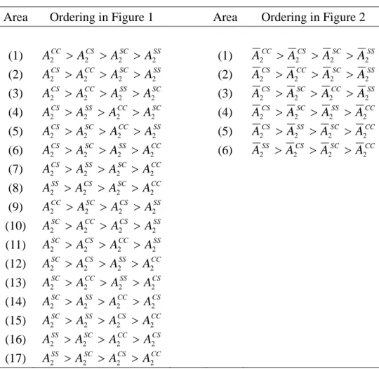
(21) between two school systems in terms of A2 .12 Line I represents the households that are indifferent between CC and SS; Line II those indifferent between CC and CS; Line III those indifferent between CC and SC; Line IV those indifferent between SS and CS; Line V those indifferent between SS and SC; Line VI those indifferent between CS and SC. The six lines divide the entire region by a total of 17 unique areas that are individually numbered from (1) to (17). Table 3 reports the orderings of A2 among four different school systems in a given area. For example, A2CC > A2CS > A2SC > A2SS for households whose ( A0 , yT ) is located in area (1), etc. <Insert Figure 1 and Table 3 here.> From the orderings of A2 in the 17 areas, CC is most preferred by the households in areas (1) and (9), but least preferred by those in areas (6), (7), (8), (12), (15) and (17); SS is most preferred by those in areas (8), (16) and (17), but least preferred by those in areas (1), (2), (5), (9), (10) and (11); CS is most preferred by those in areas (2), (3), (4), (5), (6) and (7), but least preferred by those in areas (13), (14) and (16); SC is most preferred by those in areas (10), (11), (12), (13), (14) and (15), but least preferred by those in areas (3) and (4). Households with low A0 and high yT tend to like CC but dislike SS; households with high A0 and low yT tend to like SS but dislike CC; households with high A0 and high yT tend to like CS but dislike SC; households with low A0 and low yT tend to like SC but dislike CS. In sum, the overall performance of a school system does not only depend on the frequency and sequence of ability grouping across schools. It is also determined by how households are distributed over A0 and yT and how they prefer each school system. Thus which sequence of school systems is adopted in a nation's education system will be ultimately determined by voting of households. Our analysis sheds light on decisions by households and policy-makers by offering comparisons about educational implications that can be produced by four different sequences of school systems. Our analysis also suggests that there always exist conflicts in interests surrounding the choice of school systems, unless policy-makers offer different combinations of school systems in different regions so that households self-select into the most preferred. 12. In addition to comparisons based on A2 , we can employ the total indirect utility (i.e.,. U * = ln U 1* + ρ ln U 2* ) as a criterion of such comparisons. The results based on the utility, however, produce qualitatively similar pictures given here. Such results are available upon request.. 19.
(22) school system. To the extent that policy-makers have to decide over a limited set of school systems in a nation, a nation's school system will ultimately be determined by how they distribute weights to each of educational criteria (e.g., consumption level, the inequality and overall level of the educational outcome, etc) in order to achieve educational goals. The presence of different school systems, as observed in different nations around the globe, will reflect transnational differences in such weights given to each of a variety of educational targets. 4. Educational Implications When the Entrance Exams Signal a Student's Endowed Ability Alone. In the preceding sections we suppose that the entrance exams in selective systems test academic quality of students just prior to the start of school placement. Namely, the entrance exam for period-1 schooling tests the level of A0 , while the exam for period-2 schooling tests the level of A1 . Such exams are, however, one particular type of entrance exams; one can imagine a different setting of entrance exams. For example, an exam can test a student's endowed ability ( A0 ) alone, but not her nurtured ability. An IQ test seems relatively close to such a test, although to what extent an IQ test measures a person's endowed ability remains controversial. Ferdinandez and Gail (1999) and Hur and Kang (2007) suggest that how strongly the entrance exam in the selective system signals a student's endowed ability relative to her nurtured ability matters for educational implications of comprehensive and selective systems. In this section, we extend the ideas of Ferdinandez and Gail (1999) and Hur and Kang (2007) to school systems of different stages of schooling by employing (hypothetical) entrance exams that signal a student's endowed ability alone (but not her nurtured ability) for school admission. We modify the model for θ t by replacing At −1 with A0 , as follows:. θ t = A0τ d tδ t. t. (t = 1, 2). (16). As discussed in section 3, given within-district randomization in comprehensive systems, CC is characterized by τ 1 = τ 2 = 0 and δ 1 = δ 2 = 1 ; SS by τ 1 = τ 2 = 1 and δ 1 = δ 2 = 0 ; CS by τ 1 = 0 , τ 2 = 1 , δ 1 = 1 and δ 2 = 0 ; SC by τ 1 = 1 , τ 2 = 0 , δ 1 = 0 and δ 2 = 1 . Note that the entrance exam of the period-1 selective system remains the same as earlier, and that only the entrance exam of the period-2 selective system has changed. Thus a household's choices under CS and SS alone are expected to be affected, while those under CC and SC remain unaffected.. 20.
(23) A household's new utility function at t is given by: U t = xtα At = xtα { At −1 ( A0τ t d tδ t ) β etγ } = xtα ( A0τ t β At −1 d tδ t β etγ ). (17). The total utility is denoted by: U = α [ln x1 + ρ ln x 2 ] + [(1 + ρ )(1 + βτ 1 ) + ρβτ 2 ] ln A0 + (1 + ρ )[ βδ 1 ln d1 + γ ln e1 ] + ρ[ βδ 2 ln d 2 + γ ln e2 ]. Given the same budget constraint as in section 3, the optimal quantities of choice variables, the educational outcome and indirect utilities are obtained as following: ⎛ α x1* = ⎜⎜ ⎝ (1 + ρ )α + [(1 + ρ )δ 1 + ρδ 2 ]β + (1 + 2 ρ )γ. ⎞ ⎟⎟ ⋅ yT ⎠. (18). ⎛ (1 + ρ ) ⋅ βδ 1 d1* = ⎜⎜ ⎝ (1 + ρ )α + [(1 + ρ )δ 1 + ρδ 2 ]β + (1 + 2 ρ )γ. ⎞ yT ⎟⎟ ⋅ ⎠ pd1. (19). ⎛ (1 + ρ ) ⋅ γ e1* = ⎜⎜ ⎝ (1 + ρ )α + [(1 + ρ )δ 1 + ρδ 2 ]β + (1 + 2 ρ )γ. ⎞ yT ⎟⎟ ⋅ ⎠ p e1. (20). ⎛ ρα x 2* = ⎜⎜ ⎝ (1 + ρ )α + [(1 + ρ )δ 1 + ρδ 2 ]β + (1 + 2 ρ )γ. ⎞ (1 + g ) yT ⎟⎟ ⋅ px2 ⎠. (21). ⎛ ρβδ 2 d 2* = ⎜⎜ ⎝ (1 + ρ )α + [(1 + ρ )δ 1 + ρδ 2 ]β + (1 + 2 ρ )γ. ⎞ (1 + g ) yT ⎟⎟ ⋅ pd 2 ⎠. (22). ⎛ ργ e2* = ⎜⎜ ⎝ (1 + ρ )α + [(1 + ρ )δ 1 + ρδ 2 ]β + (1 + 2 ρ )γ. ⎞ (1 + g ) yT ⎟⎟ ⋅ pe 2 ⎠. (23). At* = A0τ t β At*−1 (d t* ) δ t β (et* ) γ U t* = ( xt* ) α At*. (t = 1, 2). (t = 1, 2). (24) (25). U * = ln U 1* + ρ ln U 2*. (26). 21.
(24) We will also drop the asterisks of the variables. To distinguish from those in section 3, all the optimal values of the variables in this section are over-lined. Table 4 summarizes the consumption levels ( xt ), educational expenditures ( Et ), and the final educational outcome ( A2 ) for each school system. From Table 4 it is easy to show that x1SS > x1SC > x1CS > x1CC and x 2SS > x 2SC > x 2CS > x 2CC , which mirror the rankings in consumption levels in section 3. In both periods 1 and 2 the consumption levels are the largest in SS and the smallest in CC. The levels are larger in SC than those in CS, while both levels are intermediate between SS and CC. It is also noteworthy that while xtCC = xtCC and xtSC = xtSC , xtSS > xtSS and xtCS > xtCS for each t (= 1,2) . If the entrance exam at period 2 tests the level of A0 alone, but not A1 , the consumption levels at both periods rises in SS and CS, which employ the selective method at period 2, while they do not change in CC and SC, which employ the comprehensive method at period 2. Since over-investment for A1 in period 1 does not lead to the change in school peer quality in period 2 even under SS and CS, parents spend less on education and consume more in the new institutional setting than in the old setting where the entrance exam tests the level of A1 . This can be also seen in patterns of educational expenditures that follow. Proposition 5: (Educational Expenditures) (i) E1CS > E1SS > E1CC > E1SC . E 2SC > E 2CC > E 2SS > E 2CS . (ii) ETCC > ETCS > ETSC > ETSS . (iii) E1CC = E1CC ; E1SC = E1SC ; E1SS < E1SS ; E1CS < E1CS (iv) E 2CC = E 2CC ; E 2SC = E 2SC ; E 2SS > E 2SS ; E 2CS > E 2CS (v). (vi). ETCC = ETCC ; ETSC = ETSC ; ETSS < ETSS ; ETCS < ETCS. Proof: (i) Comparisons between two different E1k 's are given as following: E1CC − E1SS = − β [ ρα + (1 + 2 ρ ) β ] × const. < 0 ; E1CC − E1CS = − ρβ × const. < 0 ; E1CC − E1SC = β (1 + ρ ) × const. > 0 ; E1SS − E1CS = − β [(1 + ρ )α + ργ ] × const. < 0 ; E1SS − E1SC = ρβ × const. > 0 ; E1CS − E1SC = β [(1 + ρ )α + ρβ + 2 ργ ] × const. > 0 .. Proposition (i) is trivial. (ii) Comparisons between two different E 2k 's are given as following:. 22.
(25) E 2CC − E 2SS = (1 + ρ )αβ × const. > 0 ; E 2CC − E 2CS = (1 + ρ ) β × const. > 0 ; E 2CC − E 2SC = −(1 + ρ ) β × const. < 0 ; E 2SS − E 2CS = ρβ × const. > 0 ; E 2SS − E 2SC = −(1 + ρ )(α + γ ) β × const. < 0 ; E 2CS − E 2SC = − β [(1 + ρ )(α + β ) + (1 + 3ρ )γ ] × const. < 0 . Proposition (ii) is trivial. (iii) Comparisons between two different ETk 's are given as following: ETCC − ETSS = (1 + ρ )α × const. > 0 ; ETCC − ETCS = ρ (1 + ρ )αβ × const. > 0 ; ETCC − ETSC = (1 + ρ ) 2 αβ × const. > 0 ; ETSS − ETCS = −(1 + ρ ) 2 αβ × const. < 0 ; ETSS − ETSC = − ρ (1 + ρ )αβ × const. < 0 ; ETCS − ETSC = (1 + ρ )αβ × const. > 0 . Proposition (iii) is trivial. (iv) Comparisons between E1k and E1k are given as following: From Tables 1 and 4, it is obvious that E1CC = E1CC and E1SC = E1SC . E1SS − E1SS = ρβγ [(1 + ρ )α + ργ ] × const. > 0 ; E1CS − E1CS = ρβ ( β + γ )[(1 + ρ )α + ργ ] × const. > 0 . (v) Comparisons between E 2k and E 2k are given as following: It is obvious that E 2CC = E 2CC and E 2SC = E 2SC . E 2SS − E 2SS = − ρβγ × const. < 0 ; E 2CS − E 2CS = − ρβ ( β + γ ) × const. < 0 . (vi) Comparisons between ETk and ETk are given as following: It is obvious that ETCC = ETCC and ETSC = ETSC . ETSS − ETSS = ρ (1 + ρ )αβ × const. > 0 ; ETCS − ETCS = ρ (1 + ρ )αβ ( β + γ ) × const. > 0 . QED If the entrance exam in the period-2 selective system tests A0 alone, patterns of educational spending across school systems remain similar to those in proposition 1. A household's educational expenditure at period 1 is the largest in CS and the smallest in SC. In contrast to proposition 1.(i), the expenditure at period 1 is always lower in CS than in SC. The educational expenditure at period 2 is the largest in SC and the smallest in CS; the period-2 expenditure in CC are greater than that in SS, while both being at an intermediate level. The total expenditure is the largest in CC and the smallest in SS; in the middle, it is larger in CS than in SC. Propositions 5.(iv) to 5.(vi) suggest that once the entrance exam in the period-2 selective system tests A0 alone, the sizes of educational expenditure in SS and SC changes relative to those in the old exam setting, but the direction varies by the period. While the expenditures in CC and SC remain constant in both periods, the educational expenditures in SS and CS fall in period 1 but rise in period 2; overall, the total educational expenditures in SS and CS alike fall if the A0 -biased entrance exam is. 23.
(26) offered at period 2. Such changes take place primarily because over-investment for A1 at period 1 does not lead to the improvement in school peer quality at period 2 in SS and CS under the new exam setting; parents would rather choose to consume more in the new institutional setting. Such patterns in educational spending and consumption in turn give rise to differences in the role of family income (and student endowed ability) in determining the final educational outcome ( A2 ) under the new exam setting. Proposition 6: (Elasticities of A2 ). (i). η ASS0 > η ACS0 = η ASC0 > η ACC 0. (ii). η yCC > η yCS = η ySC > η ySS. (iii). CC SS SS CS CS SC SC η ACC 0 = η A0 ; η A0 < η A0 ; η A0 = η A0 ; η A0 = η A0 .. (iv). η yCC = η yCC ; η ySS < η ySS ; η yCS < η yCS ; η ySC = η ySC .. Proof: SS From Table 4, η ACC and η ACS0 = η ASC0 = 1 + β . η yCC = 2( β + γ ) , 0 = 1 , η A0 = 1 + 2 β. η ySS = 2γ and η yCS = η ySC = β + 2γ . Propositions (i) and (ii) are trivial. Comparisons with Table 1 show propositions (iii) and (iv). QED As in proposition 2, the child-ability elasticity η A0 is the largest in SS and the smallest in CC, while it is at an intermediate level in CS and SC; the family-income elasticity η y is the largest in CC and the smallest in SS, while it is at an intermediate level in CS and SC. A difference from proposition 2.(ii) is that η y is equal between CS and SC, since educational spending at period 1 does not lead to the change in school peer quality at period 2. Proposition 6.(iii) suggests that since peer quality in period-2 schooling is less affected by the initial difference in A0 under the new setting, η A0 falls in SS, while it remains constant in CC, CS and SC. Proposition 6.(iv) suggests that η y falls in SS and CS under the new setting of the entrance exam, because over-investment for A1 fail to. 24.
(27) change the peer quality in period-2 schooling. Such patterns in elastisticies are reflected in the variance in ln A2 for each school system. Proposition 7: (Variance of ln A2 ) Let us suppose that Cov(ln A0 , ln yT ) > 0 .. (i). Ω CS = Ω SC. (ii). Other rankings of variances among Ω CC , Ω SS , Ω CS and Ω SC are not uniquely determined.. (iii). Ω CC = Ω CC ; Ω SS < Ω SS ; Ω CS < Ω CS ; Ω SC = Ω SC .. Proof: From Table 4,. Ω CC = V (ln A0 ) + 4( β + γ ) 2 V (ln yT ) + 4( β + γ )Cov (ln A0 , ln yT ) ; Ω SS = (1 + 2β ) 2 V (ln A0 ) + 4γ 2V (ln yT ) + 4γ (1 + 2β )Cov(ln A0 , ln yT ) ; Ω CS = Ω SC = (1 + β ) 2 V (ln A0 ) + ( β + 2γ ) 2 V (ln yT ) + 2(1 + β )( β + 2γ )Cov(ln A0 , ln yT ) .. Given that Cov(ln A0 , ln yT ) > 0 , propositions (i) and (ii) are trivial. From comparisons with Table 4, it is obvious that Ω CC = Ω CC and Ω SC = Ω SC ; Ω SS − Ω SS = β 2 (2 + 4 β + β 2 )V (ln A0 ) + β (4 + β )V (ln yT ) + β (1 + 4 β + β 2 )Cov (ln A0 , ln yT ) > 0;. Ω CS − Ω CS = ( β + γ ){β [2( β + 2γ ) + β ( β + γ )]V (ln yT ) + 2β (1 + β )Cov(ln A0 , ln yT )} > 0. . QED As in proposition 3, the ranking is uniquely determined only between Ω CS and Ω SC . V (ln A2 ) is equal between CS and SC. Since the entrance exams tests A0 alone. in both periods 1 and 2, educational spending at period 1 does not lead to the change in school peer quality at period 2; the initial difference in A0 also change school peer quality equally in CS and SC. Other rankings fail to be uniquely determined, because. 25.
(28) the variance depends on many factors that countervail across different school systems. Although the ranking of the component of V (ln A2 ) that is related to each of V (ln A0 ) and V (ln yT ) is determined as in propositions 6.(i) and 6.(ii), respectively, the role of Cov(ln A0 , ln yT ) in the determination of V (ln A2 ) is not uniform across school systems. Proposition 7.(iii) suggests that while it remains constant in CC and SC, V (ln A2 ) falls in SS and CS under the new setting of the entrance exam. Again, it is primarily because peer quality in period-2 schooling is less affected by the initial difference in A0 under the new setting, and over-investment for A1 fails to increase the peer quality in period-2 schooling. Since we do not know a priori which system yields what level of inequality in the final outcome, we attempt to draw a rough picture of V (ln A2 ) in different school systems by substituting V (ln A0 ) for one, V (ln yT ) for one and Cov(ln A0 , ln yT ) for 0.4, as in section 3. Given such values, the rankings of V (ln A2 ) are illustrated in Table 5 for varying pairs of β and γ . There are six unique areas in the table. A notable pattern is that for a given value of β below 0.3, the ranking of Ω SS and Ω CC dramatically reverses as γ rises above 0.5. For β below 0.3, Ω SS is the largest and Ω CC is the smallest if γ is below 0.5. In stark contrast, Ω SS is the smallest and Ω CC is the largest if γ is above 0.5. This suggests that, if the role of peer quality ( β ) is relatively weak in educational production but that of educational expenditure ( γ ) is relatively strong, comprehensive systems amplify initial inequality of family income but selective systems narrow it in the determination of the final educational output. In such a case, selective systems are more effective to reduce inequality in educational attainments to the extent that the entrance exams test A0 alone in selective systems. See Hur and Kang (2007) for the similar finding. Previous research, however, suggests that β is approximately between 0.2 and 0.4 and that γ is between 0.1 and 0.2. Therefore, for the current given values of V (ln A0 ) , V (ln yT ) and Cov(ln A0 , ln yT ) , the most plausible rankings would be given by Ω SS > Ω CS = Ω SC > Ω CC .. 26.
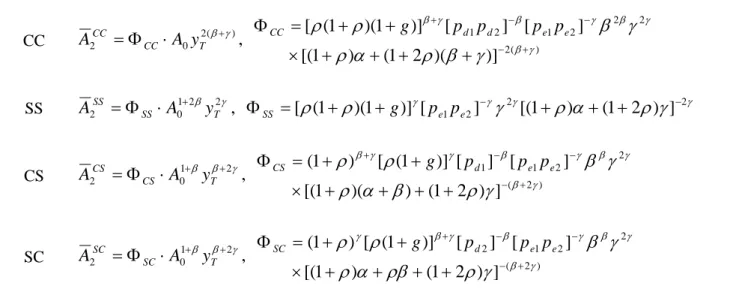
(29) Proposition 8: (Size of A2 ). (i). The ranking of A2 between any two systems is not uniquely determined. A2k A2k ≥ 1 or < 1 for any pairs of k and l Either A2l A2l (k ≠ l ; k , l = CC , SS , CS , SC ) . Each ranking depends on a household's A0 and yT , values of parameters and prices given in each school system.. (ii). A2CC A2CC A2CC A2CS A2SC Each ratio of , , , , and for a given household A2SS A2CS A2SC A2SS A2SS is negatively related to A0 but positively related to yT . In contrast, the value of. (iii). A2CS is not related to A0 nor yT . A2SC. A2CC A2SS Φ SS A2CS Φ CS − β ( β +γ ) A2SC − β 2 − βγ ; = 1 = ⋅ A y ; = ⋅ yT ; = 1. 0 T ΓSS ΓCS A2CC A2SC A2SS A2CS. Proof: From Table 4, A2CC Φ CC A2CC Φ CC A2CC Φ CC −2 β 2 β −β β = ⋅ A0 yT ; = ⋅ A0 yT ; = ⋅ A0− β yTβ ; SS CS SC Φ SS Φ CS Φ SC A2 A2 A2. A2CS Φ CS A2CS Φ CS A2SC Φ SC −β β −β β = ⋅ A0 yT ; = ⋅ A0 yT ; . = A2SC Φ SC A2SS Φ SS A2SS Φ SS Since each of the constants Φ CC , Φ SS , Φ CS and Φ SC contains prices ( p d 1 , p d 2 , p e1 and p e 2 ), its value is indeterminate without further information on the markets in different school systems. Hence comes proposition (i). Proposition (ii) are trivial given the preceding formulas. Proposition (iii) is obvious from comparisons between Tables 1 and 4. QED Proposition 8.(i) suggests that it is difficult a priori to decide which sequence of school systems yields greater educational outputs, as in proposition 4.(i). However, proposition 8.(ii) implies that households characterized by different combinations of ( A0 , y1 , y 2 ) prefer different pairs of school systems. The rankings depend on the values of A0 and yT . Here we also employ a simulation method by substituting the same values for parameters and prices as in section 4. Figure 2 shows five lines each of which represents the households that are indifferent between two school systems in terms of A2 . (For the current given values, CS is preferred to SC by every household.) Each line represents the households that are indifferent between the same pairs of the school systems as in Figure 1. The five lines. 27.
(30) divide the entire region by a total of 6 unique areas. Table 3 (right panel) reports the orderings of A2 among four school systems in a given area. From the orderings of A2 , CC is most preferred by the households in area (1), but least preferred by those in areas (4), (5) and (6); SS is most preferred by those in area (6), but least preferred by those in areas (1), (2) and (3); CS is most preferred by those in areas (2), (3), (4) and (5). Namely, households with low A0 and high yT tend to like CC but dislike SS; households with high A0 and low yT tend to like SS but dislike CC; households with medium A0 and medium yT tend to like CS but dislike SS or CC, depending on their characteristics. The conclusion is similar to that in section 3. In the new setting of the entrance exam also, the overall performance of a school system does not only depend on the frequency and sequence of ability grouping across schools, but on how households are distributed over A0 and yT and how they prefer each school system. Proposition 8.(iii) suggests that the rankings between A2SS and A2SS , on the one hand, and between A2CS and A2CS , on the other, also vary by household characteristics, while the final outcomes are equal between the old and new settings in CC and SC. A2SS is greater (smaller) than A2SS for households with small (large) values of both A0 and yT . In contrast, A2CS is greater (smaller) than A2CS for households with small (large) yT , while A0 does not affect the preference ranking. Thus whether or not the entrance exam should be biased toward A0 in the selective system will be ultimately determined by voting of households, given the fact that each type of the exam chosen has the educational implications that are outlined in our preceding discussions. This reveals the conflicts in interests surrounding the choice of school systems and exam settings as shown in section 3. Similarly, the ultimate decision will be made based on a society's weights given to a variety of educational targets. 5. Concluding Remarks. In this paper, using a simple two-period model of household choices, we consider four different school systems of student allocation at different stages of schooling and their educational implications. Our model first suggests that both the frequency and sequence of ability grouping play an important role in producing educational implications of school systems. We next find that different households that are characterized by a pair of family income and the child's innate ability prefer different combinations of school systems. As a result, the overall performance of a school system. 28.
(31) is determined by how households are distributed over income and a child's ability. Which sequence of school systems is adopted in a nation's education system will be ultimately determined by voting of households. Finally, if the entrance exam in the selective system tests a student's endowed ability alone but never her nurtured ability, then the systems that adopt the selective method in the later stage of education show more favorable educational implications than if the exam tests a student's endowed ability as well as her nurtured ability. Whether or not the entrance exam should signal the endowed ability alone in the selective system will also be determined by voting of households, because different households prefer different settings of the entrance exam in the selective system. Although useful policy implications can be drawn from our approach, it is not, of course, free of drawbacks. First, the model is based on partial equilibrium, where prices are fixed across different school systems. In the context of general equilibrium, however, the prices vary by the structure of markets. We do not model the changes in markets in response to those in demand for each in different school systems. Second, our education production is based on a Cobb-Douglas form, where peer-effects increase with a student's ability (i.e., A = bθ β e γ ). Such a form of peer effects are frequently used in economic theories of education (e.g., Fernandez and Gali, 1999; Lazear, 2001). By assuming a Cobb-Douglas form, we avoid complications that may be introduced by different functional forms of educational production. Nevertheless, there is a need to employ different specifications of peer effects over ability in educational production for future research.. 29.
Figure
+7
Related documents
