On Smooth Density Estimation for Circular Data1 Yogendra P. Chaubey
Department of Mathematics and Statistics, Concordia University, Montr´eal, QC H3G 1M8
e-mail: [email protected]
Abstract
Fisher (1989: J. Structural Geology11, 775-778) outlined an adaptation of the linear kernel estima-tor for density estimation that is commonly used in applications. However, better alternatives are now available based on circular kernels; see e.g. Di Marzio, Panzera, and Taylor, 2009: Statistics & Probability Letters 79, 2066-2075. This paper provides a short review on modern smoothing methods for density and distribution functions dealing with the circular data. We highlight the usefulness of circular kernels for smooth density estimation in this context and contrast it with smooth density estimation based on orthogonal series. It is seen that the wrapped Cauchy kernel as a choice of circular kernel appears as a natural candidate as it has a close connection to orthogonal series density estimation on a unit circle. In the literature the use of von Mises circular kernel is investigated (see Taylor, 2008: Computational Statistics & Data Analysis 52, 3493-3500), that requires numerical computation of Bessel function. On the other hand, the wrapped Cauchy kernel is much simpler to use. This adds further weight to the considerable role of the wrapped Cauchy distribution in circular statistics.
Keywords: circular kernels; kernel density estimator; orthogonal polynomials; orthogonal series density
1. Introduction
Given an i.i.d. d−variate random sample {X1, ..., Xn} from a continuous distribution function F
with density f, the Parzen-Rosenblatt kernel density estimator is given by ˜ f(x;h)≡n−1h−d n X i=1 K x−Xi h (1.1) where h is known as the window-width or band-width and K is called the kernel function. The band-width h typically tends to 0 as the sample size n tends to infinity and K is typically a sym-metric density function centered around zero with unit variance. This estimator was proposed by Rosenblatt’s (1956), that was further studied by Parzen (1962) and popularized in many subsequent papers. An alternative motivation for the kernel density estimator is provided recently in Chaubey et al. (2012) by smoothing the empirical distribution function that justifies the use of asymmetric kernels while considering density estimation for non-negative random variables.
1Expanded version of the Invited Paper for the invited session IPS-114, “Nonparametric Methods : Theory and Applications” at ISI-2017, Marrakech July 16-21, 2017
In what follows we consider estimation of the density for circular data, i.e. an absolutely continuous (with respect to the Lebesgue measure) circular density f(θ), θ∈[−π, π],i.ef(θ) is 2π−periodic,
f(θ)≥0 for θ∈R and
Z π
−π
f(θ)dθ= 1. (1.2)
Given a random sample{θ1, ...θn}for the above density, the kernel density estimator may be written
as ˜ f(θ;h) = 1 nh n X i=1 K θ−θi h . (1.3)
Fisher (1989) proposed non-parametric density estimation for circular data by adapting the linear kernel density estimator (1.1) with a quartic kernel [see also Fisher (1993), §2.2 (iv) where an improvement is suggested], defined on [−1,1],that is given by
K(θ) =
(
.9375(1−θ2)2 for −1≤θ≤1;
0 otherwise. (1.4)
[see Eqs. (4.40) and (4.41) of Fisher (1993).] Since the resulting estimator is not necessarily periodic, Fisher (1993) suggested to perform the smoothing by replicating the data to 3 to 4 cycles and considering the part in the interval [−π, π].This problem is easily circumvented by using circular kernels, that has been investigated by Di Marzio et al. (2011). Taylor (2008) considered the von Misses circular normal distribution with concentration parameter κ forK,that gives the estimator forf as ˆ fvM(θ;κ) = 1 n n X i=1 KvM(θ;θj, κ), (1.5) where KvM(θ;µ, κ) = 1
2πI0(κ)exp{κcos(θ−µ)}, −π ≤θ≤π, (1.6) and discussed determination of the optimal data based choice for κ. Note that the von Mises dis-tribution gets concentrated around µfor largeκ.
In Section 2, I present a simple approximation theory motivation for considering the circular kernel density estimator given in (1.5). It may be noted that the wrapped Cauchy distribution with location parameter µand concentration parameter ρis given by
KW C(θ;µ, ρ) =
1 2π
1−ρ2
1 +ρ2−2ρcos(θ−µ) ,−π ≤θ < π, (1.7) that becomes degenerate at θ = µ as ρ → 1. The estimator of f(θ) based on the above kernel is given by ˆ fW C(θ;ρ) = 1 n n X i=1 KW C(θ;θj, ρ). (1.8)
Section 3 describes the approach of approximation using orthogonal functions in deriving density estimators and Fourier series density estimator is highlighted as a special case. This section also establishes the equivalence between the circular kernel estimator using wrapped Cauchy kernel and orthogonal series estimation of a specific complex function defined over a unit circle. In Section 4,
some alternative approaches based on transformations are provided. The last section provides some examples and conclusions.
2. Motivation for the Circular Kernel Density Estimator
We consider the following theorem from approximation theory (see Mhaskar and Pai (2000)) to motivate the circular kernel density estimator. Before giving the theorem we will need the following definition:
Definition 2.1 Let {Kn} ⊂ C∗ where C∗ denotes the set of periodic analytic functions with a
period 2π. We say that {Kn} is an approximate identity if
A. Kn(θ)≥0 ∀ θ∈[−π, π];
B. Rπ
−πKn(θ) = 1;
C. limn→∞max|θ|≥δKn(θ) = 0 for every δ >0.
The definition above is motivated from the following theorem which is similar to the one used in the theory of linear kernel estimation (see Prakasa Rao (1983)). Also, note that we have replaced Kn of Mhaskar and Pai (2000)) by 2πKn without changing the result of the theorem.
Theorem 2.1 Let f ∈C∗,{Kn} be approximate identity and forn= 1,2, ... set
f∗(θ) = Z π −π f(η)Kn(η−θ)dη. (2.9) Then we have lim n→∞θ∈sup[−π,π]|f ∗(θ)−f(θ)|= 0. (2.10)
Note that taking the sequence of concentration coefficients ρ ≡ ρn such that ρn → 1, the density
function of the Wrapped Cauchy will satisfy the conditions in the definition in place of Kn. In
generalKn,appearing in the above theorem may be replaced by a sequence of periodic densities on
[−π, π],that converge to a degenerate distribution atθ= 0.
For a given random sample of θ1, ..., θn from the circular densityf, the Monte-Carlo estimate off∗
is given by ˜ f(θ) = 1 n n X i=1 Kn(θi−θ). (2.11)
The kernel given by the wrapped Cauchy density satisfies the assumptions in the above theorem that provides the estimator proposed in (1.8). This gives the motivation for considering circular kernels for nonparametric density estimation for circular data as proposed in discussed in a more detailed by Marzio MD, et al. (2009). However, their development considers circular kernels of order r = 2 that further requires
Z π
−π
sinj(θ)Kn(θ)dθ= 0 for 0< j <2.
The circular kernel density estimator based on the wrapped Cauchy weights is given by ˜ fW C(θ) = 1 n n X i=1 fW C(θi−θ). (2.12)
that may be considered more convenient in contrast to the von Mises kernel due to the fact that it does not require computation of an integral I0(κ). Another justification of the circular kernel density estimator may presented by smoothing the empirical distribution function, an approach investigated in Babu, Canty and Chaubey (2002) and Babu and Chaubey (2006)[see also the recent paper by Chaubey et al. (2012)].
In this approach we approximate the distribution function instead of the density function using the approximation F∗(θ) = Z π −π F(η)Kn(η−θ)dη = 1− Z π −π Ψθ,n(η)dF(η) (2.13)
where Ψθ,n(.) is the sequence of distribution functions corresponding to the circular densitiesKn(.−
θ)
Since F is unknown, using the edf as a plug-in estimate to estimate F∗, results into an smooth estimator of F given by ˜ F(θ) = 1− Z 2π 0 Ψθ,n(η)dFn(η) = 1− 1 n n X i=1 Ψθ,n(θi). (2.14)
Considering circular distributions with meanµand concentration parameter ρn→0 asn→ ∞,let
the density function corresponding to Ψθ,ncorrespond to a location family given byψ(θ−µ;ρ) that
has meanµand concentration parameterρ,then a smooth density estimator ˜f(θ) (as the derivative of ˜F(θ) is given by ˜ f(θ) = 1 n n X i=1 ψ(θi−θ;ρ). (2.15)
which is of the same form as the circular kernel density estimator given in (2.11).
In the next section we provide details of the approach where the circular density is represented as a linear form using a set of basis functions.
3. Density Estimators using Approximation by Orthogonal Functions
Here we will consider approximating continuous bounded functions f(x) in a compact interval
I = [a, b]⊂R. For a given nonnegative functionw(x) defined on I,the L2 weighted norm of f(x) is defined as
kfkw2 =
Z b
a
|f(x)|2 w(x)dx. (3.16) The space of such functions will be denoted byLw2.The general method of approximation of functions f ∈Lw
2 involves the set of basis functions{ϕk(x)}∞0 and a non-negative weight function w(x) such that < ϕk, ϕk0 >w= Z b a ϕk(x)ϕk0(x)w(x)dx= ( 0 fork6=k0 1 fork=k0 (3.17)
Then for f ∈Lw
2 the partial sum
fN(x) = N X k=0 gkϕk(x), (3.18) where gk= Z b a f(x)ϕk(x)w(x)dx, (3.19)
is considered to be the ‘best’ approximation in terms of the fact that the coefficients gk are such
that ak =gk minimise
kf −fNkw2 =
Z b
a
|f(x)|2 w(x)dx. (3.20) The original idea is attributed to ˇCencov (1962) that considered the cosine basis
{ϕ0(x) = 1, ϕj(x) =
√
2 cos(πjx), j= 1,2, ...}
andw(x) = 1.In recent literature, many other type of basis functions including trigonometric, poly-nomial, spline, wavelet and others have been considered. The reader may refer to Devroy and Gy¨orfi (1985), Efromvich (1999), Hart (1997), Walter (1994) for a discussion of different bases and their properties. Efromvich (2010) presents an extensive overview of density estimation by orthogonal series concentrated on the interval [0,1].As mentioned in Efromvich (2010) the choice of the basis function primarily depends on the support of the function. Thus for the densities on (−∞,∞),or on [0,∞), Hermite and Laguerre series are recommended; see Devroye and Gy¨orfy (2001), Walter (1994), Hall (1980) and Walter (1977). For compact intervals,trigonometric (or Fourier)series are recommended; discussion about these can be found in ˇCencov (1980), Devroy and Gy¨orfy (1985), Efromvich (1999), Hart (1997), Silverman (1986), Hall (1981), Tarter and Lock (1993). Classical orthogonal polynomials such as Chebyshev, Jacobi, Legendre and Gegenbauer are also popular; see Trefthen (2013)), Rudzkis and Radavicius (2005) and Buckland (1992). Wavelet bases are be-coming increasingly popular, due to their ability in visualizing local frequency fluctuations and discontinuities, even though their explicit form is not available.
Once the basis functions are chosen, the density f(x) for a random sample {x1, ..., xn} may be
estimated by ˆ fN(x) = N X k=0 ˆ gkϕk(x), (3.21) where ˆ gk= 1 n n X i=1 ϕk(xi). (3.22)
Efromvich (2010) discusses in detail various strategies of selectingN,albeitin a more general setting by considering the density estimators of the form
ˆ f(x) = ˆf(x,{wˆk}) = ∞ X k=0 ˆ wkgˆkϕk(x) (3.23)
that includes the truncated estimator ˆfJ as well ashard-thresholdingand block-thresholding
estima-tors, commonly studied in the wavelet literature. However, this modification will not be pursued in further discussion.
The estimators using orthogonal series of cosine functions and Fourier series are easy to implement. Using the truncated cosine series, the density estimator is given by
ˆ fOC(θ) = 1 2π + N X k=1 ˆ gkcos(kθ). (3.24) where ˆ gk = 1 nπ n X i=1 cos(kθi).
This is appropriate for circular density functions that are symmetric around zero, however, the Fourier series is more general. The truncated Fourier series off(θ) is given by
f(θ)≈ 1 2a0+ N X k=1 {akcos(kθ) +bksin(kθ)}, (3.25) where ak = 1 π Z π −π f(θ) cos(kθ)dθ, k= 0,1, ..., N (3.26) bk = 1 π Z π −π f(θ) sin(kθ)dθ, k= 1, ..., N. (3.27) Considering these coefficients as expectations of appropriate functions, they can be estimated as
ˆ ak = 1 nπ n X i=1 cos(kθi);k= 0,1,2.... (3.28) ˆbk = 1 nπ n X i=1 sin(kθi);k= 1,2.... (3.29)
Thus, the Fourier series density estimator is given by ˆ fF S(θ) = 1 2π + N X 1 {ˆakcos(kθ) + ˆbksin(kθ)}. (3.30)
N is considered a smoothing parameter and may be determined using the cross-validation method described in Efromvich (2010). A common problem with truncation in these estimators is that it may not produce a true density. In order to alleviate this problem Efromvich (1999) considers L2 projection of ˆf onto a class of non-negative densities given by
˘
f(x) = max(0,fˆ(x)−c), (3.31) where cis chosen to make ˘f a proper density.
Recently, Chaubey (2016) demonstrated an interesting connection between the circular kernel den-sity estimator using the Cauchy kernel and orthogonal series on a circle for the function
W(z) = Z eiτ+z eiτ−z f(τ)dτ. (3.32)
This involves the real and complex Poisson kernels that are defined as Pr(θ, ϕ) =
1−r2
1 +r2−2rcos(θ−ϕ) (3.33)
forθ, ϕ∈[−π, π) andr ∈[0,1) and by
C(z, ω) = ω+z
ω−z (3.34)
for ω ∈ ∂D and z ∈ D;D = {z | |z| < 1}, is the open unit disk and ∂D = {z | |z| = 1} is the boundary of the unit disk. The connection between these kernels is given by the fact that
Pr(θ, ϕ) = Re C(reiθ,eiϕ) = (2π)fW C(θ;ϕ, ρ). (3.35)
where z = reiθ for r ∈ [0,1), θ ∈ [−π, π] and i = √−1. Using the result (see (ii) in §5 of Simon (2005)) that for Lebesgue a.e. θ,
f(θ) = 1
2π limr↑1Re W(re
iθ), (3.36)
a smooth density estimator is proposed to be ˆ fr(θ) =
1
2πReWn(re
iθ) (3.37)
by appropriately choosing r, where
Wn(z) = 1 n n X j=1 eiθj +z eiθj −z . (3.38)
Thus the sample estimate of ˆfr(θ) can be written as
ˆ fr(θ) = 1 n n X j=1 fW C(θ;θj, r). (3.39)
On the other hand the Fourier expansion of W(z) with respect to the basis{1, z, z2, ...} is given by W(z) = 1 + 2 ∞ X j=1 cjzj (3.40) where cj = Z e−ijθf(θ)dθ,
is the jth trigonometric moment. The series is truncated at some term N∗ so that the the error is negligible. However, we show below that estimating the trigonometric moments cj, j= 1,2, ... as
ˆ cj = 1 n n X k=1 e−ijθk,
the estimator of W(z) given by ˆW(z) = 1 + 2P∞j=1cˆjzj is the same as Wn(z).We have ˆ W(z) = 1 + 2 n n X j=1 { ∞ X k=1 e−ikθjzk} = 1 + 2 n n X j=1 { ∞ X k=1 (¯ωjz)k};ωj = eiθj; ¯ωj = e−iθj = 1 + 2 n n X j=1 ¯ ωjz 1−ω¯jz = 2 n n X j=1 1 2 + ¯ ωjz 1−ω¯jz = 1 n n X j=1 1 + ¯ωjz 1−ω¯jz = 1 n n X j=1 C(z, ωj),
which is the same as Wn(z) given in (3.38). This ensures that the orthogonal series estimator of
the density coincides with the circular kernel estimator, using the wrapped Cauchy kernel. 4. Transformation Based Density Estimators
In this section we outline some simple transformation estimators that are based on the fact that if we transform the angular data on (−π, π) to some intervalI,where the properties of approximations on I are well known. Let x=t(θ) denote a one-to-one 2π periodic transformation from (−π, π) to I and let p(x) denote the density of the transformed data, then the density of the original data is given by
f(θ) =p(t(θ))|dt(θ)
dθ |. (4.41)
4.1. Transformation for use with the kernel estimator on the real line
Denoting the angular random variable by Θ, the kernel density estimator on the real line may be applied using the transformation
X= tan(Θ/2), (4.42)
that transforms the interval [pi, π] to (−∞,∞) and the kernel density estimator ofX is given by ˆ p(x;h) = 1 nh n X i=1 K x−tan(θi/2) h . (4.43)
and the transformation based kernel density estimator of f(θ) is given by ˆ f(θ;h) = 1 1 + cos(θ) pˆ sinθ 1 + cosθ;h . (4.44)
An attractive feature of the above procedure in contrast to Fisher’s adaptation of the linear method is that the latter method gives a periodic estimator, however the former does not.
4.2. Transformation for use with Bernstein polynomial density estimator
Babu and Chaubey (2006) consider estimating the distributions defined on a hypercube, extending the univariate Bernstein polynomials (Babu, Canty and Chaubey (2002), Vitale (1973)). Denoting the empirical distribution function of a random sample of n−observations from a random variable X ∈[0,1],by Gn,the Bernstein polynomial density estimator is given by
ˆ pB(x;m) =m m X j=1 Fn j m −Fn j−1 m β(x;j, m−j+ 1), x∈[0,1], (4.45) where β(x;a, b) is given by β(x;a, b) = 1 B(a, b)x a−1(1−x)b−1, (4.46) and B(a, b) = (a+b−1)!/[(a−1)!(b−1)!].We consider the transformation
t(θ) = 1 2+
1 πtan
−1(ctan(θ/2)), (4.47)
that maps the interval [−π, π] to [0,1] in a one-to-one monotonic transformation for all c > 0. Note that this provides a periodic transformation in contrast to the linear transformation t(θ) = θ/(2π) for transforming the interval [0,2π] to [0,1], as considered Carnicero et al. (2010). This transformation offers an extra parametercthat may be optimally chosen for a given random sample. The transformed estimator of f(θ) is given by
ˆ fB(θ;m) = 1 2πpˆB(t(θ);m) c(1 +tan2(θ/2) 1 +c2tan2(θ/2). (4.48)
4.3. Transformation for use with orthogonal polynomials
Orthogonal polynomials of the Chebyshev’s class on [−1,1] can be converted to orthogonal polyno-mials on a circle C={z|kzk= 1}through the transformation
x= 1 2(z+z
−1).
This has been quite popular in numerical approximation of functions (see for example Trefethen (2013), Chapter 3). the kth Chebyshev polynomial can be defined by the real part of the function zk on the unit circle:
x= 1 2(z+z −1) = cosθ, θ= cos−1x, (4.49) Tk(x) = 1 2(z k+z−k) = cos(kθ). (4.50)
The following theorems justify the use of orthogonal polynomial estimators (see Rudin (1976)). Theorem 4.2 If h is Lipschitz continuous on [−1,1],it has a unique representation as Chebyshev series, h(x) =1 2 a0+ ∞ X k=1 akTk(x), (4.51)
which is absolutely and uniformly convergent. The coefficients are given by the formula ak= 2 π Z 1 −1 h(x)Tk(x) √ (1−x2)dx, (4.52)
and for k= 0, by the same formula with the factor2/π changed to 1/π. If h(x) represents a density on [−1,1], ak can be estimated by
ˆ a0 = 1 nπ n X i=1 1 √ (1−x2 i) , (4.53) ˆ ak = 2 nπ n X i=1 Tk(xi) √ (1−x2i);k= 1,2, ... (4.54) (4.55) For using Chebyshev’s polynomials in order to provide circular density estimator we transform the circular data asxi= 2 tan−1(tan(θi/2))/πthat essentially provides a 2π periodic transformation to
the interval [−1,1],and the Chebyshev’s polynomial circular density estimator is given by ˆ fCP(θ) = 1 2πˆa0+ 1 π N X k=1 ˆ akTk(θ/π) (4.56)
The Chebyshev weight function, however, is singular at the extremes of the interval of support. Arbitrary power singularities may be assigned to each extreme giving a general weight function
w(x) = (1−x)α(1 +x)β (4.57) where α, β > 0 are parameters. The associated polynomials are known as Jacobi polynomials, usually denoted as{Pn(α,β}.The special caseα=β,gives orthogonal polynomials that are known as
asGegenauerorultraspherical polynomialsand are subject of much discussion in numerical analysis; see Koornwinder et al. (2010). The most special case of all α = β = 0 gives a constant weight function and produces what are known as Legendre polynomials denoted by Pn(x), n = 0,1,2, ....
that define a orthogonal system for the interval [−1,1].They may be simply described as
P0(x) = 1, P1(x) =x (4.58) and the recurrence relation
(k+ 1)Pk+1(x) = (2k+ 1)xPk(x)−kPk−1(x). (4.59) Thus P2(x) = 3 2x 2−1 2, P3(x) = 5 2x 3−3 2x, ...etc. (4.60)
An explicit representation may be given by the following formula: Pk(x) = 2k k X j=0 k j k+j−1 2 k xj (4.61)
This avoids the possible numerical problem in computing the coefficients due to singularity at the extremes. Hence this will be a preferred alternative to the Chebyshev polynomials. The expansion of a function h(x) in terms of the Legendre polynomials is given by
h(x) = ∞ X k=0 ckPk(x) (4.62) where ck = 1 + 2k 2 Z 1 −1 h(x)Pk(x)dx. (4.63)
Unbiased estimators of the coefficientsck are given by
ˆ ck= 1 + 2k 2n n X i=1 Pk(xi). (4.64)
Thus the density estimator in the original scale is given by ˆ fLP(θ) = 1 2π + 1 π N X k=1 ˆ gkPk(θ/π) (4.65) where ˆ gk= 1 + 2k 2n n X i=1 Pk(θi/π);k= 1,2, .... (4.66)
5. Examples and Conclusions 5.1 Examples
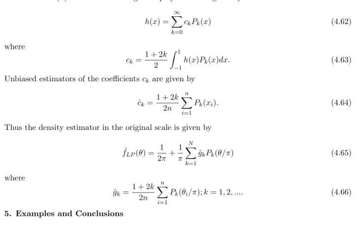
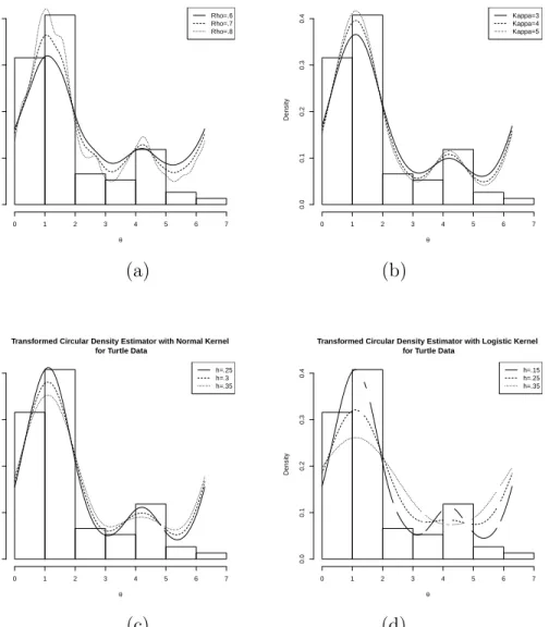
In this section we illustrate some of the density estimators by considering the wellknown Turtle data and Ants data. The Turtle data set gives the measurements of the directions taken by 76 turtles after treatment that is available from Appendix B.3 in Fisher (1993), whereas the Ants data set gives the measurements of the directions chosen by 100 ants in response to an evenly illuminated black target that is available from Appendix B.7 in Fisher (1993).
Figure 5.1 gives plots of the histogram with superimposed density estimators based on the wrapped Cauchy kernel and the von Misses kernel along with the transformed kernel estimators based on the classical kernel estimators based on Gaussian and logistic kernels for different values of the concentration and variance parameters, for Turtle data and Figure 5.2 presents the same for the Ants data. The kernel estimator for the transformed data on the real line is obtained from (1.3) where for the normal kernel
K(u) = √1
2πe
−1
2u 2
and that for the logistic kernel
K(u) = e
−u
Wrapped Cauchy Circular Density Estimators for Turtle Data
θ Density 0 1 2 3 4 5 6 7 0.0 0.1 0.2 0.3 0.4 Rho=.6Rho=.7 Rho=.8
von Mises Circular Kernel Density Estimators for Turtle Data
θ Density 0 1 2 3 4 5 6 7 0.0 0.1 0.2 0.3 0.4 Kappa=3Kappa=4 Kappa=5 (a) (b)
Transformed Circular Density Estimator with Normal Kernel for Turtle Data
θ Density 0 1 2 3 4 5 6 7 0.0 0.1 0.2 0.3 0.4 h=.25h=.3 h=.35
Transformed Circular Density Estimator with Logistic Kernel for Turtle Data
θ Density 0 1 2 3 4 5 6 7 0.0 0.1 0.2 0.3 0.4 h=.15h=.25 h=.35 (c) (d)
Figure 5.1: Histogram and Circular Kernel Density Estimators for Turtle data (a) Wrapped Cauchy kernel, ρ=.6, .7, .8.; (b) von Mises kernel, κ= 3,4,5.; (c) Transformed linear kernel with Gaussian kernel, h=.25, .3, .35.;
Wrapped Cauchy Circular Density Estimators for Ants Data
θ Density 0 1 2 3 4 5 6 7 0.0 0.1 0.2 0.3 0.4 0.5 Rho=.81Rho=.82 Rho=.83
von Mises Circular Kernel Density Estimators for Ants Data
θ Density 0 1 2 3 4 5 6 7 0.0 0.1 0.2 0.3 0.4 0.5 Kappa=5Kappa=6 Kappa=7 (a) (b)
Transformed Circular Density Estimator with Normal Kernel for Ants Data
θ Density 0 1 2 3 4 5 6 7 0.0 0.1 0.2 0.3 0.4 0.5 h=.2h=.25 h=.3
Transformed Circular Density Estimator with Logistic Kernel for Ants Data
θ Density 0 1 2 3 4 5 6 7 0.0 0.1 0.2 0.3 0.4 0.5 h=.15h=.25 h=.35 (c) (d)
Figure 5.2: Histogram and Circular Kernel Density Estimators for Ants data (a) Wrapped Cauchy kernel, ρ=.81, .82, .83; (b) von Mises kernel, κ= 5,6,7.; (c) Transformed linear kernel with Gaussian kernel, h=.2, .25, .3.;
(d) Transformed linear kernel with logistic kernel, h=.15, .25, .35.
The von Mises kernel seems to provide smoother plots as compared to wrapped Cauchy, however, both the kernels provide similar estimators, qualitatively. The estimators obtained by IS transfor-mation also produce similar results as to those given by the circular kernel estimators. Smoothing parameter may be selected using the proposal described in Taylor (2008). An enhanced strategy is to investigate a range of values around the value given by cross-validation.
5.2 Conclusions
This paper provides a simple approximation result for continuous function on defined on a unit circle to motivate circular kernel density estimator. An interesting connection between this estima-tor using the wrapped Cauchy kernel and an orthogonal series estimaestima-tor is discovered that shows
that truncation in the orthogonal series estimator may be avoided by using the wrapped Cauchy kernel. The approximation result used here also provides circular density estimator as the deriva-tive of smooth distribution function estimator. Some further families of estimators are suggested using stereographic projection of circle on different intervals that might provide easily computable estimators from well known software. Further studies about the estimators and their properties is being carried out in ongoing research investigation of the author.
References
Babu, G. J., Canty, A. and Chaubey, Y. P. (2002). Application of Bernstein polynomials for smooth estimation of a distribution and density function.J. Statist. Plann. Inference ,105, 377-392. Babu, G. J., and Chaubey, Y. P. (2006). Smooth estimation of a distribution and density function on
hypercube using Bernstein polynomials for dependent random vectors.Statistics and Probability Letters,76, 959-969.
Buckland, S. T. (1992). Fitting density functions with polynomials. J. R. Stat. Soc.,A41, 6376. Carnicero, J. A., Wiper, M. P. and Aus´ın, M. C. (2010). Circular Bernstein polynomial
distri-butions. Working Paper 10-25, Statistics and Econometrics Series 11, Departamento de Estad-stica Universidad Carlos III de Madrid. e-archivo.uc3m.es/bitstream/handle/10016/8318/ ws102511.pdf?sequence=1
ˇ
Cencov, N. N. (1962). Evaluation of an unknown distribution density from observations. Soviet Math. Dokl.,3, 1559-1562.
ˇ
Cencov, N. N. (1980). Statistical Decision Rules and Optimum Inference. New York: Springer-Verlag.
Chaubey, Y. P. (2016). Smooth Kernel Estimation of a Circular Density Function: A Connection to Orthogonal Polynomials on the Unit Circle.Preprint,https://arxiv.org/abs/1601.05053
Chaubey, Y.P.; Li, J.; Sen, A. and Sen, P. K. (2012). A new smooth density estimator for non-negative random variables.Journal of the Indian Statistical Association,50, 83-104.
Devroye, L. and Gy¨orfi, L. (1985). Nonparametric Density Estimation: The L1 View. New York: John Wiley & Sons
Di Marzio, M., Panzera, A., Taylor, C.C. (2009). Local Polynomial Regression for Circular Predic-tors.Statistics & Probability Letters,79(19), 2066–2075.
Di Marzio M, Panzera A, Taylor C. C. (2011). Kernel density estimation on the torus. Journal of Statistical Planning & Inference,141, 2156-2173.
Efromvich, S. (1999). Nonparametric Curve Estimation: Methods, Theory, and Applications, New York: Springer.
Efromvich, S. (2010). Orthogonal series density estimation. Wiley Interdisciplinary Rreviews, 2, 467-476.
E˘gecio˘glu, ¨Omer and Srinivasan, Ashok (2000). Efficient nonparametric density estimation on the sphere with applications in fluid mechanics. Siam J. Sci. Comput.22 152-176.
Fisher, N. I. (1989). Smoothing a sample of circular data, J. Structural Geology,11, 775–778. Fisher, N. I. (1993). Statistical Analysis of Circular Data.Cambridge University Press, Cambridge. Hall, P. (1980). Estimating a density on the positive half line by the method of orthogonal series.
Ann. Inst. Stat. Math.32, 351362.
Hall, P. (1981). On trigonometric series estimates of densities.Ann. Stat. 9, 683685. Hart, J. D. (1997). Nonparametric Smoothing and Lack-of-Fit Tests.New York: Springer.
Koornwinder, T. H., Wong, R. S. C., Koekoek, R., and Swarttouw, R.F. (2010). Orthogonal poly-nomials. InNIST Handbook of Mathematical Functions, Eds: Olver, Frank W. J.; Lozier, Daniel M.; Boisvert, Ronald F.; Clark, Charles W., London: Cambridge University Press.
Mhaskar, H. N. and Pai, D. V. (2000). Fundamentals of approximation Theory. Narosa Publishing House, New Delhi, India.
Parzen, E. (1962). On Estimation of a Probability Density Function and Mode.Ann. Math. Statist, 33:3, 1065-1076.
Prakasa Rao, B. L. S. (1983). Non Parametric Functional Estimation. Academic Press, Orlando, Florida.
Rudin, W. (1976).Real and Complex Analysis- Third Edition. McGraw Hill: New York.
Rudzkis, R. and Radavicius, M. (2005). Adaptive estimation of distribution density in the basis of algebraic polynomials. Theory Probab Appl,49, 93109.
Rosenblatt, M. (1956). Remarks on some nonparametric estimates of a density function.Ann. Math. Stat.,27:56, 832837
Simon, B. (2005). Orthogonal Polynomials on the Unit Circle, Part 1: Classical Theory. American Mathematical Society, Providence, Rhode Island.
Silverman B. W. (1986). Density Estimation for Statistics and Data Analysis. London: Chapman & Hall.
Tarter, M. E. and Lock, M. D. (1993).Model-Free Curve Estimation.New York: Chapman & Hall. Taylor, C. C. (2008). Automatic Bandwidth Selection for Circular Density Estimation.
Computa-tional Statistics & Data Analysis,52(7), 3493–3500.
Trefthen, L. N. (2013). Approximation Theory and Approximation Practice. SIAM: Philadelphia Vitale, R. A. (1973). A Bernstein polynomial approach to density estimation. Commun Stat, 2,
Walter, G. G. (1977). Properties of Hermite series estimation of probability density. Ann. Stat.,5, 12581264.
Walter, G. G. (1994). Wavelets and other Orthogonal Systems with Applications. London: CRC Press.