Understanding the role of sea surface
temperatureforcing for variability in global
temperature and precipitation extremes
Article
Published Version
Creative Commons: AttributionNoncommercialNo Derivative Works 4.0
Open Access
Dittus, A. J., Karoly, D. J., Donat, M. G., Lewis, S. C. and
Alexander, L. V. (2018) Understanding the role of sea surface
temperatureforcing for variability in global temperature and
precipitation extremes. Weather and Climate Extremes, 21. pp.
19. ISSN 22120947 doi:
https://doi.org/10.1016/j.wace.2018.06.002 Available at
http://centaur.reading.ac.uk/78154/
It is advisable to refer to the publisher’s version if you intend to cite from the
work. See
Guidance on citing
.
To link to this article DOI: http://dx.doi.org/10.1016/j.wace.2018.06.002
Publisher: Elsevier
All outputs in CentAUR are protected by Intellectual Property Rights law,
including copyright law. Copyright and IPR is retained by the creators or other
copyright holders. Terms and conditions for use of this material are defined in
the
End User Agreement
.
www.reading.ac.uk/centaur
CentAUR
Central Archive at the University of Reading
Reading’s research outputs online
Contents lists available atScienceDirect
Weather and Climate Extremes
journal homepage:www.elsevier.com/locate/wace
Understanding the role of sea surface temperature-forcing for variability in
global temperature and precipitation extremes
Andrea J. Dittus
a,b,c,∗, David J. Karoly
a,b, Markus G. Donat
b,d, Sophie C. Lewis
b,e,
Lisa V. Alexander
b,daSchool of Earth Sciences, The University of Melbourne, Parkville, Victoria, Australia bAustralian Research Council Centre of Excellence for Climate System Science, Australia cSchool of Earth, Atmosphere and Environment, Monash University, Clayton, Victoria, Australia dClimate Change Research Centre, UNSW Sydney, New South Wales, Australia
eSchool of Physical Environmental and Mathematical Sciences, University of New South Wales, Canberra, ACT, Australia
A B S T R A C T
The oceans are a well-known source of natural variability in the climate system, although their ability to account for inter-annual variations of temperature and precipitation extremes over land remains unclear. In this study, the role of sea-surface temperature (SST)-forcing is investigated for variability and trends in a range of commonly used temperature and precipitation extreme indices over the period 1959 to 2013. Using atmospheric simulations forced by observed SST and sea-ice concentrations (SIC) from three models participating in the Climate of the Twentieth Century Plus (C20C+) Project, results show that oceanic boundary conditions drive a substantial fraction of inter-annual variability in global average temperature extreme indices, as well as, to a lower extent, for precipitation extremes. The observed trends in temperature extremes are generally well captured by the SST-forced simulations although some regional features such as the lack of warming in daytime warm temperature extremes over South America are not reproduced in the model simulations. Furthermore, the models simulate too strong increases in warm day frequency compared to observations over North America. For extreme precipitation trends, the accuracy of the simulated trend pattern is regionally variable, and a thorough assessment is difficult due to the lack of locally significant trends in the observations. This study shows that prescribing SST and SIC holds potential predictability for extremes in some (mainly tropical) regions at the inter-annual time-scale.
1. Introduction
It is well known that the oceans are major drivers of internal climate variability, affecting climate around the globe (e.g. Shukla, 1998). Many modes of climatic variability are coupled ocean-atmosphere phenomena, such as the El Niño-Southern Oscillation (ENSO), which is the most important mode of variability for global climate on inter-an-nual timescales (e.g.McPhaden et al., 2006). The occurrence of an El Niño episode affects many regions worldwide through atmospheric teleconnections and increases global average temperatures in that year (e.g. Trenberth et al., 2002). ENSO also affects temperature and pre-cipitation extremes in many regions across the world (Kenyon and Hegerl, 2008,2010; Alexander et al., 2009; Arblaster and Alexander, 2012). Local SSTs can also be important for regional climate, for ex-ample, a recent study showed that SSTs to the northeast of Australia could enhance or dampen the ENSO-rainfall response in south-eastern Australia (van Rensch et al., 2015).
On a global scale, an example where natural variability in the Pacific Ocean is thought to have played an important role for global climate is through the so-called“hiatus” or slowdown in the rate of
increase in global mean surface temperature (GMST). Studies have shown that the hiatus may have been driven by low-frequency internal variability in the Pacific Ocean (Kosaka and Xie, 2013), associated with the negative phase of the Interdecadal Pacific Oscillation (Meehl et al., 2014; Watanabe et al., 2014) or prolonged La Niña-like conditions (Kosaka and Xie, 2013). This phase of the IPO is characterised by stronger trade winds (e.g.England et al., 2014) and cooler than normal sea-surface temperatures in the eastern Pacific, which have increased heat uptake by the oceans and thus contributed to the hiatus (Meehl et al., 2011).
While it is clear that natural variability in the oceans greatly in-fluences global climate in different ways, to date, few studies have systematically investigated the role of SST variability for temperature and precipitation extremes on land and their representation in global atmospheric climate models. Donat et al. (2016) compared century-long SST-driven runs from one atmospheric GCM with gridded ob-servations and reanalysis data. They found that SST variability could explain about 50% of the inter-annual variability of globally averaged temperature extremes and about 15% for precipitation extremes. Re-gionally, significant correlations between SST-driven runs and
https://doi.org/10.1016/j.wace.2018.06.002
Received 2 August 2017; Received in revised form 4 May 2018; Accepted 8 June 2018
∗Corresponding author. Now at: NCAS-Climate, Department of Meteorology, University of Reading, Reading, UK.
E-mail address:[email protected](A.J. Dittus).
Weather and Climate Extremes 21 (2018) 1–9
Available online 09 June 2018
2212-0947/ © 2018 The Authors. Published by Elsevier B.V. This is an open access article under the CC BY-NC-ND license (http://creativecommons.org/licenses/BY-NC-ND/4.0/).
observations were mainly found in the Tropics. However, under-standing and estimating internal variability is equally important to understanding the role of anthropogenic forcing, as it is a combination of both that drives climatic events in the real world. Climate variability can act to temporarily enhance (e.g. heatwaves in Australia during El Niño) or dampen (e.g. GMST hiatus) the effects of a warming climate. In this study, the potential of atmospheric simulations forced by observed SST and SIC conditions for understanding variability in temperature and precipitation extremes is investigated. Unlike in coupled ocean-atmosphere general circulation models (CGCMs), these atmospheric simulations will, by definition, have coupled ocean-atmosphere modes of variability in phase with the“real world”climate. Hence, there is potential for atmospheric simulations to be able to reproduce the timing of specific features of natural variability that coupled models may not. In this study, a multi-model ensemble of atmospheric simulations coordinated through the CLIVAR Climate of Twentieth Century Plus Project (Folland et al., 2014) and an observational dataset of extreme indices are used to assess the effect of SST-forcing in a suite of widely used indices of temperature and precipitation extremes. First, the effect of SST-forcing for inter-annual variability in the global land average of the temperature and precipitation extremes is assessed. The contribu-tion of SST-forcing to inter-annual variability is then quantified at the grid box level. Next, the relationship with ENSO is investigated in ob-servations and models. Finally, long-term trends in obob-servations and climate models are compared, to identify if prescribing SSTs and SIC improves the agreement between observed and modelled trends com-pared to coupled models. The paper is structured as follows. Section2 provides an overview of the extremes indices, data and methods used in this study. Results are shown in section 3, and potential applications and limitations of this study are discussed in section4. The conclusions of this paper are summarised in Section5.
2. Data and methods 2.1. Extreme indices
The extreme indices used in this paper are a subset of the 27 indices recommended by the Expert Team of Climate Change Detection and Indices (e.g.Zhang et al., 2011). Here, we exclude absolute threshold indices (such as e.g. the number of frost days or summer days) and duration indices, as we focus on indices that are meaningful across the globe. The 11 remaining indices are either relative threshold indices (i.e. percentile-based indices) or indices of annual maxima or minima. Additionally, we have added a normalized heavy precipitation index (R95pTOT) where the amount of heavy precipitation is normalized by the total precipitation at each grid box. This ensures that values from all grid boxes are comparable, rather than being dominated by regions of high precipitation. This index is used inFig. 1(global averages), while the subsequent figures are all using the heavy precipitation amount (R95p). These indices are summarised in Table 1. Note that some of these indices measure relatively “moderate” extremes, as they occur several times per year by definition in the case of the percentile indices. 2.2. Data
The observational data in this study were obtained from the GHCNDEX dataset (downloaded in February 2015;Donat et al., 2013). GHCNDEX was chosen for its length of record compared to other similar datasets, to better match the time period available in model simula-tions. Three global climate models contributing to the C20C+ project with various ensemble sizes are analysed in this study. The CAM5-1-1degree model (Neale et al. 2012) provides the largest ensemble with 50 simulations available from 1959 while for MIROC5 (Watanabe et al. 2010) and ACCESS1.3 (Bi et al., 2013), 10 and 5 runs were available respectively. These simulations are available for the period from 1959, 1950 and 1955 to 2013 or 2014 respectively, and cover a common
period from 1959 to 2013. The ACCESS1.3 and CAM5-1-1degree si-mulations were forced with observed SSTs and sea-ice (SICs) from the Hurrell et al. (2008)dataset. MIROC5 employed the Hadley Centre Sea Ice and Sea Surface Temperature data set (Rayner et al., 2003) as their forcing dataset. These historical simulations include natural and an-thropogenic forcings: solar and volcanic forcings (natural), greenhouse gas forcings (including CO2, N2O, CH4, and major CFCs), ozone,
sul-phate aerosols, black and organic carbon. An exception is the CAM5-1-1degree ensemble, which does not include volcanic forcings. Note that these models were the only ones available in the C20C+ archive at the time of analysis (December 2016), but more have been added since. However, the models analysed all belong to different ‘families’ of models (Knutti et al., 2013) and hence we estimate that this sub-en-semble is reasonably good to ensure sampling of structurally different models.
3. Methods
The required ETCCDI indices were calculated using the climdex.p-cic.ncdf R package provided by the Pacific Climate Impacts Consortium, Canada (https://github.com/pacificclimate/climdex.pcic.ncdf). This is the same software that was used to calculate the ETCCDI indices for CMIP5 models produced by the Canadian Community Climate Modelling Centre used in other studies (Sillmann et al., 2013), and required daily maximum and minimum temperature and precipitation data. This ensures that there are no methodological differences between the indices calculated here and the CMIP5 indices used in other studies. All indices were calculated on the models’native grid, and subsequently re-gridded to a common grid for the purposes of this study as described further down.
In a large enough ensemble, the ensemble mean represents the forced response to external forcings and prescribed boundary condi-tions such as greenhouse gases, aerosol, volcanic and solar forcings as well as SSTs and SIC in the model configuration of the C20C+ en-semble. The differences of the individual ensemble members from the ensemble mean therefore correspond to unforced atmospheric varia-bility, since the forced response is accounted for in the ensemble mean. However, in anyfinite ensemble, some residual unforced variability may remain in the ensemble mean.
As we are primarily interested in the forced component of inter-annual variability rather than long-term forcing, wefirst remove the linear trend from the time series for all analysis with the exception of section 3.3 on trends and where stated otherwise (e.g. Fig. 1). Re-moving this long-term trend also likely removes some long-term effects of solar and volcanic forcings and some decadal variability. The inter-annual variability in the de-trended time series is then primarily due to volcanic forcing and SST variability, or stochastic atmospheric varia-bility. Major volcanic eruptions in the second half of the Twentieth Century include Mt Agung in 1963, El Chichón in 1982, Pinatubo in 1991. Unless stated otherwise, the term“forced response”in this study refers to the forced component of inter-annual variability and not long-term forcing. The “common variance” across ensemble members is measured as the variance in the de-trended ensemble mean divided by the variance of a single de-trended ensemble member. Specifically, at each gridbox the ensemble member with the median variance in the ensemble is used, although the choice of the ensemble member has little overall effect on the results. The“fraction of common variance”can be interpreted as the fraction of variability forced by oceanic boundary conditions relative to stochastic atmospheric variability.
The model-simulated temperature and precipitation extremes were re-gridded to the resolution of the GHCNDEX observational dataset (2.5° × 2.5°) for all analyses using afirst order conservative remapping scheme and masked to the available observational coverage when cal-culating global averages. Only grid boxes where GHCNDEX contained valid data for at least 80% of all years were considered to minimise possible bias from too incomplete time series. Note the same masking
A.J. Dittus et al. Weather and Climate Extremes 21 (2018) 1–9
Fig. 1.Global land average time series of each of the 11 annual indices considered here, in order from left to right and top-to-bottom: cool nights, warm nights, cool days, warm days, hottest day, coldest day, coldest night, hottest night, contribution of very wet days to total precipitation, max. 5-day precipitation amount, max. 1-day precipitation amount. Observations are shown in red, each model ensemble is shown in a different colour. The correlation coefficient between the de-trended observations and individual ensemble members are given in the top right-hand corner. The correlation coefficient isfirst calculated for each ensemble member then averaged across all ensemble members of a single model, then across all models. The second number (“RensM”) corresponds to the correlation coefficient calculated
between observations and each model's ensemble mean, then averaged across all three models. (For interpretation of the references to colour in thisfigure legend, the reader is referred to the Web version of this article.)
A.J. Dittus et al. Weather and Climate Extremes 21 (2018) 1–9
and completeness criteria apply for the pattern correlations calculated inFigs. 3 and 4. Trends were calculated using a modified least squares method as outlined in the Intergovernmental Panel on Climate Change Fifth Assessment Report Supplementary Material (Hartmann et al., 2013), taking into account lag-1 autocorrelation in the residuals. Sta-tistical significance was assessed at the 5% level throughout this study, and adjusted for multiple hypothesis testing issues using the “false discovery rate”followingWilks (2016)and using a control level of 0.1 (i.e. double the statistical significance level used), as recommended by Wilks (2016) for spatially correlated data. For climate model data, black stippling indicates areas where at least 80% of realisations agree on sign and at least 50% are statistically significant using the criteria described above, while gray stippling indicates where observations lie within the model range. Finally, please note that the Niño3.4 index was calculated from theHurrell et al. (2008)SST dataset. All analysis was performed for calendar years from January to December, due to some precipitation indices currently only being available for the calendar year.
4. Results
The results are divided into three subsections. First, the ability of the atmospheric model simulations to reproduce observed year-to-year variability in the global land average of temperature and precipitation extremes is assessed. Then, the relationship of the extreme indices with ENSO is investigated. Finally, modelled and observed trend patterns are compared and key differences discussed.
4.1. Evaluation of global average temperature and precipitation extremes By prescribing the oceanic part of natural variability, atmospheric simulations are expected to capture some of the observed variability that coupled models may not. The simulations from all the models used in this study reproduce reasonably well the inter-annual variability of globally averaged annual percentage of warm days and nights, and cool days and nights (Fig. 1), with the average Spearman correlation coef-ficient between the de-trended observations and individual ensemble members ranging from 0.49 to 0.70. While in years with major volcanic eruptions the agreement between models and observations is nearly perfect (as expected), additional inter-annual agreement between ob-servations and models stems from prescribing the state of the ocean. Inter-annual agreement with observations is generally higher than for coupled models, as coupled models do include volcanic eruptions but generate their own internal variability (not shown). The hottest day and night of the year as well as the coolest night of the year (Fig. 1, panels 5 and 7–8) show lower but nevertheless statistically significant (p < 0.05) agreement in their year-to-year variability (with correla-tions between 0.35 and 0.41), while there is little agreement for the coolest day of the year (average correlation 0.17). All of the absolute
temperature indices show large temperature biases in all models. Note that the percentile indices by definition remove the model biases (since they are exceedances of percentile thresholds calculated from the model, rather than absolute or observed thresholds), which explains their better agreement with observations compared to the absolute in-dices. Most of the precipitation indices show little year-to-year varia-bility that is shared between observations and climate model simula-tions and show large biases, except for R95pTOT due to being normalized with total precipitation at each gridbox. Note however that the correlation coefficients are slightly higher for the R95p index (i.e. heavy precipitation above the 95th percentile, that is not normalized with total precipitation at each gridbox), since the global average of this precipitation index is dominated by regions of high total precipitation such as the tropics (R = 0.21, RensM = 0.30, not shown). It is further worth noting that the correlation coefficients between observations and the model mean (“RensM”inFig. 1, all de-trended) are systematically larger than the correlation coefficients averaged across individual en-semble members, which is not surprising since unforced atmospheric variability is averaged out in the ensemble mean. It is therefore not surprising that correlation coefficients are higher using the ensemble mean than when first calculated on each model realisation prior to averaging.
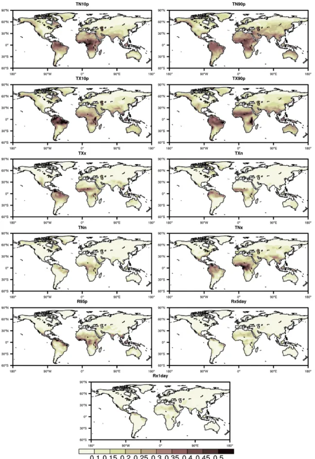
The fraction of“common variance” across ensemble members re-presents the fraction of the total variance (as represented by the var-iance of a single ensemble member) that is common to all ensemble members (i.e. variance of the ensemble mean). The“common variance” thus represents the fraction of variability that is found in all ensemble members and is likely forced by common boundary conditions, pri-marily SSTs and SIC but also including volcanic aerosols (except in the case of CAM, which does not include volcanoes) and solar forcing. The remainder represents unforced atmospheric variability that may be different in each ensemble member but averaged out in the ensemble mean. The fraction of common inter-annual variance (after de-trending) to all ensemble members is shown for each index for the CAM5-1-1degree model in Fig. 2. This model was chosen because it has the largest number of ensemble members available and results are thus more robust than those based on smaller ensembles. The results are very similar for the other models, with slightly larger fractions occur-ring outside the tropics, likely due to the smaller number of ensemble members used to produce the ensemble mean. The variance common to all ensemble members is largest for the percentile temperature indices, and is highest in the tropics where the fraction of SST-forced variance can reach up to 50 percent. SST forcing is also important for variability in the absolute temperature indices, although the common variance is lower for these extremes. There is some influence of SST-forcing on very wet days, but little to no influence on the annual wettest one andfi ve-day events. When analysed at a grid box level, the highest values of “common variance”are found in the tropics for all indices (Fig. 2). For the precipitation indices in particular, the common variance outside of Table 1
Definitions of extremes indices used in this study, followingZhang et al. (2011). Note that all indices except R95p and R95pTOT are also available on a monthly basis, but only annual indices are used here.
ID Name Definition Units
TN10p Cool Nights Annual percentage of days when daily min temperature < 10th percentile % TN90p Warm Nights Annual percentage of days when daily min temperature > 10th percentile % TX10p Cool Days Annual percentage of days when daily max temperature < 10th percentile % TX90p Warm Days Annual percentage of days when daily max temperature > 10th percentile % TXx Max Tmax Annual maximum value of daily max temperature °C TNx Max Tmin Annual maximum value of daily min temperature °C TXn Min Tmax Annual minimum value of daily max temperature °C TNn Min Tmin Annual minimum value of daily min temperature °C R95p Very wet days Annual total precipitation from days > 95th percentile mm R95pTOT Contribution of very wet days to total precipitation Fraction of annual total precipitation from days > 95th percentile unitless Rx1day Max 1-day precipitation amount Annual maximum 1-day precipitation mm Rx5day Max 5-day precipitation amount Annual maximum 5-day precipitation mm
A.J. Dittus et al. Weather and Climate Extremes 21 (2018) 1–9
Fig. 2.The fraction of common variance across 50 CAM5-1-1degree simulations is shown at the grid box level for all indices considered in this study. The fraction of common variance is calculated as the de-trended variance of the ensemble mean divided by the de-trended variance of a single ensemble member. At each grid box, the variance of the ensemble member with the median variance was used.
A.J. Dittus et al. Weather and Climate Extremes 21 (2018) 1–9
the tropics drops offrapidly, which is in line with the earlier observa-tion that the correlaobserva-tions between model-simulated heavy precipitaobserva-tion and observations are greater for the R95p index, which is dominated by high-rainfall areas, than R95pTOT, where all grid boxes contribute equally. Note that the assumption that other forcings are negligible is justified, since the“common variance”between ensemble members of a
coupled model is close to zero everywhere (not shown). 4.2. Relationship with ENSO
Next, the effects of ENSO on the variability in the extreme indices and their representation in the C20C+ ensemble are investigated. Fig. 3.Spearman correlation coefficient between de-trended percentage of warm days (top) and fraction of total precipitation from extreme precipitation (bottom) with Niño3.4 at each grid box. Thefigures on the top left are the correlation coefficients from the observations with Niño3.4, the remaining panels represent the average correlation coefficients for each model with Niño3.4. Statistical significance was calculated for each individual ensemble member at the 5% level and adjusted for the effects of multiple hypothesis testing using the false discovery rate followingWilks (2016). Black stippling indicates areas where at least 80% of available realisations agree on sign and 50% are statistically significant. In other words, black stippling indicates significance and robustness among model simu-lations. Gray (larger) stippling indicates that observations lie within the model range, i.e. model simulations are consistent with observations. Gray hatching indicates that models are not consistent with observations, while absence of gray stippling/hatching indicates that observations are not available. The average pattern correlation coefficients between the modelled and the observed patterns are given in the bottom left of each panel. Again, pattern correlations were calculated for each realisation and subsequently averaged.
A.J. Dittus et al. Weather and Climate Extremes 21 (2018) 1–9
ENSO being the most important coupled atmosphere-ocean mode of variability on inter-annual timescales, it is likely that the year-to-year variability of temperature and precipitation extremes in some regions is influenced by ENSO, as has previously been shown in observational and modelling studies (e.g. Kenyon and Hegerl, 2008, 2010; Alexander et al., 2009;Arblaster and Alexander, 2012).
The correlation coefficients between the Niño3.4 index and the
annual number of warm days as well as precipitation on very wet days respectively are shown inFig. 3 for the average of the correlations calculated for each ensemble member individually. We only show one temperature index and one precipitation index here for better read-ability, additional indices can be found in theSupplementary Material (S1-S9).
The simulations reproduce the positive correlation between warm Fig. 4.Linear trends in observations and the average trend in each model for the percentage of warm days (top) and precipitation exceeding the 95th percentile (bottom). In the observations, significant trends at the 5% level are stippled, adjusted using the false discovery rate method followingWilks (2016)as above. For the models, black stippling indicates areas where 80% of all realisations agree on sign and at least 50% are statistically significant at the 5% level. In other words, black stippling indicates significance and robustness among model simulations. Gray (larger) stippling indicates that observations lie within the model range, i.e. model simulations are consistent with observations. Gray hatching indicates that models are not consistent with observations, while absence of gray stippling/hatching indicates that observations are not available. Pattern correlations werefirst calculated for each ensemble member then averaged across all members of a single model.
A.J. Dittus et al. Weather and Climate Extremes 21 (2018) 1–9
temperature extremes and Niño3.4 in north-western North America, and the corresponding negative correlation coefficients in south-eastern North America (Fig. 3). Black stippling over these areas in the models indicates that this is a robust model response across different ensemble members. They further also simulate the correct sign over Australia and south-east Asia, which indicate an increase in warm days during El Niño conditions, although the correlations are too weak in the models over Australia.
Furthermore, the models all show a strong and coherent positive correlation over northern South America including the Amazon region, however observations are not available over this region. The CAM5 model produces robust positive correlations between warm days and Niño3.4 over tropical latitudes of Africa, that are much weaker in the other models. Again, observations are not available over this region. A strong negative correlation in the Himalayas is found in the ACCESS model (and to a lesser extent in MIROC5) that is not seen in CAM5. Despite these differences, overall the model simulations reproduce the observed correlation pattern over the regions with observational cov-erage remarkably well, with pattern correlations between 0.51 and 0.59 depending on the model. Furthermore, the gray stippling indicates that where observations are available, the models are largely consistent with observations. The lesser consistency for MIROC5 and ACCESS1.3 compared to CAM5 is likely due to the reduced ensemble size. Note that these pattern correlations are calculated for each individual ensemble member then averaged, and are therefore smaller than if they were calculated on the average correlations directly (not shown).
For precipitation extremes, the pattern correlation of the ENSO-correlationfields is lower, ranging from 0.21 to 0.30 depending on the model. The models reproduce the correlation sign over Australia, the eastern coast of South America and Western Europe, albeit most of these local correlations are not statistically significant in either the observations or the climate models. All models show a negative corre-lation in the Amazonas region (albeit with different magnitudes and levels of statistical significance) and similar patterns of correlations over Africa, however observational data are not available in these re-gions. It is worth noting that the spatial pattern is much more hetero-geneous than for temperature extremes in both observations and models, and that most regions do not exhibit statistically significant correlations with Niño3.4. It is therefore not surprising that the pattern agreement between observed and modelled correlation coefficients is substantially lower than for temperature extremes. The gray stippling indicates that the simulated correlation coefficients are largely con-sistent with observations where they are available, confirming that the lack of pattern agreement is likely due to little impact of ENSO on annual rainfall from events exceeding the 95th percentile in many re-gions of the world, rather than poor model performance.
4.3. Trend patterns of temperature and precipitation extremes
Finally, this section examines whether regional trends in tempera-ture and precipitation extremes as simulated in the C20C+ ensemble can be better captured than in coupled climate model simulations. Again, only two temperature and precipitation indices are shown here, additional indices can be found in the Supplementary Material,Figures S10-18. The average trend across all ensemble members is shown here. The simulated trend patterns are broadly similar to the observed trends (pattern correlations≥0.78), with widespread increases in the frequency of warm days in both observations and models. However, there are also some marked differences, for example, the observations show an area of decreases in the frequency of warm days in parts of southern South America, which is not reproduced in any of the models (Fig. 4). This decrease in observed warm day frequency lies outside of the model range, indicating that the models are either biased or that the ensemble is not large enough to reflect the“true”unforced variability. Additionally, the simulated increase in warm day frequency over North America is very robust across the models but inconsistent with
observations over a large area of the United States. In this area, ob-servations show a weaker increase that is not statistically significant. Interestingly, all realisations (not shown) of all models show small areas of decreases in warm days in different locations of Asia that are not observed, albeit in different locations, which is likely associated with the response to aerosol forcing in this region in different models (see Fig. 4for the model average).
It is difficult to compare trends in the simulated precipitation ex-tremes with observations since trends in this variable are weak and the variability that is not SST-driven is large. Therefore, pattern correla-tions are close to zero, as expected, due to weak local trends that are not statistically different from zero. It is interesting to note that for most regions, observed trends lie within the model spread. Note however that studies have found that atmospheric simulations consistently pro-duced mean and extreme precipitation changes of the wrong sign over Australia and East Asia (Dong et al., 2017). Consistent with these stu-dies, trends in heavy precipitation of the opposite sign to the observa-tions (albeit not significant) are found over northern Australia in the ensemble mean for some models (Fig. 4). Furthermore, the pattern correlations for the precipitation extremes are substantially higher for the coupled MIROC5 model (up to 0.41 for R95p,Figure S19) than for the C20C+ models. Therefore, caution is strongly recommended when using AMIP-style simulations for the analysis of regional trends in precipitation extremes.
5. Discussion
The results presented in this study show that SST and SIC-forcing plays an important role for temperature and precipitation extremes. In particular, inter-annual variations of globally averaged percentile temperature indices and annual maximum and minimum temperatures are driven to a large extent by variability in SSTs. It is likely that the effect of SSTs, and ENSO in particular, affects extreme indices to dif-ferent extents in different seasons. Hence, by analysing annual indices of extremes and Niño3.4 we expect some of the signal to be smoothed out, especially as Niño3.4 SST anomalies usually switch sign during the first half of the calendar year. Nevertheless, this analysis shows that the climate models are able to broadly reproduce the pattern associated with the El Niño-Southern Oscillation in the observations. Although not shown here, an analysis of composites of climate extremes for El Niño and La Niña conditions separately has shown that the responses to ENSO are simulated similarly well for both phases.
Another important point to note is that the estimates provided in this study are likely to be conservative estimates of the influence of SSTs on temperature and precipitation extremes. For example, it is possible that local SSTs (e.g. unusually warm SSTs in a certain year) can be important for a particular event over a region, without this region necessarily showing a strong influence of SSTs or ENSO every year. This type of influence on individual events would not necessarily be picked up in this analysis. Nevertheless, this study identifies regions with po-tential“added predictability”compared to coupled models, stemming from the fact that oceanic boundary conditions are prescribed. Therefore, for regions where SSTs force a substantial part of atmo-spheric variability, atmoatmo-spheric model simulations might provide sub-stantial added value for investigating mechanisms or detection and attribution of specific events. However, as other studies have found, ocean-atmosphere coupling is particularly important for precipitation trends, and therefore these types of simulations may not be particularly suitable for detection and attribution of precipitation extremes. Our results however show that these simulations may be more valuable in particular for investigating variability and trends in temperature ex-tremes.
6. Conclusions
In this study, the influence of SST-forcing on inter-annual variations
A.J. Dittus et al. Weather and Climate Extremes 21 (2018) 1–9
and trends in eight temperature and three precipitation extremes is examined. Using atmospheric simulations from three climate models forced by observed SSTs and SIC, the respective roles of SST-forcing and stochastic atmospheric variability are assessed for global land averages of these extremes indices. For warm temperature extremes, SST-forcing drives a large portion of inter-annual variability, particularly in but not limited to the tropics. For annual precipitation extremes, the effect of SST-forcing on global average time series is smaller, and its influence is limited to the tropics, where in climate model simulations it can explain between 10 and 50% of the year-to-year variability in certain locations, depending on the index considered. The models used here are able to capture most key features in the relationship between ENSO and tem-perature and precipitation extremes.
Finally, our analysis shows no obvious improvement in SST-driven atmospheric models over coupled ocean-atmosphere models in the si-mulated regional trends in temperature extremes and suggests that the trends in precipitation extremes may agree less with observations in the C20C+ models than in coupled models. Regional details such as a decrease in the frequency of warm days over a region in southern South America are not simulated by the models, which suggests that either this observational feature is not forced by SST-variability, or that the models are unable to represent a process necessary to reproduce this feature. Since none of the ensemble members capture a cooling in this area, this would suggest a deficiency or missing process in the models. However, since the ensembles arefinite, it is equally possible that our ensembles may be too small to capture the ‘true’range of unforced variability. Similarly, the models are inconsistent with observations in large parts of North America, where the simulated increase in warm days is too strong compared to observations. The trend patterns in precipitation extremes are hard to assess in the absence of strong sta-tistically significant local trends in the observations. However, it is worth noting that in all model simulations, the sign of the trend over North America and Australia is opposite to that found in observations, which is reflected in pattern correlations close to zero. Pattern corre-lations from one coupled model suggest that this problem is worse in atmosphere-only simulations than in coupled model simulations. Acknowledgements
Authors are supported by Australian Research Council grant CE110001028. AJD also acknowledges the David Lachlan Hay Memorial Fund. SCL is supported by Australian Research Council Grant DE160100092. MGD is supported by Australian Research Council Grant DE150100456. LVA is supported by Australian Research Council Grant DP160103439.
Appendix A. Supplementary data
Supplementary data related to this article can be found athttps:// doi.org/10.1016/j.wace.2018.06.002.
References
Alexander, L.V., Uotila, P., Nicholls, N., 2009. Influence of sea surface temperature variability on global temperature and precipitation extremes. J. Geophys. Res. Atmos. 114https://doi.org/10.1029/2009JD012301.D18116.
Arblaster, J.M., Alexander, L.V., 2012. The impact of the El Niño-Southern Oscillation on maximum temperature extremes. Geophys. Res. Lett. 39https://doi.org/10.1029/ 2012GL053409.L20702.
Bi, D., et al., 2013. The ACCESS Coupled Model: Description, Control Climate and Evaluation. pp. 1–24.
Donat, M.G., Alexander, L.V., Yang, H., Durre, I., Vose, R., Caesar, J., 2013. Global
land-based datasets for monitoring climatic extremes. Bull. Am. Meteorol. Soc. 94, 997–1006.https://doi.org/10.1175/BAMS-D-12-00109.1.
Donat, M.G., Alexander, L.V., Herold, N., Dittus, A.J., 2016. Temperature and pre-cipitation extremes in century-long gridded observations, reanalyses, and atmo-spheric model simulations. J. Geophys. Res. Atmos. 121, 11174–11189.https://doi. org/10.1002/2016JD025480.
Dong, B., Sutton, R.T., Shaffrey, L., Klingaman, N.P., 2017. Attribution of forced decadal climate change in coupled and uncoupled ocean-atmosphere model experiments. J. Clim. 1–50.https://doi.org/10.1175/JCLI-D-16-0578.1.JCLI–D–16–0578. England, M.H., et al., 2014. Recent intensification of wind-driven circulation in the
Pacific and the ongoing warming hiatus. Nat. Clim. Change 4, 222–227.https://doi. org/10.1038/nclimate2106.
Folland, C., Stone, D., Frederiksen, C., Karoly, D.J., Kinter, J., 2014. The international CLIVAR climate of the 20th century Plus (C20C+) project: Report of the sixth workshop. CLIVAR Exch. 19, 57–59.
Hartmann, D.L., et al., 2013. Observations: atmosphere and surface supplementary ma-terial. Climate change 2013: the physical science basis. In: Stocker, T.F. (Ed.), Contribution of Working Group I to the Fifth Assessment Report of the Intergovernmental Panel on Climate Change.
Hurrell, J.W., et al., 2008. In: A New Sea Surface Temperature and Sea Ice Boundary Dataset for the Community Atmosphere Model, vol.21. pp. 5145–5153.https://doi. org/10.1175/2008JCLI2292.1. https://doi.org.ezproxy.lib.monash.edu.au/10. 1175/2008JCLI2292.1.
Kenyon, J., Hegerl, G.C., 2008. Influence of modes of climate variability on global tem-perature extremes. J. Clim. 21, 3872–3889.https://doi.org/10.1175/
2008JCLI2125.1.
Kenyon, J., Hegerl, G.C., 2010. Influence of modes of climate variability on global pre-cipitation extremes. J. Clim. 23, 6248–6262.https://doi.org/10.1175/
2010JCLI3617.1.
Knutti, R., Masson, D., Gettelman, A., 2013. Climate model genealogy: generation CMIP5 and how we got there. Geophys. Res. Lett. 40, 1194–1199.https://doi.org/10.1002/ grl.50256.
Kosaka, Y., Xie, S.-P., 2013. Recent global-warming hiatus tied to equatorial Pacific surface cooling. Nature 501, 403–407.https://doi.org/10.1038/nature12534. McPhaden, M.J., Zebiak, S.E., Glantz, M.H., 2006. ENSO as an integrating concept in
earth science. Science 314, 1740–1745.https://doi.org/10.1126/science.1132588. Meehl, G.A., Teng, H., Arblaster, J.M., 2014. Climate model simulations of the observed
early-2000s hiatus of global warming. Nat. Clim. Change 4, 898–902.https://doi. org/10.1038/nclimate2357.
Meehl, G.A., Arblaster, J.M., Fasullo, J.T., Hu, A., Trenberth, K.E., 2011. Model-based evidence of deep-ocean heat uptake during surface-temperature hiatus periods. Nat. Clim. Change 1, 360–364.https://doi.org/10.1038/nclimate1229.
Neale, R.B., Chen, C.C., Gettelman, A., Lauritzen, P.H., Park, S., Williamson, D.L., Conley, A.J., Garcia, R., Kinnison, D., Lamarque, J.F., Marsh, D., Mills, M., Smith, A.K., Tilmes, S., Vitt, F., Morrison, H., Cameron-Smith, P., Collins, W.D., Iacono, M.J., Easter, R.C., Ghan, S.J., Liu, X., Rasch, P.J., Taylor, M.A., 2012. Description of the NCAR Community Atmosphere Model (CAM 5.0). Technical Report; NCAR Technical Note NCAR/TN-486+STR..
Rayner, N., Parker, D.E., Horton, E.B., Folland, C.K., Alexander, L.V., Rowell, D.P., Kent, E.C., Kaplan, A., 2003. Global analyses of sea surface temperature, sea ice, and night marine air temperature since the late nineteenth century. J. Geophys. Res. 108, 4407. https://doi.org/10.1029/2002JD002670.
Shukla, J., 1998. Predictability in the midst of chaos: a scientific basis for climate fore-casting. Science 282, 728–731.
Sillmann, J., Kharin, V.V., Zhang, X., Zwiers, F.W., Bronaugh, D., 2013. Climate extremes indices in the CMIP5 multimodel ensemble: Part 1. Model evaluation in the present climate. J. Geophys. Res. Atmos. 118, 1716–1733.https://doi.org/10.1002/jgrd. 50203. http://onlinelibrary.wiley.com/doi/10.1002/jgrd.50203/full. Trenberth, K.E., Caron, J.M., Stepaniak, D.P., Worley, S., 2002. Evolution of El
niño–southern oscillation and global atmospheric surface temperatures. J. Geophys. Res. Atmosphere 107, 2044.https://doi.org/10.1029/2000JD000298.
van Rensch, P., Gallant, A.J.E., Cai, W., Nicholls, N., 2015. Evidence of local sea surface temperatures overriding the southeast Australian rainfall response to the 1997–1998 El Niño. Geophys. Res. Lett. 42, 9449–9456.https://doi.org/10.1002/
2015GL066319.
Watanabe, M., et al., 2010. Improved climate simulation by MIROC5: mean states, variability, and climate sensitivity. J. Clim. 23, 6312–6335.https://doi.org/10.1175/ 2010JCLI3679.1.
Watanabe, M., Shiogama, H., Tatebe, H., Hayashi, M., Ishii, M., Kimoto, M., 2014. Contribution of natural decadal variability to global warming acceleration and hiatus. Nat. Clim. Change 4, 893–897.https://doi.org/10.1038/nclimate2355. Wilks, D.S., 2016.“The stippling shows statistically significant grid points”: how Research
results are routinely overstated and overinterpreted, and what to do about it. Bull. Am. Meteorol. Soc. 97, 2263–2273.https://doi.org/10.1175/BAMS-D-15-00267.1. Zhang, X., Alexander, L., Hegerl, G.C., Jones, P., Tank, A.K., Peterson, T.C., Trewin, B.,
Zwiers, F.W., 2011. Indices for monitoring changes in extremes based on daily temperature and precipitation data. WIREs Clim Change 2, 851–870.https://doi.org/ 10.1002/wcc.147.
A.J. Dittus et al. Weather and Climate Extremes 21 (2018) 1–9