DOI 10.1007/s11263-016-0985-3
Dynamic Behavior Analysis via Structured Rank Minimization
Christos Georgakis1 · Yannis Panagakis1,2 · Maja Pantic1,3Received: 15 March 2016 / Accepted: 21 December 2016
© The Author(s) 2017. This article is published with open access at Springerlink.com Abstract Human behavior and affect is inherently a
dynamic phenomenon involving temporal evolution of pat-terns manifested through a multiplicity of non-verbal behav-ioral cues including facial expressions, body postures and gestures, and vocal outbursts. A natural assumption for human behavior modeling is that a continuous-time charac-terization of behavior is the output of a linear time-invariant system when behavioral cues act as the input (e.g., continu-ous rather than discrete annotations of dimensional affect). Here we study the learning of such dynamical system under real-world conditions, namely in the presence of noisy behav-ioral cues descriptors and possibly unreliable annotations by employing structured rank minimization. To this end, a novel structured rank minimization method and its scalable variant are proposed. The generalizability of the proposed framework is demonstrated by conducting experiments on 3 distinct dynamic behavior analysis tasks, namely (i) conflict intensity prediction, (ii) prediction of valence and arousal, and (iii) tracklet matching. The attained results outperform Communicated by Cordelia Schmid and Thomas Brox.
B
Christos Georgakis [email protected] Yannis Panagakis [email protected] Maja Pantic [email protected]1 Department of Computing, Imperial College London, 180 Queens Gate, London SW7 2AZ, UK
2 Department of Computer Science, Middlesex University, London, UK
3 Faculty of Electrical Engineering, Mathematics and Computer Science (EEMCS), University of Twente, Enschede, The Netherlands
those achieved by other state-of-the-art methods for these tasks and, hence, evidence the robustness and effectiveness of the proposed approach.
Keywords Dynamic behavior analysis·Structured rank minimization·Linear time-invariant systems ·Hankel matrix·Low-rank·Sparsity
1 Introduction
Analysis of human behavior concerns detection, tracking, recognition, and prediction of complex human behaviors including affect and social behaviors such as agreement and conflict escalation/resolution from audio-visual data cap-tured in naturalistic, real-world conditions. Modeling human behavior for automatic analysis in such conditions is the pre-requisite for next-generation human-centered computing and novel applications such as personalized natural interfaces (e.g., in autonomous cars), software tools for social skills enhancement including conflict management and negotia-tion, and assistive technologies (e.g., for independent living), to mention but a few.
Traditionally, research in behavior and affect analysis has focused on recognizing behavioral cues such as smiles, head nods, and laughter (Déniz et al. 2008; Kawato and Ohya 2000;Lockerd and Mueller 2002), pre-defined posed human actions (e.g., walking, running, and hand-clapping) (Dollár et al. 2005;Niebles et al. 2008;Georgakis et al. 2012) or dis-crete, basic emotional states (e.g., happiness, sadness) (Pantic and Rothkrantz 2000; Cohen et al. 2003; Littlewort et al. 2006) mainly from posed data acquired in laboratory settings. However, these models are deemed unrealistic as they are unable to capture the temporal evolution of non-basic, pos-sibly atypical, behaviors and subtle affective states exhibited by humans in naturalistic settings. In order to accommodate
such behaviors and subtle expressions, continuous-time and dimensional descriptions of human behavior and affect have been recently employed (Gunes and Pantic 2010;Gunes et al. 2011;Pantic et al. 2011;Pantic and Vinciarelli 2014;Vrigkas et al. 2015). For instance, the temporal evolution of level of interest (Nicolaou et al. 2014; Panagakis et al. 2016) and agreement (Bousmalis et al. 2011;Rakicevic etal. 2016), or the intensity of pain (Kaltwang et al. 2012, 2015) and con-flict (Kim et al. 2012a,b;Panagakis et al. 2016) is precisely described as continuous-valued function of time. In analogy, dimensional and continuous description of human emotion consists of characterizing emotional states in terms of a number of latent dimensions over time (Gunes et al. 2011). Two dimensions are deemed sufficient for capturing most of the affective variability: valence and arousal (V–A), signify-ing respectively, how positive/negative and active/inactive an emotional state isLane and Nadel(2002).
Representative machine learning models employed for automatic, continuous behavior and emotion analysis include Hidden Markov Models (HMMs) (Cohen et al. 2003) for facial expression recognition, Dynamic Bayesian Net-works (DBN) for human motion classification and track-ing (Pavlovi´c et al. 1999), Conditional Random Fields (CRFs) for prediction of visual backchannel cues (i.e., head nods) (Morency et al. 2010), Long-Short Term Mem-ory (LSTM) Neural Networks for continuous prediction of dimensional affect (Nicolaou et al. 2011), and regression-based approaches for continuous emotion and depression recognition or pain estimation (Nicolaou et al. 2012;Valstar et al. 2013;Kaltwang et al. 2012). Despite their merits, these methods rely on large sets of training data, involve learning of a large number of parameters, they do not model dynamics of human behavior and affect in an explicit way, and, more importantly, they are fragile in the presence of gross non-Gaussian noise and incomplete data, which is abundant in real-world (visual) data.
Contributions In this work, we model and tackle the problem ofdynamic behavior analysisin the presence of gross, but sparse noise and incomplete visual data under a different perspective, making the following contributions:
1. The modeling assumption here is that for smoothly-varying dynamic behavior phenomena, such as conflict escalation and resolution, temporal evolution of human affect described in terms of valence and arousal, or motion of human crowds, among others, the observed data can be postulated to be trajectories (inputs and out-puts) of a linear time-invariant (LTI) system. Recent advances in system theory (Van Overschee and De Moor 2012;Fazel et al. 2013) indicate that such dynamics can be discovered by learning a complexity (i.e.,
low-order) LTI system based on its inputs and outputs via rank minimization of a Hankel matrix constructed from the observed data. Here, continuous-time annotations char-acterizing the temporal evolution of relevant behavior or affect are considered as system outputs, while (visual) features describing behavioral cues are deemed system inputs. In practice, visual data are often contaminated by gross, non-Gaussian noise mainly due to pixel corrup-tions, partial image texture occlusions or feature extrac-tion failure (e.g., incorrect object localizaextrac-tion, tracking errors), and human assessments of behavior or affect may be unreliable mainly due to annotator subjectivity or adversarial annotators. The existing structured rank minimization-based methods perform sub-optimally in the presence of gross corruptions. Therefore, to robustly learn a LTI system from grossly corrupted data, we for-mulate a novelq-norm regularized (Hankel) structured Schatten- p norm minimizationproblem in Sect.3. The Schattenp- and the sparsity promotingq-norm act either as convex surrogates, whenp=q =1, or as non-convex approximations, whenp,q ∈(0,1), of the rank function and the0-(quasi) norm, respectively.
2. To tackle the proposed optimization problem, an algo-rithm based on the Alternating-Directions Method of Multipliers (ADMM) (Bertsekas 2014) is developed in Sect.4. Furthermore, in the same section a scalable ver-sion the algorithm is elaborated.
3. The proposed model is the heart of a general and novel framework for dynamic behavior modeling and analysis, which is detailed in Sect.5. A common practice in behav-ioral and affective computing is to train machine learning algorithms by employing large sets of training data that comprehensively cover different subjects, contexts, inter-action scenarios and recording conditions. The proposed approach allows us to depart from this practice. Specif-ically, we demonstrate for the first time that complex human behavior and affect, manifested by a single per-son or group of interactants, can be learned and predicted based on a small amount of person(s)-specific observa-tions, amounting to a duration of just a few seconds. 4. The effectiveness and the generalizability of the
pro-posed model is corroborated by means of experiments on synthetic and real-world data in Sect. 6. In par-ticular, the generalizability of the proposed framework is demonstrated by conducting experiments on 3 dis-tinct dynamic behavior analysis tasks, namely (i) con-flict intensity prediction, (ii)prediction of valence and arousal, and (iii)tracklet matching. The attained results outperform those achieved by other state-of-the-art meth-ods on both synthetic and real-world data and, hence, evidence the robustness and effectiveness of the proposed approach. The proposed framework is graphically illus-trated in Fig.1.
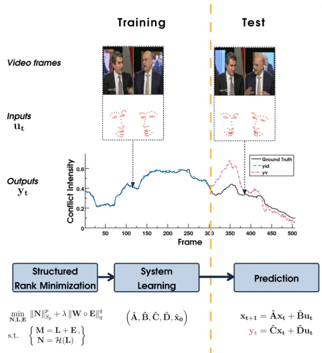
Fig. 1 Illustration of the proposed dynamic behavior analysis frame-work, as applied on the task of conflict intensity prediction for a sequence from CONFER dataset. A portion of the sequence frames
is used for LTI system learning through the proposed structured rank minimization method (training), while the remaining frames are used for prediction (test)
2 Background and Related Work
In this section, notation conventions and mathematical for-malism related to Hankel matrix structure are first introduced. Next, in order to make the paper self-contained, we describe how learning of dynamical systems and, in particular, of a LTI system can be cast as a (Hankel) structured rank minimization problem. Related works on structured rank minimization and their applications in visual information processing are also described.
2.1 Preliminaries
Notations Matrices (vectors) are denoted by uppercase (low-ercase) boldface letters, e.g.,X, (x).Idenotes the identity matrix of compatible dimensions. Theith element of vec-tor x is denoted as xi, the ith column of matrix X is denoted as xi, while the entry of X at position (i,j) is denoted by xi j. For the set of real numbers, the symbol R is used. For two matrices A and B in Rm×n, A◦ B denotes the Hadamard (entry-wise) product of A and B,
whileA,Bdenotes the inner product tr(ATB), where tr(·) is the trace of a square matrix. For a symmetric positive semi-definite matrixA, we write A 0. Regarding vec-tor norms,x := ixi2 denotes the Euclidean norm. The sign function is denoted by sgn(·), while| · | denotes the absolute value operator. Regarding matrix norms, the0
-(quasi-) norm, which equals the number of non-zero entries, is denoted by · 0.Xq := i
j|Xi j|q
1/q is the matrix q-norm, of which the Frobenius norm XF :=
i
j Xi j2 =
tr(XTX)is a special case whenq =2. X denotes the spectral norm, which equals the largest singular value. If σi(X) is the ith singular value of X,
XSp :=
iσi(X)p
1/p
is the Schatten p-norm ofX, of which the nuclear normX∗:=iσi(X)is a special case whenp=1. Linear maps are denoted by scripted letters. For a linear mapA:Rm×n→Rp,A∗denotes the adjoint map ofA, whileσmax(A)denotes the maximum singular value of
A.Idenotes the identity map.
The Hankel Matrix Structure LetA= [A0A1 . . . Aj+k−2] be am×n(j+k−1)matrix, with eachAtbeing am×n matrix fort = 0,1, . . . ,j +k−2. We define the Hankel linear mapH(A):=Hm,n,j,k(A), where
Hm,n,j,k(A)= ⎛ ⎜ ⎜ ⎜ ⎝ A0 A1· · · Ak−1 A1 A2· · · Ak ... ... ... ... Aj−1 Aj · · ·Aj+k−2 ⎞ ⎟ ⎟ ⎟ ⎠∈Rm j×nk, (1)
and∈Rnk×qwithσmax()≤1 (Fazel et al. 2013).
There-fore,Hm,n,j,k(A)is a block-Hankel matrix withj×kblocks, where eachAiis a matrix of dimensionm×n. Note that the Hankel structure enforces constant entries along the skew diagonals. We denote byT = j+k−1 the total number of observations, whileM =m j andN =nkdenote the num-ber of rows and columns of the Hankel matrixHm,n,j,k(A), respectively. For notational convenience, we writeH(A)to denoteHm,n,j,k(A), when the dimensionsm,n,j,kare clear from the context.
The adjoint mapH∗is defined asH∗()=H∗
m,n,j,k(T), where for any matrixB∈Rm j×nk
Hm∗,n,j,k(B)=Hm∗,n,j,k ⎛ ⎜ ⎜ ⎜ ⎝ B00 B01 · · · B0,k−1 B10 B11 · · · B1,k−1 ... ... ... ... Bj−1,0Bj−1,1· · ·Bj−1,k−1 ⎞ ⎟ ⎟ ⎟ ⎠ =B00 B01+B10. . . B02+B11+B20 · · · Bj−1,k−1 ∈Rm×n(j+k−1). (2)
It is proved inFazel et al. (2013) thatHm∗,n,j,k(B)2
F ≤
LB2F, whereL :=min{j,k}. This finding, combined with σmax()≤1, entails that the spectral norm of the adjoint map
H∗is less than or equal to√L. Herein, the space of Hankel matrices is denoted bySH.
2.2 LTI System Learning via Structured Rank Minimization
Dynamical systems, such as LTI systems, are able to com-pactly model the temporal evolution of time-varying data. While the dynamic model can be considered as known in some applications (e.g., Brownian dynamics in motion mod-els), it is in general unknown and, hence, should be learned from the available data.
Consider a sequence of observed outputs yt ∈ Rm and inputsut ∈ Rd, respectively, for t = 0, . . . ,T −1. The goal is to find from the observed data, a state-space model, corresponding to a LTI system, given by
xt+1=Axt+But yt=Cxt+Dut
(3)
such that the system is of low-order, i.e., it is associated with a low-dimensional state vectorxt ∈ Rn at timet, wheren is theunknowntrue system order. The order of the system (i.e., the dimension of the state vector) captures the memory of the system and it is a measure of its complexity. In (3), both the state and the measurement equations are linear and the parameters of the system, i.e., the matrices A,B,C,D are constant over time but their dimensions are unknown. Therefore, to determine the model, we need to find the model ordern, the matricesA,B,C,D, and the initial statex0. To this end, the model order should be estimated first. Next, the estimation of the system order using Hankel matrices is summarized.
Let us assume that the unknown state vectors has dimen-sionr >nand letX= [x0 x1 . . . xT−1] ∈Rr×T,Y=
[y0 y1 . . . yT−1] ∈Rm×T,U= [u0 u1 . . . uT−1] ∈ Rd×T be the matrices containing in their columns the unknown state vectors, the observed outputs, and the observed inputs of the system, respectively, fort =0,1, . . . ,T −1. Let alsoHm,1,r+1,T−r(Y)andHd,1,r+1,T−r(U)be the Han-kel matrices constructed from the observed system outputs and inputs, respectively, according to (1) andU⊥∈R(T−r)×q be the matrix whose columns form an orthogonal basis for the nullspace ofHd,1,r+1,T−r(U). Then, the LTI in (3) can be expressed by employing the above mentioned Hankel matri-ces as follows.
where G= ⎛ ⎜ ⎜ ⎜ ⎝ C CA ... CAr ⎞ ⎟ ⎟ ⎟ ⎠, L= ⎛ ⎜ ⎜ ⎜ ⎜ ⎜ ⎝ D 0 0 · · · 0 CB D 0 · · · 0 CAB CB D · · · 0 ... ... ... ... ... CAr−1B CAr−2B· · · ·D ⎞ ⎟ ⎟ ⎟ ⎟ ⎟ ⎠ (5)
By right-multiplying both sides of (4) withU⊥and by setting H(Y)=H(Y)U⊥we obtain
H(Y)=GXU⊥. (6) If the inputs are persistently exciting (i.e.,XU⊥has full rank) and the outputs are exact, then by (6) it is clear that the system order, which is measured by the rank ofG(Van Overschee and De Moor 2012), is equal to rank(H(Y))(Van Overschee and De Moor 2012) and from it a system realiza-tion (i.e., estimarealiza-tion of the unknown system parameters) is easily computed by solving a series of systems of linear equa-tions following, for example,Van Overschee and De Moor (2012).
However, real-world data are not exact and thusH(Y)is full-rank. Therefore, to find the minimum order realization of the system, we seek a matrixYˆ which is as close as possible, in the least square sense, to the observed data and the rank of H(Yˆ)is minimal. Formally, we seek to solve the following Hankel structured rank minimization problem
min ˆ Y rank(H(Yˆ))+λ 2 ˆY−Y 2F, (7)
where λ > 0. Assuming that Yˆ is a solution of (7), then rank(H(Y))ˆ acts as the estimated system order1 andYˆ is used next to estimate the system parametersA,ˆ B,ˆ C,ˆ Dˆ and the initial state vectorxˆ0 by solving a series of systems of
linear equations (Van Overschee and De Moor 2012). 2.3 Hankel Rank Minimization Models and
Applications
Problem (7) is combinatorial due to the discrete nature of the rank function and thus difficult to be solved (Fazel et al. 2001). To tackle this problem, several approximations have been proposed. In particular, by employing the nuclear norm, which is the convex surrogate of the rank function (Fazel et al. 2001), a convex approximation of (7) has been proposed in Fazel et al.(2013). By adopting the variational norm of the 1Note that for all experiments presented in this paper, the system order is defined as the rank of the estimated low-rank Hankel matrix, which is calculated as the number of singular values that are larger than 0.5% of the spectral norm, followingFazel et al.(2013).
nuclear norm (i.e., ˆY∗ =minYˆ=UVU2F+ V2F), non-linear approximations to (7) have been developed (Signoretto et al. 2013; Yu et al. 2014). Furthermore, to estimate the rank of an incomplete Hankel matrix (i.e., in the presence of missing data), the models in Markovsky (2014), Dicle et al.(2013) andAyazoglu et al.(2012) have been proposed. Representative structured rank minimization models along with the optimization problems that they solve are listed in Table1.
The aforementioned models have been mainly applied in the fields of system analysis and control theory for system identification and realizationand in finance fortime-series analysis and forecasting. More recently, learning dynamical models via Hankel rank minimization has been exploited to address computer vision problems such as activity recog-nition (Li et al. 2011; Bhattacharya et al. 2014), tracklet matching (Ding et al. 2007a, 2008; Dicle et al. 2013),
multi-camera tracking(Ayazoglu et al. 2011),video inpaint-ing(Ding et al. 2007b),causality detection(Ayazoglu et al. 2013), andanomaly detection(Surana et al. 2013). However, none of these methods has been exploited to learn behavior dynamics based on continuous annotations of behavior or affect and visual features. This will be investigated shortly in Sect.6.
Remark Despite their merits, the aforementioned models exhibit the following limitations. By adopting the least squares error, the majority of the models in Table1assume Gaussian distributions with small variance (Huber 2011). Such an assumption rarely holds in real-world data that are often corrupted by sparse, non-Gaussian noise (cf. Sect.1). This drawback is partially alleviated in SRPCA (Ayazoglu et al. 2012), where a sparsity promoting norm is incorpo-rated into the nuclear norm minimization problem in order to account for sparse noise of large magnitude. Further-more, the convex relaxation of the rank function with the nuclear norm inFazel et al.(2013) andAyazoglu et al.(2012) may introduce a relaxation gap. Therefore, due to the above reasons, the estimated rank of the Hankel matrix obtained by the models in Fazel et al. (2013) and Ayazoglu et al. (2012) may be arbitrarily away from the true one (Dai and Li 2014). On the other hand, since the models inSignoretto et al.(2013),Yu et al.(2014) andMarkovsky(2014) rely on factorizations of the Hankel matrix, they implicitly assume that the rank of the Hankel matrix is known in advance; obviously this is not the case in practice. To alleviate the aforementioned limitations and robustly estimate the rank of the Hankel matrix in the presence of gross noise and missing data, a novel structured rank minimization model is detailed next.
Ta b le 1 List of structured rank minimization m ethods (including the p roposed method) and the corresponding optimization p roblems Method Optimization p roblem Con v ex Rob u st Approximations of ( 7 ) Proposed min L , E H( L ) p Sp + λ W ◦ E q q s.t. M = L + E . d epends on the choice of p and q ✔ Hank el Rank Minimization (HRM) ( F azel et al. 2013 )m inL 12 M − A ( L ) 2+F λ H ( L ) ∗ , where A is a linear map. ✔
✗
SVD-free ( Signoretto et al. 2013 )m inL , Q , R 1 (2 M − L ) TW ( M − L ) + 1(2 Q 2+F R 2)F s.t. H ( L ) = QR T.✗✗
Y u et al. ( 2014 )m inQ , R 1(2 A ( Cg ) − J 2+F λ(2 Jg 2+F μ (2 Q 2+F R 2),F✗✗
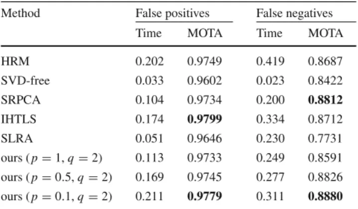
where g = ve c ( QR T) and A is a linear map. Return ˆH= QR T. Structured Rob u st PCA (SRPCA) ( A y azoglu et al. 2012 )m inˆH , E i wi σi ( ˆH) + W e ◦ E 1 + 12 W F ◦ E 2 F ✔✔ s.t. H = ˆH+ E ; ˆH, E ∈ SH . Related m ethods Iterati v e H ank el T otal Least S quares (IHTLS) ( Dicle et al. 2013 )G iv en H =[ F | g ]∈ SH , estimate ˆH=[ F + E | g + k ] by solving✗✗
min x , E , k W ◦[ E | k ] 2 F s.t. ( F + E ) x = g + k ; [ F | g ] , [ E | k ]∈ SH . Structured Lo w-Rank Approximation (SLRA) ( Mark o v sk y 2014 )m inG F ( G ) s.t. G ∈ R ( M − K ) × M has full ro w rank,✗✗
where F ( G ) := min L W ◦ ( M − L ) 2 F s.t. G H ( M ) = 0 . F o r all methods, the observ ed d ata m atrix, its Hank el v ersion, and the estimated (Hank el) structured lo w-rank approximate are d enoted by M ∈ R D × T, H = H ( M ) ∈ R M × Nand ˆH= H ( L ) ∈ R M × N, respecti v ely , unless o therwise stated3 Problem Formulation
LetM= [m0m1 . . . mT−1] ∈RD×T be a matrix contain-ing in its columns contaminated by gross but sparse noise, time varying data. The goal is to robustly learn the dynamics underlying the data, in the presence of sparse, non-Gaussian noise and missing data.
To this end, we seek to decomposeMas a superposition of two matrices:M=L+E, whereL∈RD×TandE∈RD×T, such that the Hankel matrix ofL(i.e.,H(L)∈RM×N) be of minimum rank andEbe sparse. The minimum rank ofH(L) correspond to the minimum-order LTI system that describes the data, while by imposingEto be sparse, we account for sparse, non-Gaussian noise.
A natural estimator accounting for the low-rank of the Hankel matrixH(L)and the sparsity ofEis to minimize the rank ofH(L)and the number of non-zero entries ofE, mea-sured by the0 (quasi)-norm. This is equivalent to solving
the following non-convex optimization problem.
min
L rank(H(L))+λM−L0, (8) whereλis a positive parameter. Clearly, (8) is a robust version of the Hankel structured rank minimization problem (7).
Problem (8) is intractable, as both rank and 0-norm
minimization are NP-hard (Vandenberghe and Boyd 1996; Natarajan 1995). In order to tackle this NP-hard problem, both convex and non-convex relaxations of the rank function and the0-norm are considered. To this end, we choose to
approximate the rank function and the0-norm by the
Schat-tenp- and theq-norm, respectively, and solve min L H(L) p Sp +λM−L q q, (9)
which is a convex optimization problem forp=q =1 (i.e., the Schatten 1-norm is by definition the nuclear norm) and non-convex for 0<p,q <1.
Convex approximations of the rank function and the 0-(quasi)-norm by means of the nuclear norm (i.e.,
Schat-ten 1-norm) (Fazel et al. 2001) and the1-norm (Donoho 2006) have been widely applied in several rank and spar-sity minimization problems (e.g.,Candès et al. 2011). The main advantage of this approach is that the global opti-mum of the convex problems can be found relatively easily by using off-the-shelf optimization methods such as the ADMM. However, the convexification of rank minimiza-tion problems may suffer from the following two drawbacks. First, the recoverability of the low-rank solutions via nuclear norm minimization is only guaranteed under incoherence assumptions(e.g., Candès et al. 2011). Such assumptions regarding incoherence may not be guaranteed in practical
scenarios (Dai and Li 2014). For example in the proposed model, the resulting global optimal solution of the convex instance of (9) (p,q ≥1) may be arbitrarily away from the actual solution of (8). Second, it is known that the1-norm
is a biased estimator (e.g., Zhang 2010). Since the nuclear norm (or equivalently the Schatten-1 norm) is essentially the application of the 1 norm on the singular values, it may
only find a biased solution. To alleviate the aforementioned issues of the convex instance of (9), we further consider the non-convex approximation of (8) by employing the
Schatten-pnorm andq-norm with p,q ∈ (0,1). Such non-convex functions have been shown to provide better estimation accu-racy and variable selection consistency (Wang et al. 2014b) in related approximations of0-norm regularized rank
min-imization problems (Nie et al. 2012, 2013; Papamakarios et al. 2014).
To disentangle the Schattenp- andq-norm minimization sub-problems in (9) from the matrix structure and data-fitting requirements, respectively, (9) is equivalently written as
min N,L,EN p Sp +λE q q s.t. M=L+E N=H(L) . (10)
To account also for (partially) missing observations inM, we introduce the matrixW∈RD×T which is given by
wi j =
1, if(i,j)∈,
0, otherwise, (11)
where⊂ [1,D] × [1,T]is the set containing the indices of the observed (available) entries inM. By incorporatingW inside theq-norm term in (10) as a multiplicative weight matrix forE, we arrive at the following problem.
min N,L,EN p Sp +λW◦E q q s.t. M=L+E N=H(L) . (12)
Remark Note that the choice of the Hankel map H(·) depends on the application (see Sects.2.2,5). In any case, the Hankel matrix HD,1,j,k(L)∈ R(M=D j)×(N=k) is computed according to (1); the number of blocks along the row and column dimension jandk, respectively, are set toj =r+1 andT−r, whereT is the number of observations andr >n, withndenoting the system order.
4 Algorithmic Frameworks
In this section, the proposed Alternating-Directions Method of Multipliers (ADMM)-based (Bertsekas 2014) solver is described along its scalable version.
4.1 Alternating-Direction Method-Based Algorithm The ADMM is employed to solve (12). To this end, the aug-mented Lagrangian function for (12) is defined as follows.
L(V,Y, μ) = NSp p+λW◦E q q + M−L−E,1 + N−H(L),2 +μ 2 M−L−EF2 + N−H(L)2F , (13)
whereμis a positive parameter andV:= {N∈RM×N,L∈ RD×T,E ∈ RD×T}, Y := {1 ∈ RD×T,2 ∈ RM×N} are the sets containing all the unknown variables and the Lagrange multipliers for the equality constraints in (12), respectively. Specifically, at each iteration of the proposed ADMM-based solver, (13) is minimized with respect to each variable inVin an alternating fashion and, subsequently, the Lagrange multipliers inYand the parameterμare updated. The iteration index is denoted herein by i. The notation L(N,Y[i], μ[i])is used to denote the solution stage in which all other variables butNare kept fixed, and similarly for the other unknown variables.
The solutions of minimization of (13) with respect to EandNare based on the operators and Lemmas that are introduced next. Minimizing (13) with respect to L does not admit a closed form solution due to the presence of the quadratic terms. Similarly toFazel et al.(2013), to ‘cancel out’ these terms we add a proximal term to the respective par-tial augmented Lagrangian. The additive term is based on the (semi-) norm·Q0 induced by the (semi-) inner product PTQ0P, withQ0being the positive (semi-) definite matrix
given by
Q0=LI−H∗H0, (14)
where L := min{j,k}. As shown in Sect. 2.1,√L is the upper bound of the spectral norm of the Hankel adjoint map H∗.
Thus, given the variablesV[i], the Lagrange multipliers Y[i]and the parameterμ[i]at iterationi, the updates of the proposed solver, summarized in Algorithm1, are as follows.
Update the Primal Variables E[i+1] =arg min E L( E,Y[i], μ[i]) =arg min E λμ[i]−1 W◦Eqq +1 2 E− M−L+μ[i]−11[i] 2 F (15) N[i+1]=arg min N L(N,Y[i], μ[i]) =arg min N μ[i]−1 NSpp +1 2 N− H(L)−μ[i]−12[i]2 F (16) L[i+1]=arg min L L(L,Y[i], μ[i])+μ[i] 2 L−L[i] 2 Q0 (17)
Update the Lagrange Multipliers
1[i+1] =1[i] +μ[i](M−L−E) (18)
2[i+1] =2[i] +μ[i](N−H(L)) (19) Equation (15), which offers the update forE, is solved based on thegeneralized soft thresholding operatorproposed inNie et al.(2013) and briefly described next. Consider the following problem. arg min B α Bqq+ 1 2B−Z 2 F, (20)
withB∈Rm×nandαa positive parameter. Problem (20) is separable with respect to the elements ofBand is thereby decomposed intom×nsub-problems of the form
min bi j α|bi j|q+ 1 2(bi j−zi j) 2. (21)
Let us now defineh(bi j) =α|bi j|q +12(bi j −zi j)2,c1 = (αq(1−q))2−1q andc2 = c1+αq|c1|q−1. Equation (21)
admits an analytical solution forq ∈(0,1]given by
b∗i j = ⎧ ⎪ ⎨ ⎪ ⎩ 0 if|bi j| ≤c2 arg minbi j∈{0,ρ1}h(bi j) ifbi j >c2 arg minbi j∈{0,ρ2}h(bi j) ifbi j <−c2, (22)
whereρ1andρ2are the roots ofh(bi j)=αq|bi j|q−1sgn(bi j) +bi j −zi j = 0 in [c1,zi j] and [zi j,−c1], respectively. The roots can easily be found by applying the iterative Newton–Raphson root-finding method initialized atzi j. Sim-ilarly toPapamakarios et al.(2014), we henceforth call the element-wise solver (22)generalized q-shrinkage operator
and denote it by Sαq{·}. Note that when q = 1 the afore-mentioned operator reduces to the element-wise application of the well-knownshrinkage operator(Candès et al. 2011), defined by
Sα{x} :=sgn(x)max{|x| −α,0}. (23)
We shall denote by S(α,q W){·}the operator for which α¯ = αwi j, withW∈ Rm×nknown, is used instead ofαfor the solution of each respectivebi jin (22).
The solution of (16), that is, the minimization of (13) with respect toN, is based on the following Lemma.
Algorithm 1ADMM solver for (12).
Input:Data:M∈RD×T. Weights:W∈RD×T. Parameters:{p,q, λ}. Definitions:H(·).
1: Setr= T+2
d+m+1, j=r+1,k=T−j+1,M=D j,N =k,
L=min{j,k},ρ=1.05,μmax=1010,1>0, 2>0. 2: Initialize: SetL[0] =1.1Mand1[0],2[0]to zero matrices.
Setμ[0] =L(2λM)−1. 3:whilenot convergeddo
4: E[i+1] ←Sq λμ[i]−1,W M−L[i] +μ[i]−11[i] . 5: N[i+1] ←Dp (μ[i]−1) H(L[i])−μ[i]−12[i] . 6: L[i+1] ← L+11 H∗N[i+1] +μ[i]−1 2[i] −H(L[i]) + μ[i]−11[i] +M−E[i+1] +LL[i] . 7: Update the Lagrange multipliers by (18), (19). 8: Updateμ:μ[i+1] =min(ρμ[i], μmax). 9:end while
Output:V= {N∈RM×N,L∈RD×T,E∈RD×T}.
Lemma 1 (Nie et al. 2013)The solution of the optimization problem arg min B aBSp p + 1 2B−Z 2 F, (24)
with p ∈ (0,1], is given by B = USSαp{}VST, where USVST =Zis the SVD ofZ.
We shall denote byDαp{·}the operator – henceforth called
generalized singular value p-shrinkage operator – that solves (24).
Clearly, problem (17) admits a closed-form solution. The proposed ADMM-based solver is summarized in Algorithm 1. The latter is terminated when the following conditions are met
⎧ ⎪ ⎪ ⎪ ⎪ ⎪ ⎪ ⎪ ⎪ ⎪ ⎪ ⎪ ⎪ ⎪ ⎪ ⎪ ⎪ ⎨ ⎪ ⎪ ⎪ ⎪ ⎪ ⎪ ⎪ ⎪ ⎪ ⎪ ⎪ ⎪ ⎪ ⎪ ⎪ ⎪ ⎩ max M−L[i+1] −E[i+1]F MF , N[i+1] −H(L[i+1])F MF < 1, max N[i+1] −N[i]F MF ,L[i+1] −L[i]F MF , E[i+1] −E[i]F MF < 2, ⎫ ⎪ ⎪ ⎪ ⎪ ⎪ ⎪ ⎪ ⎪ ⎪ ⎪ ⎪ ⎪ ⎪ ⎪ ⎪ ⎪ ⎬ ⎪ ⎪ ⎪ ⎪ ⎪ ⎪ ⎪ ⎪ ⎪ ⎪ ⎪ ⎪ ⎪ ⎪ ⎪ ⎪ ⎭ (25)
where1and2are small positive parameters, or a maximum
of 1000 iterations are reached.
Computational Complexity and Convergence The cost of each iteration in Algorithm1is dominated by the calculation of thegeneralized singular value p-shrinkage operator in Step 5, which involves a complexity equal to that of SVD, i.e., Omax{M2N,M N2}. Thegeneralized q-shrinkage oper-ator, utilized in Step 4, entails linear complexityO(DT).
Regarding the convergence of Algorithm 1, there is no established convergence proof of the ADMM for problems in the form of (12). Indeed, the ADMM is only known to con-verge for convex separable problems with up to two blocks of variables (e.g.,Bertsekas 2014;Candès et al. 2011). How-ever, this is not the case even in the convex instance of (12) (i.e., when p = q = 1), since the optimization problem involves more than two blocks of variables. For the multi-block separable convex problems, with three or more multi-blocks of variables, it is known that the original ADMM is not nec-essarily convergent (Chen et al. 2016). On the other hand, theoretical convergence analysis of the ADMM for non-convex problems is rather limited, making either assumptions on the iterates of the algorithm (Xu et al. 2012;Magnusson et al. 2016) or dealing with special non-convex models (Li and Pong 2015;Wang et al. 2014a, 2015), none of which is applicable for the proposed optimization problem (12). However, it is worth noting that the ADMM exhibits good numerical performance in convex problems such as non-negative matrix factorization (Sun and Févotte 2014), tensor decomposition (Liavas and Sidiropoulos 2015), matrix sep-aration (Shen et al. 2014;Papamakarios et al. 2014), matrix completion (Xu et al. 2012), motion segmentation (Li et al. 2014), to mention but a few.
To the best of our knowledge, the only work which focuses on the convergence analysis of the ADMM when applied for the optimization of piecewise linear functions such as the Schatten p-norm and theq-norm (when 0< p,q ≤ 1) is the recent preprint ofWang et al.(2016). However, since a systematic convergence analysis is out of the scope of this paper, we plan to adapt the analysis inWang et al.(2016) in order to analyze the convergence of the proposed algorithm in the future.
Even though we cannot theoretically guarantee the con-vergence of the proposed solver, the experimental results on synthetic data in Sect.6.1show that its numerical per-formance is good in practice. Specifically, the empirical convergence of the proposed solver is evidenced, where both the primal residual and the primal objective are non-increasing after the very few iterations (see Fig.2). Similar convergence behavior characterizes also the experiments on real-world data presented in Sect.6, where we have observed that even the non-convex variant with p =q =0.1 of the proposed method (12) needs no more than 180 iterations to converge in most cases.
4.2 Scalable Version of the Algorithm
To improve the scalability and reduce the computational com-plexity of the ADMM-based Algorithm1, we develop here a scalable version. Depending on the application, and more specifically, the number of inputs and/or outputs employed and the number of observations, the dimension of the
Han-Fig. 2 (Better viewed incolor). Empirical convergence analysis results for three different initializations of the proposed solver [Algorithm 1 with(p,q)=(0.5,0.5)] illustrated for the reconstruction of synthetic data corresponding to system ordern =6. The graphs illustrated are plots of the value ofathePrimal ObjectiveNSp
p+λE q q, andb
thePrimal ResidualM−L−EF of the proposed method (12),
with the iteration index. Note thatM= ˜ydenotes the given noisy data andL= ˆythe reconstruction in this experiment. The different initial-izations of the matrixLin Algorithm 1 correspond to the following scenarios: {‘multiple’:L[0] = 1.1y˜, ‘zeros’:L[0] = 0, ‘gaussian’:
L[0][t] ∼N(0,1),t=1,2, . . . ,T(mean value over 10 repetitions)},
whereTdenotes the number of observations (Color figure online) kel matrixH(L)∈RM×Ncan rise largely, which makes the
calculation of SVD prohibitive. To alleviate the aforemen-tioned computational complexity issue, we further impose thatH(L)∈RM×Nis factorized into an orthonormal matrix and a low-rank matrix asH(L)= QR, withQ ∈ RM×K, R ∈ RK×N and K M,N. In this factorization, Q ∈ RM×K is a column-orthogonal matrix satisfyingQTQ=I andR∈RK×Nis a low-rank matrix representing the embed-ding ofH(L)onto theK-dimensional subspace spanned by the columns ofQ.
Due to the unitary invariance of the Schatten p-norm, the following equality holdsQRSp = RSp. Thus, by
incorporating the factorizationH(L)=QRand adding the orthonormality constraint forQ, (12) is written as
min R,L,E,Q R p Sp +λW◦E q q s.t. ⎧ ⎨ ⎩ M=L+E, QR=H(L), QQ=I. ⎫ ⎬ ⎭ (26)
Since M K +K N M N, the number of variables has been significantly reduced. Clearly, this modification reduces the overall complexity of the method, since the SVD is now applied onM×KandK×Nmatrices as opposed to aM×N
matrix.
The ADMM is employed to solve (26). WithV:= {R∈
RK×N,L ∈ RD×T,E ∈ RD×T,Q ∈ RM×K} andY :=
{1 ∈RD×T,2 ∈RM×N}defined as the sets containing all the unknown variables and the Lagrange multipliers for the first two equality constraints in (26), respectively, the (partial) augmented Lagrangian function is defined as
Lsc(V,Y, μ) = RSp p +λW◦E q q + M−L−E,1 + QR−H(L),2 +μ 2 M−L−E2F+ QR−H(L)2F , (27)
whereμis a positive parameter. Therefore, at each iteration of the ADMM-based solver for (26), we solve
min
V L
sc(V,Y, μ)
s.t. QQ=I, (28)
with respect to each variable in V in an alternating fash-ion and, subsequently, the Lagrange multipliers inYand the parameterμare updated.
The proposed solver for (26) is summarized in Algo-rithm 2. The updates for R,L,E are similar to those employed to solve (12). The solution of (28) with respect toQis based on theProcrustes operator, which is defined asP[L] =ABT for a matrixLwith SVDL=ABT and solves the problem in the following Lemma.
Lemma 2 (Zou et al. 2006)The constrained minimization problem:
arg min B
A−B2F s.t. BTB=I (29)
has a closed-form solution given byP=P[A].
Computational Complexity and Convergence The cost of each iteration in Algorithm2 is dominated by the calcula-tion of thegeneralized singular value p-shrinkage operator
and the Procrustes operator in Step 5 and 6, respectively, which both rely on SVD, thus involving respective complex-ities of Omax{K2N,K N2}andOmax{M2K,M K2}. It is worth stressing again that choosingK M,N, which impliesM K+K N M N, leads to a significantly reduced overall complexity for Algorithm2compared to that of Algo-rithm1, which is instead dominated by a SVD on aM ×N
matrix, henceOmax{M2N,M N2}. Again, the general-ized q-shrinkage operator, utilized in Step 4, entails linear complexityO(DT).
Algorithm 2ADMM solver for (26) (scalable version).
Input:Data:M∈RD×T. Weights:W∈RD×T. Parameters:{p,q, λ}, number of componentsK. Definitions:H(·).
1: Setr= T+2
d+m+1, j=r+1,k=T−j+1,M=D j,N =k,
L=min{j,k},ρ=1.05,μmax=1010,1>0, 2>0.
2: Initialize: SetQ[0],1[0],2[0] to zero matrices and L[0] =
1.1M. Setμ[0] =L(2λM)−1. 3:whilenot convergeddo
4: E[i+1] ←Sq λμ[i]−1,W M−L[i] +μ[i]−11[i] . 5: R[i+1] ←D(pμ[i]−1) QT[i]H(L[i])−μ[i]−12[i] . 6: Q[i+1] ←P H(L[i])−μ[i]−12[i] RT[i+1] . 7: L[i+1] ← L1+1 H∗Q[i +1]R[i+1] +μ[i]−1 2[i] − H(L[i]) +μ[i]−11[i] +M−E[i+1] +LL[i] . 8: Update the Lagrange multipliers by (18), (19). 9: Updateμ:μ[i+1] =min(ρμ[i], μmax). 10:end while
Output:V= {R∈RK×N,L∈RD×T,E∈RD×T,Q∈RM×K}.
Regarding the convergence of Algorithm2which solves the scalable version of the proposed model (26), there is no yet established convergence proof of the ADMM for prob-lems in the form of (26). The discussion provided above on the convergence of Algorithm1applies to a large extent for Algorithm 2 as well. As a matter of fact, theoreti-cal analysis for the convergence of Algorithm2 becomes more challenging, compared to the case of Algorithm 1, considering that the factorizationQR=H(L)and the non-linear orthonormality constraintQQ = Iare introduced in the scalable version of the proposed model (26). It is also worth noting that problem (26) is always non-convex due to these two equality constraints, and thus the solu-tions yielded by the optimization problems (12) and (26) cannot be related. However, it has been shown inLiu and Yan(2012) that the ADMM converges to a local minimum for a problem similar to problem (26) with convex objec-tive function, i.e., p,q ≥1. To the best of our knowledge, for the case 0< p,q <1, i.e., when the Schattenp-norm and theq-norm act as non-convex approximations of the rank function and the0-(quasi) norm, respectively, there
has been no theoretical evidence for the convergence of the ADMM for the problem (26) and further investigation is needed.
Nevertheless, the ADMM has been shown to achieve good numerical performance in non-convex subspace learn-ing problems employlearn-ing a similar matrix factorization approach with one of the factors being orthonormal ( Sag-onas et al. 2014; Papamakarios et al. 2014). Also, exper-imental results on synthetic data evidence the empirical convergence of Algorithm2, which has been found to be similar to that shown for Algorithm 1 (p = q = 0.5)
in Fig. 2. Good numerical performance is also achieved by the scalable solver in the experiments presented in Sect.6.
5 Dynamic Behavior Analysis Frameworks based
on Hankel Structured Rank Minimization
In this section, we develop two frameworks for dynamic behavior analysis.5.1 Dynamic Behavior Prediction
Consider the case where continuous-time, real-valued anno-tations characterizing dynamic behavior or affect (e.g., con-flict, valence, arousal), manifested in a video sequence ofT
frames, are available for a number of consecutive framest =
0,1, . . . ,Ttr ai n−1 (training set). The goal herein is to first learn a low-order LTI system that generates the annotations as outputs Y = [y0,y1, . . . ,yTtrain−1] ∈ R
m×Ttr ai n when
visual features act as inputsU = [u0,u1, . . . ,uTtrain−1] ∈
Rd×Ttr ai n, and next use it to predict behavior measurementsytˆ
for the remaining frames of the sequencet =Ttr ai n, . . . ,T−
1 (test set), based on the respective featuresut. To this end, the following framework is proposed.
First, the proposed structured minimization problem (10) is solved, withM = Y and the Hankel mapH(·)defined as in Sect. 2.2, to estimate the system order. Second, the low-rank solutionH(L)is used to estimate the system matri-ces A,ˆ B,ˆ C,ˆ Dˆ and the initial state vectorxˆ0 by solving a
system of linear equations, following, for example,Van Over-schee and De Moor (2012). Finally, test set predictions yˆ (t =Ttr ai n, . . . ,T −1) for dynamic behavior are obtained by applying the equations of the learned state-space model (3) fort =0,1, . . . ,Ttr ai n−1, with the visual features used as inputsut.
Applications The aforementioned framework can be used for continuous prediction of any number or type of real-valued behavioral attributes manifested in a video sequence, by employing a portion of consecutive frames (even a few seconds) to learn a LTI system as described above (see Sect.6).
5.2 Dynamic Behavior Prediction with Partially Missing Outputs
Consider now the scenario in which the goal is to predict
missing(or unreliable) and not necessarily consecutive real-valued measurements of dynamic behavior or affect, viewed as missing outputsyt¯ of a low-order LTI system, directly by employing the observed visual features as inputsutand the available annotations as outputsyt, without explicitly
learn-ing the system. Herein, we approach this task as a (Hankel) structured low-rankmatrix completionproblem and address it by means of the following predictive framework that is based on the proposed model (12).
Let Y = [y0,y1, . . . ,yT−1] ∈ Rm×T and U =
[u0,u1, . . . ,yT−1] ∈ Rm×T be the matrices containing all T observations (available and missing) of inputs and outputs, respectively, and let M =
! Y U " ∈ RD×T and H(M) = HD,1,r+1,T−r ! Y U " , with D = m +d. Let also ⊂ [1,D] × [1,T]be the set containing the indices of the observed (available) entries inM. When outputs are noisy, the following property holds only approximately (Van Overschee and De Moor 2012), under the assumption of per-sistently exciting inputs.
rank(H(M))=n+rank(H(U)) . (30)
Thus, a low-rank approximation ofH(M)should be obtained to estimate the true order of the systemn.
To this end, the proposed model (12) is solved, with M defined as above and W computed according to (11). Note that this process simultaneously ‘completes’ the miss-ing observations of M, by forcing the approximation of H(M)to be low-rank, or in other words, the ‘completed’ trajectory L to follow the same linear dynamics underly-ing the observed trajectoryM. Finally, the missing outputs are recovered from the respective entries of the low-rank approximationH(L). Notably, this framework has the advan-tage that the missing observations are obtained directly by solving (12), thus avoiding the computational load asso-ciated with learning a minimum order realization of the system.
Applications The aforementioned framework can achieve prediction of missing (past or future) observations pertain-ing to dynamic human behavior or affect, with the latter used as outputs of a low-order LTI system. For instance, a computer vision problem that can be addressed by means of the proposed framework is the problem oftracklet match-ing (Ding et al. 2007a, 2008; Dicle et al. 2013), which consists of stitching trajectories of detections belonging to the same target. For this task, one needs to assess whether the joint trajectory of detectionsM = YstartY¯interYend
, where Ystart and Yend are the observed trajectories and
¯
Yinter is a zero-valued matrix corresponding to the ‘miss-ing’ intermediate trajectory, is the output of the same autonomous (output-only) LTI system that generatedYstart and Yend. This is achieved by solving (12) for Y¯inter, with M defined as above, and subsequently comparing rank(H(L))with rank(H(Ystart)) and rank(H(Yend)) (see Sect.6.4).
6 Experiments
The efficiency of the proposed structured rank minimization methods is evaluated on synthetic data corrupted by sparse, non-Gaussian noise (Sect. 6.1), as well as on real-world data with applications to: (i) conflict intensity prediction
(Sect. 6.2), (ii)valence–arousal prediction(Sect.6.3), and (iii) tracklet matching(Sect.6.4). For the case of dynamic behavior analysis experiments on real-world data, for the first two tasks, the framework described in Sect.5.1is employed, while for the last we utilize the framework described in Sect.5.2.
Aside from the proposed methods, five structured mini-mization methods are also examined, namely HRM2(Fazel et al. 2013), SVD-free (Signoretto et al. 2013), SRPCA ( Aya-zoglu et al. 2012), IHTLS (Dicle et al. 2013), and SLRA (Markovsky 2014) (see further details on these methods in Table1). For all experiments presented in our paper, a grid search is employed to tune the parameterλof the proposed methods or any other parameters of the compared methods that need tuning. Tuning is performed by following an out-of-sample evaluation, that is, the last portion of the training frames is withheld for validation and the best-performing model is used for testing. Specifically, the last 2r training observations, withrdefined in Sect.3, are kept out for vali-dation in all our experiments.
6.1 Experiment on Synthetic Data
In the experiments presented in this section, the efficiency of the proposed method (12) is evaluated on synthetic data cor-rupted with sparse, non-Gaussian noise. In order to generate Hankel matrices of given rankn, we follow the methodology proposed inPark et al.(1999), that is,T outputsy(t)of an autonomous stable LTI system of ordern are generated by applying the following formula
y(t)= n # k=1
ztk, t =1,2, . . . ,T, (31)
where zk appear in pairs of conjugate numbers so that the observationsy(t)are real numbers. It follows naturally that a M ×N Hankel matrix Y = H(y) = H1,1,M,N(y)with yderived according to (31) has rank equal ton (Park et al. 1999). Subsequently, sparse, non-Gaussian noiseη∈R1×T is added to the original signaly, with the non-zero entries following the Bernoulli model with probabilityρ =0.2, as inCandès et al.(2011). The final corrupted signal is formed asy˜ =y+η, with the corresponding noisy Hankel matrix
˜
Y=H(y)˜ being full-rank.
In what follows, the efficiency of various structured rank minimization methods in reconstructing the noiseless sys-tem outputs y(t),t = 1,2, . . . ,T, by finding a low-rank approximationYˆ =H(y)ˆ given the noisy Hankel matrixY˜, is experimentally assessed in various scenarios.
The reconstruction error, for both the noiseless observa-tions y and the noise η, is measured in terms of relative reconstruction error as follows.
err(s,ˆs)=s− ˆs
s , (32)
withsdenoting the original signal andsˆdenoting the esti-mated signal by the algorithm.
Experiment with Varying System Orders Herein, experi-ments are conducted for various orders of the LTI system generating the ‘clean’ data, as described above. Specifi-cally, the system ordern is varied in{6,12,18}. For each value ofn the experiment is repeated 10 times, that is, for 10 different output trajectories y ∈ R1×T computed by randomly selecting the complex coefficients in (31). For the proposed model, Algorithm 1 is used and the follow-ing combinations are examined for the p and q values corresponding to the Schatten p- and q-norm, respec-tively: (p,q) ∈ {(1,1), (0.9,0.9), (0.5,0.5), (0.1,0.1)}. The methods HRM, SVD-free, SRPCA, IHTLS, and SLRA (listed in Table1) are also evaluated for comparison. For each method, results are reported in terms of minimum reconstruc-tion error err(y,y)ˆ computed according to (32). Performance is also evaluated in terms of reconstruction error for the noise signal err(η,ηˆ) and the Pearson Correlation Coeffi-cient (COR) measured between the noiseless observationsy and the reconstructed outputsyˆ.
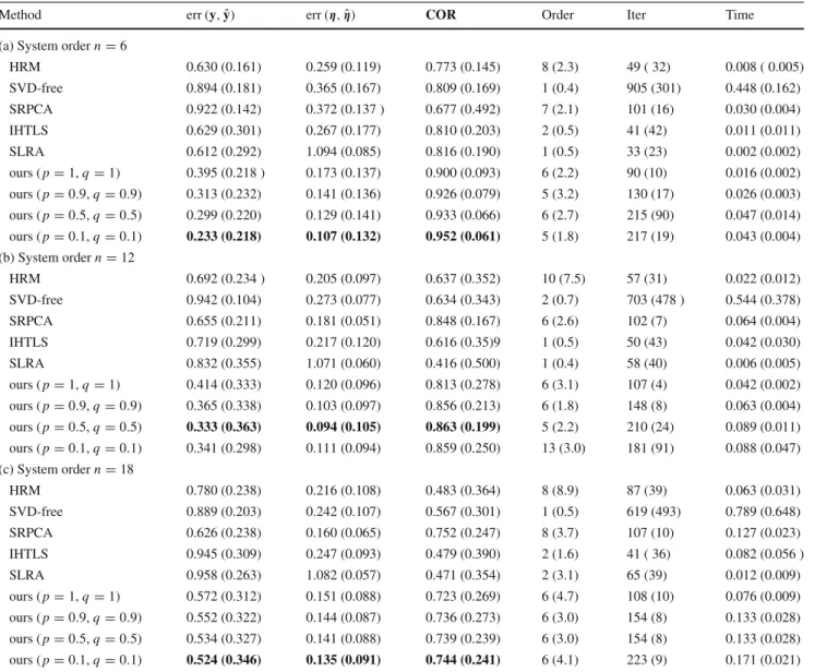
Table 2a–c contain the results obtained by the various methods for system order n = 6, n = 12 andn = 18, respectively. Specifically, mean and standard deviation val-ues of the reconstruction errors err(y,y)ˆ and err(η,ηˆ)and the COR values computed over the 10 trials of each experiment are reported. The mean values of the estimated system order (rank ofYˆ =H(yˆ)), number of iterations and execution time are also reported.
Firstly, we observe that the non-convex instances of the proposed method, i.e., whenp,q<1, consistently account for the most accurate reconstruction of both the clean sig-nal, in terms of both reconstruction error and correlation, as well as the recovery of the sparse noise. In most cases, the performance is improved when smaller values for p
andq are chosen for the proposed model. Secondly, all the compared methods (HRM, SVD-free, SRPCA, IHTLS and SLRA) achieve much lower performance in terms of all the three metrics employed. Furthermore, it is worth noting that, in the scenarios corresponding to ordersn=12 andn=18,
SRPCA recovers the noise more accurately than the HRM, SVD-free, IHTLS and SLRA. This is expected since the for-mer is the only method amongst the compared ones that is robust to sparse, non-Gaussian noise. It is also worth men-tioning that the system order pertaining to the recovered observations varies significantly amongst different methods. Amongst the different instances of the proposed method, this variation is much smaller, with the only exception being the result obtained by our method with(p,q)=(0.1,0.1) for the casen = 12. Regarding the number of iterations, which varies largely across methods, we observe that the non-convex instances of the proposed method require a larger amount of iterations to converge, as compared to the con-vex instance (p = q = 1). However, even in the scenario of order n = 18, the best-performing instance of the pro-posed method (p=q =0.1) needs 223 iterations in average to converge. Finally, the execution times corresponding to the best-performing, non-convex instances of the proposed method in all three experiments are comparable to those accounted for by even convex compared methods, such as SRPCA.
Empirical Convergence Analysis In this experiment, the convergence of the proposed method is assessed by employ-ing various types of initialization. To this end, we employ synthetic data corrupted with sparse, non-Gaussian noise, generated similarly to the previous experiment. We clar-ify here that the only variable that needs to be initialized in Algorithm 1, except for the Lagrange multipliers, is the matrix L. All other variables are calculated in the 1st iteration of the ADMM loop according to the respective updates.
The proposed solver is executed using the following three types of initialization, namely, ‘original signal’:L[0] =1.1y˜, ‘zeros’: L[0] = 0, ‘gaussian’: L[0][t] ∼ N(0,1), t =
1,2, . . . ,T, wherey˜ denote the noisy system outputs con-structed as in the previous experiments andN(0,1)denotes the normal distribution. For each type of initialization, the values of the primal objective (NSp
p +λE
q q) and the primal residual (M −L −EF ) of the proposed model (12) are plotted as a function of the iteration index in Fig. 2. Here M = ˜y denotes the given noisy data and L = ˆy the reconstruction. These plots enable us to demonstrate the convergence of the proposed solver. Note that for the last initialization scenario, the experiment is repeated 10 times. and the average convergence curve is plot-ted.
By inspecting both graphs, it is evident that all three ini-tializations lead to similar convergence behavior in the sense that both the primal objective and the primal residual are non-increasing after the first few iterations. However, by ini-tializing the algorithm using the scaled version of the original signal (L[0] =1.1y˜) the primal objective attains smaller
val-Table 2 Recovery results obtained by the proposed method and the compared methods corresponding to system order (a)n=6, (b)n=12 and (c)n=18
Method err(y,yˆ) err(η,η)ˆ COR Order Iter Time
(a) System ordern=6
HRM 0.630 (0.161) 0.259 (0.119) 0.773 (0.145) 8 (2.3) 49 ( 32) 0.008 ( 0.005) SVD-free 0.894 (0.181) 0.365 (0.167) 0.809 (0.169) 1 (0.4) 905 (301) 0.448 (0.162) SRPCA 0.922 (0.142) 0.372 (0.137 ) 0.677 (0.492) 7 (2.1) 101 (16) 0.030 (0.004) IHTLS 0.629 (0.301) 0.267 (0.177) 0.810 (0.203) 2 (0.5) 41 (42) 0.011 (0.011) SLRA 0.612 (0.292) 1.094 (0.085) 0.816 (0.190) 1 (0.5) 33 (23) 0.002 (0.002) ours (p=1,q=1) 0.395 (0.218 ) 0.173 (0.137) 0.900 (0.093) 6 (2.2) 90 (10) 0.016 (0.002) ours (p=0.9,q=0.9) 0.313 (0.232) 0.141 (0.136) 0.926 (0.079) 5 (3.2) 130 (17) 0.026 (0.003) ours (p=0.5,q=0.5) 0.299 (0.220) 0.129 (0.141) 0.933 (0.066) 6 (2.7) 215 (90) 0.047 (0.014) ours (p=0.1,q=0.1) 0.233 (0.218) 0.107 (0.132) 0.952 (0.061) 5 (1.8) 217 (19) 0.043 (0.004) (b) System ordern=12 HRM 0.692 (0.234 ) 0.205 (0.097) 0.637 (0.352) 10 (7.5) 57 (31) 0.022 (0.012) SVD-free 0.942 (0.104) 0.273 (0.077) 0.634 (0.343) 2 (0.7) 703 (478 ) 0.544 (0.378) SRPCA 0.655 (0.211) 0.181 (0.051) 0.848 (0.167) 6 (2.6) 102 (7) 0.064 (0.004) IHTLS 0.719 (0.299) 0.217 (0.120) 0.616 (0.35)9 1 (0.5) 50 (43) 0.042 (0.030) SLRA 0.832 (0.355) 1.071 (0.060) 0.416 (0.500) 1 (0.4) 58 (40) 0.006 (0.005) ours (p=1,q=1) 0.414 (0.333) 0.120 (0.096) 0.813 (0.278) 6 (3.1) 107 (4) 0.042 (0.002) ours (p=0.9,q=0.9) 0.365 (0.338) 0.103 (0.097) 0.856 (0.213) 6 (1.8) 148 (8) 0.063 (0.004) ours (p=0.5,q=0.5) 0.333 (0.363) 0.094 (0.105) 0.863 (0.199) 5 (2.2) 210 (24) 0.089 (0.011) ours (p=0.1,q=0.1) 0.341 (0.298) 0.111 (0.094) 0.859 (0.250) 13 (3.0) 181 (91) 0.088 (0.047) (c) System ordern=18 HRM 0.780 (0.238) 0.216 (0.108) 0.483 (0.364) 8 (8.9) 87 (39) 0.063 (0.031) SVD-free 0.889 (0.203) 0.242 (0.107) 0.567 (0.301) 1 (0.5) 619 (493) 0.789 (0.648) SRPCA 0.626 (0.238) 0.160 (0.065) 0.752 (0.247) 8 (3.7) 107 (10) 0.127 (0.023) IHTLS 0.945 (0.309) 0.247 (0.093) 0.479 (0.390) 2 (1.6) 41 ( 36) 0.082 (0.056 ) SLRA 0.958 (0.263) 1.082 (0.057) 0.471 (0.354) 2 (3.1) 65 (39) 0.012 (0.009) ours (p=1,q=1) 0.572 (0.312) 0.151 (0.088) 0.723 (0.269) 6 (4.7) 108 (10) 0.076 (0.009) ours (p=0.9,q=0.9) 0.552 (0.322) 0.144 (0.087) 0.736 (0.273) 6 (3.0) 154 (8) 0.133 (0.028) ours (p=0.5,q=0.5) 0.534 (0.327) 0.141 (0.088) 0.739 (0.239) 6 (3.0) 154 (8) 0.133 (0.028) ours (p=0.1,q=0.1) 0.524 (0.346) 0.135 (0.091) 0.744 (0.241) 6 (4.1) 223 (9) 0.171 (0.021) The bold values indicate the best performances in terms of each evaluation metric
Results are reported in terms of mean values over 10 repetitions of the experiment, while standard deviation values are reported inside parentheses
ues than the other two types of initialization. This justifies our choice of initialization asL[0] = 1.1y˜ in the proposed algorithms.
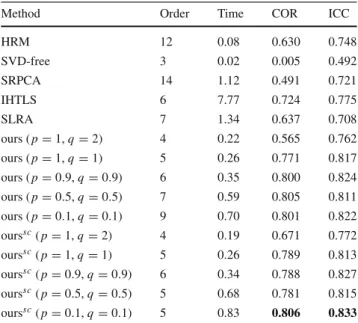
6.2 Conflict Intensity Prediction
In this section, we address the problem of continuous con-flictintensity prediction based on the visual modality only. Conflict is usually defined as disagreement of high inten-sity or escalation, in which at least one of the involved interlocutors feels emotionally offended (Bousmalis et al. 2009). Hence, various challenges are posed to machine anal-ysis of conflict in real-world competitive conversations, since simultaneous processing of the data streams from all
inter-actants is required. Furthermore, when the visual modality is also considered, feature extraction has to cope with vari-ous types of visual noise, such as extreme head pose values and abrupt body movements, which renders computer vision pre-processing (e.g., tracking, alignment) rather difficult.
Automated approaches to conflict analysis include just a few works, which are based on audio features only (Kim et al. 2012a,b). However, visual features can help discover facial behavioral cues that are intrinsically correlated with conflict, such as smiling, blinking, head nodding, flouncing and frowning. The only audio-visual approach to conflict detection that we are aware of is Panagakis et al. (2016), where robust, multi-modal fusion of audio-visual cues is uti-lized. However, all works mentioned above address conflict