Computation of the stochastic basin of attraction by rigorous
construction of a Lyapunov function
Article (Accepted Version)
http://sro.sussex.ac.uk
Bjoernsson, Hjortur, Hafstein, Sigurdur, Giesl, Peter, Scalas, Enrico and Gudmundsson, Skuli
(2019) Computation of the stochastic basin of attraction by rigorous construction of a Lyapunov
function. Discrete and Continuous Dynamical Systems - Series B, 24 (8). pp. 4247-4269. ISSN
1531-3492
This version is available from Sussex Research Online: http://sro.sussex.ac.uk/id/eprint/80036/
This document is made available in accordance with publisher policies and may differ from the
published version or from the version of record. If you wish to cite this item you are advised to
consult the publisher’s version. Please see the URL above for details on accessing the published
version.
Copyright and reuse:
Sussex Research Online is a digital repository of the research output of the University.
Copyright and all moral rights to the version of the paper presented here belong to the individual
author(s) and/or other copyright owners. To the extent reasonable and practicable, the material
made available in SRO has been checked for eligibility before being made available.
Copies of full text items generally can be reproduced, displayed or performed and given to third
parties in any format or medium for personal research or study, educational, or not-for-profit
purposes without prior permission or charge, provided that the authors, title and full bibliographic
details are credited, a hyperlink and/or URL is given for the original metadata page and the
content is not changed in any way.
AIMS’ Journals
VolumeX, Number0X, XX200X pp.X–XX
COMPUTATION OF THE STOCHASTIC BASIN OF ATTRACTION BY RIGOROUS CONSTRUCTION OF A
LYAPUNOV FUNCTION
Hj¨ortur Bj¨ornsson, Sigurdur Hafstein Faculty of Physical Sciences
University of Iceland 107 Reykjavik, Iceland Peter Giesl, Enrico Scalas
Department of Mathematics University of Sussex Falmer BN1 9QH, United Kingdom
Skuli Gudmundsson Svensk Exportkredit Klarabergsviadukten 61-63 111 64 Stockholm, Sweden
Abstract. Theγ-basin of attraction of the zero solution of a nonlinear sto-chastic differential equation can be determined through a pair of a local and a non-local Lyapunov function. In this paper, we construct a non-local Lya-punov function by solving a second-order PDE using meshless collocation. We provide a-posteriori error estimates which guarantee that the constructed func-tion is indeed a non-local Lyapunov funcfunc-tion. Combining this method with the computation of a local Lyapunov function for the linearisation around an equi-librium of the stochastic differential equation in question, a problem which is much more manageable than computing a Lyapunov function in a large area containing the equilibrium, we provide a rigorous estimate of the stochastic
γ-basin of attraction of the equilibrium.
1. Introduction. In deterministic dynamical systems given by autonomous or-dinary differential equations (ODE), the basin of attraction of an asymptotically stable equilibrium is the set of all initial conditions, such that the corresponding solutions converge to the equilibrium as time tends to infinity. When considering a stochastic differential equation (SDE), this notion can be replaced by theγ-basin of attraction, i.e. the set of all initial conditions, such that sample paths will converge to the equilibrium as time tends to infinity with probability at leastγ. This concept will be defined in Section 2, Definition 2.2.
It turns out that the γ-basin of attraction can be determined using Lyapunov functions. In [8], a combination of a local and a non-local Lyapunov function was
2010Mathematics Subject Classification. Primary: 37B25, 65P40, 93E03, 93E15, 93D30; Sec-ondary: 60H35, 65C30.
Key words and phrases. Nonlinear stochastic differential equation, Lyapunov function, Radial basis function, Basin of attraction .
The research for this paper was supported by the Icelandic Research Fund (Rann´ıs) in the project ‘Lyapunov Methods and Stochastic Stability’ (152429-051), which is gratefully acknowledged.
used to determine a subset of the γ-basin of attraction. A Lyapunov function
V:Rd →R for a SDE satisfies LV(x)≤0, whereL is a second-order differential
operator, which arises from the SDE. A local Lyapunov function is only defined in a small neighborhood of the equilibrium and can often be determined by linearisation. A non-local Lyapunov function, however, is defined on a supersetU ⊂e Rd of theγ
-basin of attraction apart from a small neighborhood, where the negativity condition is not necessarily satisfied. Local Lyapunov functions will be defined in Section 2, Definition 2.3, and non-local ones in Section 2, Definition 2.4.
In this paper, we present a constructive method to compute a non-local Lyapunov function for a general SDE. In particular, we use meshless collocation to solve a PDE boundary value problem of the form LV(x) = ˜ν <0 for all x∈Ue and with fixed
boundary values for V(x) at all x∈ ∂Ue. After choosing a kernel, in particular a
Radial Basis Function, as well as collocation points inUe and∂Ue, the approximate
solutionvto the problem is determined by using a certain ansatz and by computing coefficients by solving a linear equation.
To ensure that the approximationvis itself a valid Lyapunov function, we provide rigorous a-posteriori estimates on Lv(x). This is achieved by evaluatingLv(x) at allxin a test grid and using Taylor-type estimates for the points in between. These make use of the specific ansatz and corresponding estimates. The method is applied to two examples in one and two dimensions, respectively.
The outline of the paper is as follows: In Section2we recall the definition of the
γ-basin of attraction and its determination using a pair of a local and a non-local Lyapunov function. In Section 3 we discuss meshless collocation for general PDE boundary value problems and in particular for the PDE related to the SDE under study. Moreover, we present a-posteriori error estimates based on first and second derivatives ofLv. Section4applies these results to the construction of a non-local Lyapunov function. Finally, we apply the method to two examples in Section 5. The appendix contains explicit formulas for the ansatz using meshless collocation, as well as tables for the estimates.
Note on notations:
If not specified, we use the Euclidean norm of a vectorx∈Rd, i.e. kxk:=kxk2.
We denote the closed-neighborhood with respect to the k · k1norm of a compact
setK⊂Rd by K,k·k1 ={x∈R d : dist k·k1 (x, K)≤}, where dist k·k1
(x, K) = miny∈Kkx−yk1. We sometimes denote the i-th component of
a vectorx−yby (x−y)i to shorten formulas.
2. Stochastic basin of attraction and Lyapunov functions. In this section we introduce the type of SDE that we study as well as the stochastic basin of attraction of the zero (trivial) solution. We also recall the definition of (stochastic) Lyapunov functions; in particular, we will consider an appropriate combination of a local and a non-local Lyapunov function to determine the stochastic basin of attraction.
We study the stability of the trivial solution of the SDE of Itˆo type
dX(t) = f(X(t))dt+g(X(t))dW(t), (2.1) where W(t) is a Q-dimensional Wiener process. The functions f : Rd →Rd and
g : Rd →
i.e. there exists aK >0 such that
kf(x)−f(y)k+kg(x)−g(y)k ≤Kkx−yk for allx,y∈ O.
Moreover, we assume thatf(0) =0andg(0) = 0, so thatX(t) =0is a solution of (2.1) for allt≥0.
Since we are interested in local stability, i.e.γ-basins of attraction withinO, we can extend f and g to Lipschitz continuous functions onRd and consider strong
solutions to (2.1) on [0,∞). This simplifies technical matters considerably, cf. [8,
§2].
For the SDE (2.1) the associatedgenerator is given by
LV(x) :=∇V(x)·f(x) +1 2 d X i,j=1 g(x)g(x)>ij ∂ 2V ∂xi∂xj (x), (2.2) forV :U →RwithU ⊂Rd.
Remark 2.1. If the matrixg(x)g(x)>is positive definite for allx∈ U in a compact setU ⊂Rd, then the second-order linear differential operatorLis strictly elliptic in U. In this (non-degenerate) case, results about the existence of classical solutions are available, however, in this paper we will discuss the general case and make no requirement on the positive definiteness of the matrix.
Let us now define the γ-basin of attraction which describes the set of initial conditions so that sample paths converge to the origin with probability at leastγ, see [8, Definition 2.4].
Definition 2.2 (γ-basin of attraction (γ-BOA)).
Consider the system (2.1) and let0< γ≤1. We refer to the set
n x∈Rd : P n lim t→∞kX x(t)k= 0o≥γo (γ-BOA)
as the γ-basin of attraction or shortγ-BOA of the origin. Here,Xx(t)denotes the
unique strong solution (stochastic process) of the SDE with initial condition x.
In the following definition [8, Definition 2.5], we introduce a local Lyapunov func-tion in the set N (see also [8, Theorem 2.7]). A local Lyapunov function U is a positive definite function such thatLU is negative definite in a (small) neighbour-hood N of 0. This is most conveniently defined using so-called K∞ functions; a
functionµ:R+ →R+is said to be of classK∞if it is continuous, strictly increasing,
µ(0) = 0, and limx→∞µ(x) =∞.
Definition 2.3(Local Lyapunov function). Consider the system (2.1). A function
U ∈ C(N)∩C2(N \ {0}), where 0 ∈ N ⊂ Rd is a domain, is called a (local)
Lyapunov function for the system (2.1), if there are functions µ1, µ2, µ3 ∈ K∞,
such that U fulfills the properties:
(i) µ1(kxk)≤U(x)≤µ2(kxk)for allx∈ N
(ii) LU(x)≤ −µ3(kxk)for allx∈ N \ {0}
Let Umax>0 be such thatU−1([0, Umax]) is a compact subset ofN.
Next we introduce a non-local Lyapunov function in the setU as in [8, Definition 2.9, (2a)]; note that we have replaced 0 by b and 1 by a. A non-local Lyapunov function satisfiesLV <0 in a large setU, not including a small neighborhoodBof the equilibrium.
Definition 2.4(Non-local Lyapunov function). LetA,B ⊂Rd,B ⊂ A◦, be simply
connected compact neighbourhoods of the origin with C2 boundaries and set U :=
A \ B◦. A function V ∈C2(U)for the system (2.1)such that
(1) b≤V(x)≤afor all x∈ U,V−1(b) =∂B,V−1(a) =∂Awith b < a, and
(2) LV(x)<0 for allx∈ U,
is called a non-local Lyapunov functionfor the system (2.1). We refer to∂Aas the outer boundary ofU and∂B as the inner boundary of U.
The following result from [8, Theorem 2.11] shows how a local and a non-local Lyapunov function provide information about the γ-BOA. For an illustration of the various sets, see [8, Figure 1]. The proof uses the non-local Lyapunov function to estimate the probability that solutions starting in U leave the set through the boundary∂B, and then the local Lyapunov function estimates the probability that they converge to the origin once they are inB. The combined probability can be bounded byγ.
Theorem 2.5. Consider the system (2.1)and assume there exists a local Lyapunov function U :N →R+ as in Definition 2.3with the constant Umax>0 and a
non-local Lyapunov function V : U → R+ as in Definition 2.4. Let 0 < β < 1 and b < λ < α < a and the setB from Definition2.4 be such that
U−1(Umax)⊂V−1([b, λ]) and ∂B=V−1(b)⊂U−1([0, β Umax]).
Then the setV−1([b, α])∪ B is a subset of the γ-BOA of the origin, where γ:= (a−α)(1−β)
a−b−β(a−λ). (2.3) Note that the bound (2.3) has a different formula than in [8, Theorem 2.11], because here∂B=V−1(b) and∂A=V−1(a) withb andanot necessarily equal to 0 and 1, respectively. Thus our formula is the formula from [8, Theorem 2.11] with
γ replaced by (γ−b)/(a−b) andαreplaced by (α−b)/(a−b).
In this paper, we focus on a general method to compute non-local Lyapunov functions. Local Lyapunov functions can often be found directly in specific exam-ples: for example, if the noise is small and the origin is an asymptotically stable equilibrium of the corresponding deterministic system with no noise, then the de-terministic Lyapunov function can serve as a local Lyapunov function. Another way to construct a local Lyapunov function is similar to the construction of local Lyapunov functions for deterministic systems: by linearising the system around the origin and constructing a Lyapunov function for the linearised system, which is a local Lyapunov function for the nonlinear system, see [1].
For the examples in this paper, we are able to construct local Lyapunov functions with one of these two approaches. For a more general discussion on the construction of Lyapunov functions for linear systems see also [9].
3. Meshless Collocation. In this section we will recall meshless collocation and its use to approximate solutions of boundary value problems for general linear PDEs of the form
LV(x) = r(x) forx∈Ω,
V(x) = c(x) forx∈∂Ω, (3.1)
where L is a linear differential operator and Ω is a bounded domain in Rd with
of an interpolation problem, which minimises the norm in a Reproducing Kernel Hilbert Space (RKHS), in our case a Sobolev space. The interpolation problem will ensure thatv satisfies the PDE and the boundary values (3.1) at given collocation points.
If the PDE boundary value problem has a solutionV, thenvapproximatesV and we have error estimates ofkV(x)−v(x)kL∞(∂Ω) as well askLV(x)−Lv(x)kL∞(Ω).
The error estimates involve the fill distance of the collocation points, measuring how dense they are in Ω and ∂Ω, respectively. Unfortunately, these estimates also involve unknown quantities, such as the norm of V. Thus, these error estimates ensure that by adding more and more collocation points the error converges to zero, but they do not provide explicit, computable bounds on the error.
We can, however, compute explicit a-posteriori bounds on the errors kV(x)− v(x)kL∞(∂Ω)as well askLV(x)−Lv(x)kL∞(Ω)by first computing|LV(x)−Lv(x)|
for a finite, but large set of pointsY ⊂Ω. Taylor’s theorem and estimates on the first and second derivatives by using the explicit form ofv provide us with explicit bounds on these errors as shown in Section3.2.
3.1. Meshless collocation: PDE boundary value problems. Meshless collo-cation, in particular by Radial Basis Functions, is a powerful method to solve linear PDEs [11, 2, 12]. For a general introduction to meshless collocation and RKHS, see [14]. Meshless collocation has been applied to the computation of Lyapunov functions in deterministic systems [4,7]. For an overview of this and other methods to compute Lyapunov functions, see the review [5].
In this section, we will outline the method, apply it to our particular case, and recall known results, in particular error estimates from [4].
We consider a general linear operatorLof ordermgiven by
LV(x) = X
|α|≤m
cα(x)∂αV(x). (3.2)
In our case,m= 2 and the operator is given by
Lv(x) = 1 2 d X i,j=1 mij(x) ∂2 ∂xi∂xj v(x) + d X i=1 fi(x) ∂ ∂xi v(x), (3.3)
where (mij(x))i,j=1,...,d=g(x)g(x)>, i.e. mij(x) =P Q
q=1giq(x)gjq(x). We denote
theq-th column ofgbygq.
Hence, our operator is of the form (3.2) with cei(x) = fi(x) and cei+ej(x) =
1
2mij(x). A singular point of Lis a point xwithcα(x) = 0 for all |α| ≤2, see [4,
Definition 3.2].
Let Ω⊂Rd be a bounded domain with smooth boundary Γ :=∂Ω. Our goal is
to (approximately) solve the boundary value problem with a PDE given by:
Lv(x) = r(x) forx∈Ω,
v(x) = c(x) forx∈Γ. (3.4)
Our approximation will be a function in a RKHS, which is a Hilbert spaceH of functions Ω→Rwith inner product h·,·iH, and a kernel Φ : Ω×Ω→Rsuch that
1. Φ(·,x)∈H for allx∈Ω,
2. g(x) =hg,Φ(·,x)iH for allx∈Ω andg∈H.
In our case, we choose the radially symmetric kernel Φ(x,y) =ψ(kx−yk), where
bd
2c+k+ 1, the parameterk∈Nis a smoothness index and the function Φ(x,y) is
a C2k function inxfor fixedy, and the RKHS with this kernel is norm-equivalent
to the Sobolev spaceWτ
2 withτ =k+
d+1 2 .
Given sets of pairwise distinct points X1 = {x1, . . . ,xN} ⊂ Ω ⊂ Rd, none of
which is a singular point of L, and pairwise distinct pointsX2 ={ξ1, . . . ,ξM} ⊂
Γ =∂Ω, we seek to find the (unique) solutionvto the interpolation problem
Lv(xi) = r(xi) for all i= 1, . . . , N, v(ξi) = c(ξi) for alli= 1, . . . , M,
which minimises the norm of the RKHS. It turns out that the solution is given by
v(x) = N X k=1 αk(δxk◦L) yψ(kx−yk) + M X k=1 αN+k(δξk◦L0)yψ(kx−yk), (3.5) whereL0= id,δ
yv(x) =v(y), the superscriptydenotes that the operator is applied
with respect to the variabley, and the coefficientsαk are computed by solving the
linear system Aα=β, where βk = r(xk) fork = 1, . . . , N andβN+k =c(ξk) for k = 1, . . . , M. A = (akl) is a symmetric (N +M)×(N +M) matrix given by A= B C C> D withB∈RN×N,C∈ RN×M,D∈RM×M, where fork, l= 1, . . . , N : bkl= (δxk◦L) x(δx l◦L) yψ(kx−yk), fork= 1, . . . , N, l= 1, . . . , M: ckl= (δxk◦L) x(δ ξl◦L0)yψ(kx−yk) = (δxk◦L) xψ( kx−ξlk), fork, l= 1, . . . , M : dkl= (δξk◦L0)x(δξl◦L0)yψ(kx−yk) =ψ(kξk−ξlk).
Explicit formulas forv andLv are given in the AppendixA.
If the PDE has a solution V, then error estimates imply that the function v is an approximation toV as stated in Theorem3.1below. Note that the mesh norms measure how dense the points in X1 and X2 are in the domain and boundary,
respectively. The following is [4, Corollary 3.12] adapted to our linear operator.
Theorem 3.1. Let k > 3/2, if d is odd, and k > 2, if d is even. Let fi, mij ∈ Wk−1+b
d+1 2 c
∞ (Ω) and let the solution V of (3.4)satisfy V ∈Wk+(d+1)/2(Ω). Then the approximationv as above, for sufficiently small mesh norms, satisfies
kLV −LvkL∞(Ω)≤Ch k−3/2 X1,Ω kVkW2k+(d+1)/2(Ω), (3.6) kV −vkL∞(∂Ω)≤Ch k+1/2 X2,∂ΩkVkW2k+(d+1)/2(Ω), (3.7)
wherehX1,Ω= supx∈Ωminxj∈X1kx−xjkand the constanthX2,∂Ωis the mesh norm
3.2. A-posteriori error estimates. Note that, unless L is non-degenerate, we have no results on the existence of classical solutions and thus we cannot use The-orem3.1. Even in that case, the error estimates in Theorem3.1contain quantities that are not known explicitly, such askVkWk+(d+1)/2
2 (Ω)
.
Hence, in this section we derive estimates that only contain explicitly computable constants. They do not require us to prove the existence of a solution, but are a verification that the computed function satisfies an inequality at all points. The main idea is to evaluate the function at many points on a test grid and then use a Taylor-type argument in between. As we have an explicit formula for the approx-imation, we can derive explicit bounds on the derivatives. As these are multiplied by the mesh norm of the test grid, which can be made arbitrarily small, we can make the estimate as accurate as necessary.
Let us first present the Taylor-type estimates for a general function u, which later will be either the approximationv or Lv. These theorems, as well as a more detailed discussion of a suitable choice of the test grid are taken from [10], see also [6].
As test grids, we will use the following:
Definition 3.2. Define the following grids in Rd with h >0 :
• Sh=hZd
• Ch=Sh∪ h21+Sh
, where1= (1, . . . ,1)∈Rd
The following theorem is based on the mean-value theorem and uses the specific structure of the grid pointsSh.
Theorem 3.3 (First derivative). Let u∈C1(
Rd,R) and let K ⊂Rd be compact.
Fix h >0 and letY :=Ch∩Kh d/4,k·k1.
Define eh= d 4z∈Kmaxh d/4,k·k1 max l∈{1,...,d} ∂u ∂xl (z) h.
Then we have for all x∈K that
min
y∈Y u(y)−eh≤u(x)≤maxy∈Y u(y) +eh.
Proof. Letx∈K. Then there is ay∈Ch withkx−yk1≤ d4h, see [10, Theorem
5.5], and thusy∈Y. The mean value theorem shows that there is aθ∈[0,1] such that |u(x)−u(y)| = |∇u(θx+ (1−θ)y)·(x−y)| ≤ k∇u(θx+ (1−θ)y)k∞kx−yk1 ≤ max l∈{1,...,d} ∂u ∂xl (θx+ (1−θ)y) d 4h . Note thatθx+ (1−θ)y∈Kh d/4,k·k1, since
kθx+ (1−θ)y−xk1= (1−θ)ky−xk1≤ d
4h. This shows the statement.
The next theorem relies on a triangulation of the phase space with vertices inSh, Ch, respectively. Using Taylor’s theorem in each simplex, we can derive the
esti-mates below. Note that, as discussed in [10], depending on odd or even dimension, we use eitherSh orCh to obtain an estimate with as few points as possible.
Theorem 3.4 (Second derivative). Letu∈C2(Rd,R)and let K⊂Rd be compact. Fix h >0. Ifd >1 define eh= d2 4 z∈Kmaxd h,k·k1 max l,p∈{1,...,d} ∂2u ∂xp∂xl (z) h2. • If dis even, then letY :=Sh∩Kd h,k·k1.
• If d≥3 is odd, then let Y :=Ch∩K(d−1)h,k·k1.
In the cased= 1 letY :=Ch∩Kh/2,k·k1 and define
eh=
1
4z∈Kmaxh/2,k·k1
|u00(z)|h2.
In all cases we then have for allx∈K
min
y∈Yu(y)−eh ≤ u(x) ≤ maxy∈Y u(y) +eh.
Proof. We consider the case wheredis even. Letx∈K. Then there is a simplexS
with vertices{x0,x1, . . . ,xd} ⊂Sh, such thatx=P d
i=0λixi∈S, whereP d i=0λi=
1 and 0≤λi ≤1. Since maxy,z∈Sky−zk1 =dh, we haveS ⊂Kd h,k·k1 and thus
{x0,x1, . . . ,xd} ⊂Y.
Now we use the following result from [10, Proposition 5.2]: Denote by h∗ := maxj=0,...,dkx0−xjk1the maximal distance from any vertex to the fixed vertexx0.
Forw∈C2(Rd,R) we have for all 0≤λi≤1 withP d i=0λi= 1 that w d X i=0 λixi ! − d X i=0 λiw(xi) ≤ max z∈S l,p∈{max1,...,d} ∂2w(z) ∂xp∂xl (h∗)2. (3.8) In our case, we can choose the vertexx0 such thath∗=d2h. Asx∈S there are
0≤λi≤1 withP d i=0λi= 1 such thatx=P d i=0λixi. Hence, by (3.8) u(x)− d X i=0 λiu(xi) ≤ max z∈Kd h,k·k1 max l,p∈{1,...,d} ∂2u(z) ∂xp∂xl d2 4 h 2 and then u(x)≤max y∈Y u(y) d X i=0 λi | {z } =1 + max z∈Kd h,k·k1 max l,p∈{1,...,d} ∂2u(z) ∂xp∂xl d2 4 h 2
and similarly for the other inequality.
The result for odd dimensions follows in a similar way, noting that we choose a simplexS with vertices{x0,x1, . . . ,xd} ⊂Ch. Since maxy,z∈Sky−zk1= (d−1)h
ford≥2 and h2 ford= 1, and for a simplex with vertices inChwe can choose the
vertex x0 such thath∗ := maxj=0,...,dkx0−xjk1 = d2h, see [10, Theorem 5.8], the
result follows.
The following theorem provides us with explicit bounds on the first and second derivatives of both v and Lv, as required in Theorems 3.3 and3.4 for u=v and
u = Lv, respectively. Note that they involve quantities depending on f and g
as well as their first and second derivatives, and the (computed) coefficients αi, i = 1, . . . , N +M. Moreover, the bounds ψi,k as defined below are calculated for
specific Wendland functionsψ0 in the appendix. Note that the requirement onψi
Theorem 3.5. Letv∈C4(Rd,R)be given by (3.5)with kernelψ(r) =:ψ0(r)∈C6.
Let C⊂Rd be a compact set. Denote
• ψi(r) = 1rdrdψi−1(r)for r >0 and i= 1, . . . ,6 and assume that ψi(r)can be
continuously extended tor= 0,
• ψi,k= supr∈[0,∞)|ψi(r)|rk<∞fori, k∈N0, • F = maxx∈Ckf(x)k, F1= maxx∈Cmaxl∈{1,...,d} ∂f(x) ∂xl , and F2= maxx∈Cmaxl,p∈{1,...,d} ∂2f(x) ∂xp∂xl . • G = 1 2 Q X q=1 max x∈Ckg q(x)k2, G1 = Q X q=1 max x∈Cl∈{max1,...,d}kg q(x)k ∂gq(x) ∂xl , and G2 = Q X q=1 max x∈C l,p∈{1,...,d} ∂2gq(x) ∂xp∂xl kgq(x)k+ ∂gq(x) ∂xp ∂gq(x) ∂xl ,
wheregq(x)∈Rd denotes the vector(giq(x))i=1,...,d for allq= 1, . . . , Q. • α1=P
N
k=1|αk|andα2=P
N+M k=N+1|αk|.
Then we have the following bounds for allx∈C and alll, p∈ {1, . . . , d}:
∂v ∂xl (x) ≤ α1{G[ψ3,3+ 3ψ2,1] +F[ψ2,2+ψ1,0]}+α2ψ1,1, ∂2v ∂xp∂xl (x) ≤ α1{G[ψ4,4+ 6ψ3,2+ 3ψ2,0] +F[ψ3,3+ 3ψ2,1]} +α2[ψ2,2+ψ1,0], ∂Lv ∂xl (x) ≤ α1 G2[ψ5,5+ 10ψ4,3+ 15ψ3,1] +(2F+G1)G[ψ4,4+ 6ψ3,2+ 3ψ2,0] +(F1G+F G1+F2)[ψ3,3+ 3ψ2,1] +F F1[ψ2,2+ψ1,0] +α2 G[ψ3,3+ 3ψ2,1] + (F+G1)[ψ2,2+ψ1,0] +F1ψ1,1 , and
∂2Lv ∂xp∂xl (x) ≤ α1 G2[ψ6,6+ 15ψ5,4+ 45ψ4,2+ 15ψ3,0] +2(F+G1)G[ψ5,5+ 10ψ4,3+ 15ψ3,1] +(F2+GG2+ 2F1G+ 2F G1)[ψ4,4+ 6ψ3,2+ 3ψ2,0] +(2F F1+F2G+F G2)[ψ3,3+ 3ψ2,1] +F F2[ψ2,2+ψ1,0] +α2 G[ψ4,4+ 6ψ3,2+ 3ψ2,0] +(F+ 2G1)[ψ3,3+ 3ψ2,1] + (2F1+G2)[ψ2,2+ψ1,0] .
Proof. The proof follows directly by differentiation and estimating terms of similar type, where we use the explicit formulas derived in the appendix. Using formula (A.1) forv we get
∂v ∂xj (x) = N X k=1 αk −ψ2(kx−xkk)(x−xk)lhx−xk,f(xk)i −ψ1(kx−xkk)fl(xk) +1 2 d X i,j=1 mij(xk) h [ψ3(kx−xkk)(x−xk)l(x−xk)i(x−xk)j +ψ2(kx−xkk)[δil(x−xk)j+ (x−xk)iδlj+ (x−xk)lδij] i + M X k=1 αN+kψ1(kx−ξkk)(x−ξk)l ≤ N X k=1 |αk| |ψ2(kx−xkk)| kx−xkk2F+|ψ1(kx−xkk)|F +1 2 d X i,j=1 Q X q=1 giq(xk)gjq(xk) h |ψ3(kx−xkk)|kx−xkk3 +3|ψ2(kx−xkk)|kx−xkk i + M X k=1 |αN+k| |ψ1(kx−ξkk)| kx−ξkk.
This shows the first estimate, using the definitions ofα1, α2, andψl,k. The other
4. Non-local Lyapunov function. In this section we will present a method to use meshless collocation, as discussed in the previous section, to compute a non-local Lyapunov function and combine it with a given, local Lyapunov function.
We seek to find a non-local Lyapunov functionv satisfyingLv(x)<0, see Defi-nition2.4. This is done by finding an approximate solution of the PDELV(x) = ˜ν
with ˜ν <0 inUeby meshless collocation and using the a-posteriori estimates forLv
to show thatv satisfies Lv(x)≤ν <0. Note, however, that the boundary of Ue is
only approximately given by the level sets with level 0 and 1 of v, apart from the cased= 1. Hence, we compute the minimum ofv at the outer boundary ofUeand
the maximum ofvat the inner boundary ofUe, using the a-posteriori estimates for
v. Then we can defineU =A \ B◦viaAandBthrough the level sets ofvwith levels
aandb, respectively, and thus show thatvsatisfies the conditions in Definition2.4. Theorem2.5applied tovthen gives us a rigorous result for the stochastic basin of attraction of the equilibrium at the origin.
Letvbe the approximate solution of the following boundary-value problem:
LV(x) = ν˜ for all x∈Ue◦, (4.1) V(x) = ( 0 for all x∈∂B,e 1 for all x∈∂A,e (4.2)
whereL is given by (2.2), ˜ν <0 andUe=A \e Be◦, whereB ⊂e Ae◦ andAeand Beare
both simply connected compact neighborhoods of the origin withC2 boundaries.
We use Theorem 3.3or Theorem 3.4 with the set K =∂Beand fixedh > 0 for
the functionv. We set
m:= max
x∈Y v(x) +eh,
whereeh andY are defined in Theorem3.3or Theorem3.4, respectively.
We use Theorem3.3 or Theorem3.4 with the set K =∂Aeand fixedh >0 for
the functionv. We set
M := min
x∈Yv(x)−eh,
whereeh andY are defined in Theorem3.3or Theorem3.4, respectively.
Lemma 4.1. In the situation described above, assume thatv ∈C2 andm < M,
and choose m < b < a < M. Define A = v−1((−∞, a]), B = v−1((−∞, b]) and U =A \ B◦. Assume that AandB are simply connected compact neighborhoods of the origin, and assume thatRd\ Bis connected. ThenAandBhaveC2boundaries, B ⊂ A◦, andU ⊂
e
U.
Proof. The setsA andB have C2 boundaries since v ∈C2. B ⊂ A◦ follows from
b < a.
We first show now thatA ⊂Ae. Assuming the opposite, there is a pointx∗∈ A\Ae
and, sinceAis a connected neighborhood of the origin, there is a continuous path from x∗ to the origin within A, which has to intersect with∂Aeas the origin is in
e
A. Hence, there is a point x∈ A ∩∂Ae. This means that v(x) ≤aand, because
of Theorem3.3 or3.4 and the arguments above, that v(x)≥miny∈Y v(y)−eh= M > a, which is a contradiction.
Next we show that B ⊂ Be . Since both Beand B are compact, there is a point e
x∈Rd withxe6∈Beandxe6∈ B. Now assume the opposite to the statement B ⊂ Be ,
namely that there is a pointx∗∈B\Be and, sinceRd\Bis a connected neighborhood
ofex, there is a continuous path fromx∗ to
e
with∂Beasxe is inRd\Be. Hence, there is a pointx∈(Rd\ B)∩∂Be. This means
that v(x)> b and, because of Theorem3.3 or 3.4 and the arguments above, that
v(x)≤maxy∈Yv(y) +eh=m < b, which is a contradiction.
Now we use Theorem 3.3 or 3.4, respectively, to establish thatv is a non-local Lyapunov function. To estimate CU we use Theorem 3.5 with C = Uh d/4,k·k1.
Together with a local Lyapunov function, we can then use Theorem2.5to determine aγ-basin of attraction.
Theorem 4.2 (First derivative). Let v∈C3 be a function given by meshless
col-location as described above.
Let A = v−1((−∞, a]) and B = v−1((−∞, b]) and assume that B ⊂ A◦ and that A and B are simply connected compact neighbourhoods of the origin with C2
boundaries. SetU :=A \ B◦.
Fix h >0 and defineYU :=Ch∩ Uh d/4k·k1,
CU := max z∈Uh d/4,k·k1 max l∈{1,...,d} ∂Lv ∂xl (z) and ν := max y∈YU Lv(y) +CU d 4h.
If ν <0, then v is a non-local Lyapunov function. Proof. For allx∈ U we have by Theorem3.3foru=Lv
Lv(x) ≤ max
y∈YU
Lv(y) +CU
d
4h=ν <0. Hence,vsatisfies the assumptions of Definition 2.4.
Theorem 4.3 (Second derivative). Let v ∈ C4 be a function given by meshless collocation as described above. Let A=v−1((−∞, a]) and B =v−1((−∞, b]) and assume that B ⊂ A◦ and that A and B are simply connected compact compact neighbourhoods of the origin with C2 boundaries. Set U :=A \ B◦. Fixh >0.
• If d= 1, then let
YU :=Ch∩ Uh/2,k·k1 and CU := max
z∈Uh/2,k·k1
|(Lv)00(z)|. • If dis even, then let
YU :=Sh∩ Ud h,k·k1 and CU:=z max ∈Ud h,k·k1 max p,l∈{1,...,d} ∂2Lv ∂xp∂xl (z) . • If d≥3 is odd, then let YU :=Ch∩ U(d−1)h,k·k1 and
CU := max z∈U(d−1)h,k·k1 max p,l∈{1,...,d} ∂2Lv ∂xp∂xl (z) . Let ν := max y∈YU Lv(y) +CU d2 4h 2
Proof. For allx∈ U we have with Theorem3.4foru=Lv Lv(x) ≤ max y∈YU Lv(y) +CU d2 4 h 2=ν <0.
Hence,vsatisfies the assumptions of Definition 2.4.
Remark 4.4. Note that due to Lemma4.1we haveU ⊂Ueand thus we can replace
U in the previous two theorems byUe. However, we can use Theorems 4.2 and4.3
directly with suitable aandb, without employing Lemma4.1as well.
5. Examples.
5.1. One-dimensional example. We consider the example from [8]:
dx = sinx dt+ 3x
1 +x2dW, (5.1)
where W is a one-dimensional Wiener-process. As sinxand 3x/(1 +x2) are
Lip-schitz, this equation has a unique strong solution. As local Lyapunov function we takeU(x) =|x|1/2 as in [8]. Then LU(x) =−1 2|x| 1/2 32 1 2 2(1 +x2)2 − sin(x) x
andLU(x)<0 for allx∈[−2−1/2,2−1/2]\ {0}=:B \ {0}. Therefore we can choose {±2−1/2}=U−1(Umax) withUmax= 2−1/4.
For the non-local Lyapunov function we just consider x ≥0, since the SDE is symmetric. We use the Wendland function φ7,6 with coefficient c = 2. We set ρ1= 10−2andρ2= 8 and determine an approximate solution to the equation
LV(x) =−10−3 on (ρ1, ρ2)
such thatV(ρ1) = 0 andV(ρ2) = 1. We have chosen 700 collocation points evenly
spaced in the interval [1.1·10−2,7.99].
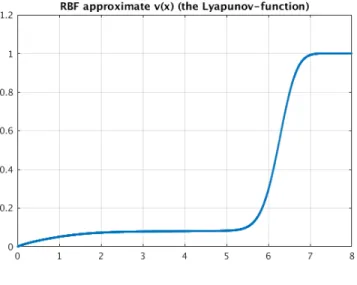
The approximating function v and Lv are displayed in Figure 1. We obtain the values α1 = 653.0140 and α2 = 0.9440. Since in the 1-dimensional case the
boundary values for the approximation are v(ρ1) = 0 and v(ρ2) = 1, we choose a= 1 andb= 0 and henceU = [ρ1, ρ2]. We first use Theorem3.5on any compact
set C with F = F1 = F2 = 1, G = 9/8, G1 = 1.9566, and G2 = 9 to obtain
maxz∈R|(Lv)
00(z)|= 1.6846·1012=:C
U; for the values ψk,l see Table3.
We now use Theorem4.3and chooseh= 2.1307·10−8, which corresponds to 7.5·
108evenly spaced pointsY
U =Ch∩[ρ1−h/2, ρ2+h/2] =h/2Z∩[ρ1−h/2, ρ2+h/2]
on the interval. We obtain a maximum value of maxy∈YULv(y) = −0.281·10
−3 and thus ν= max y∈YU Lv(y) +CU h2 4 =−0.281·10 −3+ 0.19119·10−3<0.
By Theorem4.3,v is a non-local Lyapunov function.
Now we need to determine constants 0< β <1 and 0< λ < α <1, see Theorem
2.5, such that
Figure 1. Above: the computed non-local Lyapunov function v
for system (5.1). Below: the functionLv, approximating−10−3.
Following calculations from [8] we compute a lower estimate [−r1−β, r1−β] for the
(1−β)-BOA of the equilibrium, by solvingU(r1−β) =βUmax. Thusr1−β =β22−1/2.
Theorem2.5requires
which is equivalent to ρ1 = 10−2 < r1−β =β22−1/2, i.e. β >0.1189. We need to
findλsuch that
U−1(Umax)⊂v−1([0, λ])
which is equivalent to V(2−1/2)≤λ. We now fixβ = 0.1247, λ= 0.0421 and we
are free to chooseα > λ.
Corresponding to our choice ofα, we have that the setv−1([0, α])∪ Bis a subset
of theγ-BOA by Theorem2.5(note that b= 0 and a= 1) with
γ=(1−α)(1−β) 1−β(1−λ) .
Forα= 0.044 we haveV−1([0, α])∪ B ≈[−0.803,0.803] andγ≈0.95.
Forα= 0.09 we haveV−1([0, α])∪ B ≈[−5.33,5.33] and γ≈0.90.
Let us compare these results first to the local Lyapunov function: here we obtain [−0.00177,0.00177] and [−0.00707,0.00707] as lower estimates of the 0.95- and 0. 90-BOAs. By comparing those values with the estimates obtained above we see a very substantial increase.
Our results are comparable to the results in [8] in that we obtained similarly sized
γ-BOA, however, our method includes a rigorous verification (numerical proof) that
v is indeed a non-local Lyapunov function. This verification is missing in [8] and one can only hope that the computed non-local function is a Lyapunov function for the system.
Lastly, we set up a simple Monte-Carlo simulation using the First-order stochastic Runge-Kutta method to generate 1000 approximate realizations of sample paths, starting at the pointx= 5.33. We then check when they leave the interval [10−4,8]
and at which end. The result is that 98% of simulations leave through the inner boundary and 2% through the outer, which is close to what we expected since the point 5.33 is inside the 0.9-BOA. Note that this a larger value than predicted by our method. On the one hand, our estimate is indeed just a lower bound and exiting [10−4,8] through the lower boundary is not the same as the sample trajectories
converging to the origin as time tends to infinity. It confirms, however, the validity of our estimate.
5.2. Two-dimensional example. We consider the first example from [3, Section 4], namely
dx = (M +ρ(x)I)xdt+g(x)dW, (5.2) where W is a one-dimensional Wiener-process, I is the 2×2 identity matrix, and with M = 0 1 −1 0 , ρ(x) =kxk −1, andg(x) =θkxk kxk − 1 2 kxk − 3 2 x.
To assert the existence of unique strong solutions we use these formulas forf(x) = (M +ρ(x)I)x and g(x) inside of a ball, centered at the origin and with radius 4 and outside of this ball we extendf andgas Lipschitz functions. For this SDE the generator is L:= 1 2 2 X i,j=1 aij(x) ∂2 ∂xi∂xj + 2 X i=1 fi(x) ∂ ∂xi , where a(x) :=g(x)g(x)>.
(a)The functionvfor system (5.2).
(b)The functionLvfor system (5.2), approximating−10−2.
Figure 2. Non-local Lyapunov function for system (5.2) withθ= 1. The non-local Lyapunov functions looks very similar to the one computed in [3].
By solving the continuous time Lyapunov equationJ>P +P J =−2I for the de-terministic linearised system
x0 =Jx with J = −1 1 −1 −1 =Df(0),
we get the Lyapunov function U(x) = kxk2. For our system this delivers with x= (x, y): U(x) = 1 2θ 2kxk2 kxk −1 2 2 kxk − 3 2 2 x2·2 +xy·0 +yx·0 +y2·2 +[(kxk −1)x+y]·2x+ [−x+ (kxk −1)y]2y = θ2kxk4 kxk −1 2 2 kxk − 3 2 2 + (kxk −1)(2x2+ 2y2) = −kxk2 2−2kxk −θ2kxk2 kxk −1 2 2 kxk − 3 2 2! . Set hθ(r) = 2−2r−θ2r2 r−1 2 2 r−3 2 2 . Then LU(x) = −kxk2h
θ(kxk) and routine calculations show that on the interval
[0,1/2] the function r 7→ r2(r− 1 2)
2(r− 3 2)
2 takes its largest value at r∗ = (4−
√
7)/6 ≈0.22571 and thathθ(r∗)>1.55−6.3·10−3θ2, so for any 0≤θ ≤15.56
the functionU(x) =kxk2 is a Lyapunov function for the system onB
1/2(0). It is
not difficult to verify that if 0 ≤θ ≤1, then U is a (local) Lyapunov function on
B0.9(0).
Now we calculate the constants for K = {x ∈ R2 : R1 ≤ kxk ≤ R2} with R2= 2. We have, see appendix,F =R2
p 1 + (R2−1)2= 2 √ 2,F1= √ 12,F2= 2, G=92θ2,G1= 33θ2, andG2= 197.5θ2.
We used the Wendland function φ8,6 with c = 1, for the system (5.2) with θ = 1. We choose ρ1 = 0.4 and ρ2 = 1.9 and use a 80×80 grid of collocation
points on [−2,2]×[−2,2] to calculate a non-local Lyapunov function, approximating
LV(x) = −10−2, see Figure2. With α
1 = 401.4572 and α2 = 5.8372 we obtain
the valueCU = 4.3220·1012. By evaluatingLV on a relatively coarse 1000×1000
grid of points on [−2,2]×[−2,2], we estimated the maximum value of LV not to exceed−0.005. Hence, we require a checking grid with h= 3.4013·10−8 and thus
we need to evaluateLV at (1.1760·108)2≈1016 points. Our current software and
computer setup is not adequate to complete those calculations in a reasonable time frame, but we note that the verification workload is perfectly parallel which can be used to make the calculations fast. The necessary estimates for these computations are included in the appendix for future reference.
Now similarly to Example 5.1, we have to determine constants 0 < β <1 and 0< λ < α <1 (see Theorem2.5), such that
U−1(Umax)⊂v−1([0, λ]) and ∂B=v−1(0)⊂U−1([0, βUmax]),
whereU(x) =kxk2is the local Lyapunov function onB
1/2(0). We calculate a lower
estimate for the (1−β)-BOA,{x∈R2 : kxk ≤r1−β}, of the equilibrium by choosing B1/2(0) =U−1([0, Umax]), i.e.Umax= 1/4, and solvingBr1−β(0) =U
−1([0, βU max]). Thusr1−β= √ β 2 . Theorem 2.5 requires v−1(0)⊂U−1([0, βUmax])
which is equivalent to 0.4 ≤r1−β = √
β2, i.e. β >0.64. Now we need to findλ
such that
U−1(Umax)⊂v−1([0, λ]).
We now fix β = 0.65, λ= 0.005 and we are free to choose α > λ. Corresponding to our choice of αwe have that the set v−1((0, α)) is a subset of the γ-BOA by
Theorem2.5(withb= 0 anda= 0) with
γ=(1−α)(1−β) 1−β(1−λ) .
Forα= 0.01 we havev−1([0, α])∪ B ≈B
0.6454(0) andγ≈0.9809
Forα= 0.09 we havev−1([0, α])∪ B ≈B0.839(0) andγ≈0.90.
Let us compare these results to the local Lyapunov function: Here we obtain
B0.0707(0) and B0.1581(0) as lower estimates of the 0.98 and 0.90-BOAs. By
com-paring the estimates above we see a substantial increase.
Our results are comparable to the results in [3] in that we obtained similarly sizedγ-BOA. However, our method includes a framework for rigorous verification (numerical proof) that v is indeed a non-local Lyapunov function, although this verification could not be performed at this point due to its huge computational demand.
Acknowledgement
This research and, in particular, Bj¨ornsson and Gudmundsson were supported by The Icelandic Research Fund with the project Lyapunov Methods and Stochastic Stability (grant nr. 152429-051).
AppendixA. Explicit formulas for meshless collocation. We calculatev(x),
Lv(x), and the collocation matrixA for the specific operatorLgiven in (3.3). We denote recursivelyψi+1(r) = 1r∂r∂ ψi(r) fori= 0,1, . . . ,5 andψ0=ψ, whereψis a
certain Wendland functions that can be found below in Tables1and2. Recall that
k · k=k · k2.
We have, see (3.5), that
v(x) = N X k=1 αk −ψ1(kx−xkk)hx−xk, f(xk)i +1 2 d X i,j=1 mij(xk)[ψ2(kx−xkk)(x−xk)i(x−xk)j +δijψ1(kx−xkk)] + M X k=1 αN+kψ0(kx−ξkk). (A.1)
The formula forLv(x) is, abbreviatingβ=x−xk, Lv(x) = N X k=1 αk −ψ2(kβk)hβ, f(x)ihβ, f(xk)i −ψ1(kβk)hf(x), f(xk)i +1 2 d X i,j=1 mij(xk) ψ3(kβk)hβ, f(x)iβiβj+ψ2(kβk)fj(x)βi +ψ2(kβk)fi(x)βj+δijψ2(kβk)hβ, f(x)i +1 2 d X i,j=1 mij(x) −ψ3(kβk)hβ, f(xk)iβiβj−ψ2(kβk)fj(xk)βi −ψ2(kβk)fi(xk)βj−δijψ2(kβk)hβ, f(xk)i +1 4 d X r,s=1 d X i,j=1 mrs(x)mij(xk) ψ4(kβk)βiβjβrβs +ψ3(kβk)[δijβrβs+δirβjβs +δisβjβr+δjrβiβs+δjsβiβr+δrsβiβj] +ψ2(kβk)[δijδrs+δirδjs+δisδjr] + M X k=1 αN+k −ψ1(kξk−xk)hξk−x, f(x)i +1 2 d X i,j=1 mij(x)[ψ2(kξk−xk)(ξk−x)i(ξk−x)j +δijψ1(kξk−xk)].
The formulas for the matrix elements are
dkl = ψ0(kξk−ξlk), ckl = −ψ1(kξl−xkk)hξl−xk, f(xk)i +1 2 d X i,j=1 mij(xk)[ψ2(kξl−xkk)(ξl−xk)i(ξl−xk)j +δijψ1(kξl−xkk)],
and, abbreviatingβ=xk−xl, bkl = −ψ2(kβk)hβ, f(xk)ihβ, f(xl)i −ψ1(kβk)hf(xk), f(xl)i +1 2 d X i,j=1 mij(xl) ψ3(kβk)hβ, f(xk)iβiβj+ψ2(kβk)fj(xk)βi +ψ2(kβk)fi(xk)βj+δijψ2(kβk)hβ, f(xk)i +1 2 d X i,j=1 mij(xk) −ψ3(kβk)hβ, f(xl)iβiβj−ψ2(kβk)fj(xl)βi −ψ2(kβk)fi(xl)βj−δijψ2(kβk)hβ, f(xl)i +1 4 d X r,s=1 d X i,j=1 mrs(xk)mij(xl) ψ4(kβk)βiβjβrβs +ψ3(kβk)[δijβrβs+δirβjβs+δisβjβr +δjrβiβs+δjsβiβr+δrsβiβj] +ψ2(kβk)[δijδrs+δirδjs+δisδjr] .
Appendix B. Two-dimensional example. In this section we give the details of the estimates forFi andGi of the 2-dimensional example from Section5.2.
Withf(x1, x2) = (kxk −1)x1+x2 −x1+ (kxk −1)x2 we obtain F = (kxk −1)2x21+x22+ 2x1x2(kxk −1) +x21−2x1x2(kxk −1) +x22(kxk −1)2 1/2 = kxkp(kxk −1)2+ 1,
∂f ∂x1 = x2 1 kxk+kxk −1 −1 +x1x2 kxk ! = 2x2 1+x22 kxk −1 −1 +x1x2 kxk ! , ∂f ∂x2 = x1x2 kxk + 1 x22 kxk+kxk −1 ! = x1x2 kxk + 1 x21+2x22 kxk −1 ! , ∂f ∂x2 2 = x 2 1x22+x41+ 4x21x22+ 4x42 kxk2 + 2x1x2−2x21−4x22 kxk + 2 ≤ x21+ 4x22−x 2 1+ 3x22 kxk + 2 = x21 1− 1 kxk +x22 4− 3 kxk + 2 ≤ x21 1− 1 R2 +x22 4− 3 R2 + 2 ≤ R22max 0, 1− 1 R2 , 4− 3 R2 + 2, ∂2f ∂x2 1 = x1(2x21+3x 2 2) kxk3 x32 kxk3 , ∂2f ∂x1∂x2 = x3 2 kxk3 x3 1 kxk3 , ∂2f ∂x2 2 = x3 1 kxk3 x2(3x21+2x22) kxk3 , and ∂2f ∂x2 2 = p x6 1+ 9x41x22+ 12x21x42+ 4x62 kxk3 ≤ p 4x61+ 12x41x22+ 12x21x42+ 4x62 kxk3 = p 4(x2 1+x22)3 kxk3 = 2.
We now calculate the estimates forg(x) =θr(r−0.5)(r−1.5)x, denotingkxk=r. Forr∈[0,2] we have kg(x)k ≤ θ4· 3 2· 1 2 = 3θ. Furthermore, ∂g ∂xi = θ x i kxk 3r2−4r+3 4 x+r(r−0.5)(r−1.5)ei Hence, ∂g ∂xi ≤ θ 3r2−4r+3 4 r+|r(r−0.5)(r−1.5)| ≤ 11θ
forr∈[0,2]. Finally, ∂2g ∂x2 1 = θ 3r2−4r+3 4 x22 kxk3x+ 2 x1 kxke1 +θ x 2 1 kxk2(6r−4)x = θ r3 3r2−4r+3 4 x22+ (6r2−4r)x21 x +2θ 3r2−4r+3 4 x 1 kxke1, ∂2g ∂x2 1 ≤ θmax 3r2−4r+3 4 ,6r2−4r +2θ 3r2−4r+3 4 ≤ 25.5θ forr∈[0,2], ∂2g ∂x1∂x2 = θ 3r2−4r+3 4 −x1x2 kxk3 x+ x2 kxke1+ x1 kxke2 +θx1x2 kxk2(6r−4)x = θ r3 −3r2+ 4r−3 4+ 6r 2 −4r x1x2x +θ r 3r2−4r+3 4 (x2e1+x1e2), and ∂2g ∂x1∂x2 ≤ θ 3r2−3 4 +θ 3r2−4r+3 4 ≤ 16θ.
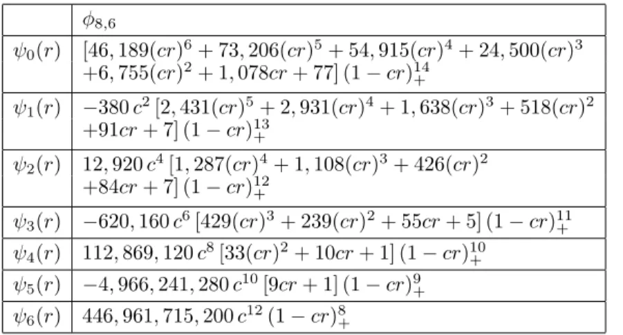
Appendix C. Wendland functions. In this appendix we give the explicit for-mulas of the Wendland functionsφ8,6 and φ7,6 as well as the corresponding
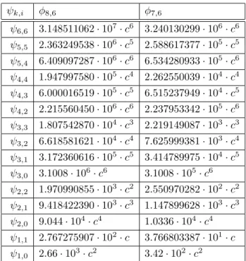
aux-iliary functions ψi, i = 1, . . . ,6. Furthermore, we give the relevant estimates for ψk,i= supr∈[0,∞)|ψk(r)|ri.
In particular, in Table1and Table2, we give the formulas for the Wendland func-tionψ0(r) =φ8,6(cr) andψ0(r) =φ7,6(cr), respectively, as well asψi,i= 1, . . . ,6.
In Table 3 we give the formulas for the expressions ψk,i = supr∈[0,∞)ψk(r)ri,
re-quired for the estimates for the same Wendland functionsφ8,6 andφ7,6. Note that x+:= max{x,0}.
REFERENCES
[1] H. Bj¨ornsson, P. Giesl, S. Gudmundsson, and S. Hafstein. Local Lyapunov functions for nonlinear stochastic differential equations by linearization. InProceedings of the 15th International Conference on Informatics in Control, Automation and Robotics (ICINCO 2018) -Volume 1, pages 579–586, 2018.
[2] M. Buhmann.Radial basis functions: theory and implementations, volume 12 ofCambridge Monographs on Applied and Computational Mathematics. Cambridge University Press, Cam-bridge, 2003.
[3] F. Camilli and L. Gr¨une. Characterizing attraction probabilities via the stochastic Zubov equation.Discrete Contin. Dyn. Syst. Ser. B, 3(3):457–468, 2003.
[4] P. Giesl. Construction of global Lyapunov functions using Radial Basis Functions, volume 1904 ofLecture Notes in Mathematics. Springer, Berlin, 2007.
φ8,6 ψ0(r) [46,189(cr)6+ 73,206(cr)5+ 54,915(cr)4+ 24,500(cr)3 +6,755(cr)2+ 1,078cr+ 77] (1−cr)14 + ψ1(r) −380c2[2,431(cr)5+ 2,931(cr)4+ 1,638(cr)3+ 518(cr)2 +91cr+ 7] (1−cr)13+ ψ2(r) 12,920c4[1,287(cr)4+ 1,108(cr)3+ 426(cr)2 +84cr+ 7] (1−cr)12+ ψ3(r) −620,160c6[429(cr)3+ 239(cr)2+ 55cr+ 5] (1−cr)11+ ψ4(r) 112,869,120c8[33(cr)2+ 10cr+ 1] (1−cr)10+ ψ5(r) −4,966,241,280c10[9cr+ 1] (1−cr)9+ ψ6(r) 446,961,715,200c12(1−cr)8+
Table 1. The table shows the Wendland function ψ0(r) := φ8,6(cr) as well as the related functions ψ1 to ψ6, defined
recur-sively byψk+1(r) := ∂rψrk(r) fork= 0,1, . . . ,5. φ7,6 ψ0(r) [4,096(cr)6+ 7,059(cr)5+ 5,751(cr)4+ 2,782(cr)3+ 830(cr)2 +143cr+ 11] (1−cr)13 + ψ1(r) −38c2[2,048(cr)5+ 2,697(cr)4+ 1,644(cr)3+ 566(cr)2 +108cr+ 9] (1−cr)12 + ψ2(r) 10,336c4[128(cr)4+ 121(cr)3+ 51(cr)2+ 11cr+ 1] (1−cr)11+ ψ3(r) −62,016c6[320(cr)3+ 197(cr)2+ 50cr+ 5] (1−cr)10+ ψ4(r) 3,224,832c8[80(cr)2+ 27cr+ 3] (1−cr)9+ ψ5(r) −354,731,520c10[8cr+ 1] (1−cr)8+ ψ6(r) 25,540,669,440c12(1−cr)7+
Table 2. The table shows the Wendland function ψ0(r) := φ7,6(cr) as well as the related functions ψ1 to ψ6, defined
recur-sively byψk+1(r) :=
∂rψk(r)
r fork= 0,1, . . . ,5.
[5] P. Giesl and S. Hafstein. Review of computational methods for Lyapunov functions.Discrete Contin. Dyn. Syst. Ser. B, 20(8):2291–2331, 2015.
[6] P. Giesl and N. Mohammed. Verification estimates for the construction of Lyapunov functions using meshfree collocation. Discrete Contin. Dyn. Syst. Ser. B, in press.
[7] P. Giesl and H. Wendland. Meshless collocation: Error estimates with application to dynam-ical systems.SIAM J. Numer. Anal., 45(4):1723–1741, 2007.
[8] S. Gudmundsson and S. Hafstein. Probabilistic basin of attraction and its estimation using two Lyapunov functions.Complexity, Article ID:2895658, 2018.
[9] S. Hafstein, S. Gudmundsson, P. Giesl, and E. Scalas. Lyapunov function computation for au-tonomous linear stochastic differential equations using sum-of-squares programming.Discrete Contin. Dyn. Syst. Ser. B, 2(23):939–956, 2018.
[10] N. Mohammed.Grid refinement and verification estimates for the RBF construction method of Lyapunov functions. PhD thesis, University of Sussex, 2016.
ψk,i φ8,6 φ7,6 ψ6,6 3.148511062·107·c6 3.240130299·106·c6 ψ5,5 2.363249538·106·c5 2.588617377·105·c5 ψ5,4 6.409097287·106·c6 6.534280933·105·c6 ψ4,4 1.947997580·105·c4 2.262550039·104·c4 ψ4,3 6.000016519·105·c5 6.515237949·104·c5 ψ4,2 2.215560450·106·c6 2.237953342·105·c6 ψ3,3 1.807542870·104·c3 2.219149087·103·c3 ψ3,2 6.618581621·104·c4 7.625999381·103·c4 ψ3,1 3.172360616·105·c5 3.414789975·104·c5 ψ3,0 3.1008·106·c6 3.1008·105·c6 ψ2,2 1.970990855·103·c2 2.550970282·102·c2 ψ2,1 9.418422390·103·c3 1.147899628·103·c3 ψ2,0 9.044·104·c4 1.0336·104·c4 ψ1,1 2.767275907·102·c 3.766803387·101·c ψ1,0 2.66·103·c2 3.42·102·c2
Table 3. The table shows values for ψk,i := supr∈[0,∞)|ψi(r)|rk
for the Wendland functionsψ0(r) :=φ8,6(cr) andψ0(r) :=φ7,6(cr).
[11] M. J. D. Powell. The theory of radial basis function approximation in 1990. In Advances in numerical analysis, Vol. II (Lancaster, 1990), Oxford Sci. Publ., pages 105–210. Oxford Univ. Press, New York, 1992.
[12] R. Schaback and H. Wendland. Kernel techniques: from machine learning to meshless meth-ods.Acta Numer., 15:543–639, 2006.
[13] H. Wendland. Error estimates for interpolation by compactly supported radial basis functions of minimal degree.J. Approx. Theory, 93(2):258–272, 1998.
[14] H. Wendland.Scattered Data Approximation, volume 17 ofCambridge Monographs on Applied and Computational Mathematics. Cambridge University Press, Cambridge, 2005.
E-mail address:[email protected]
E-mail address:[email protected]
E-mail address:[email protected]
E-mail address:[email protected]