†Computer Sciences Dept. University of Wisconsin-Madison
Madison, WI 53706, USA {goldberg,jerryzhu,zhiting}
@cs.wisc.edu
Andrew B. Goldberg† Xiaojin Zhu† Aarti Singh‡ Zhiting Xu† Robert Nowak∗ ‡Applied and Computational Math
Princeton University Princeton, NJ 08544, USA
∗Elec. and Computer Engineering University of Wisconsin-Madison
Madison, WI 53706, USA [email protected]
Abstract
We study semi-supervised learning when the data consists of multiple intersecting mani-folds. We give a finite sample analysis to quantify the potential gain of using unlabeled data in this multi-manifold setting. We then propose a semi-supervised learning algorithm that separates different manifolds into deci-sion sets, and performs supervised learning within each set. Our algorithm involves a novel application of Hellinger distance and size-constrained spectral clustering. Exper-iments demonstrate the benefit of our multi-manifold semi-supervised learning approach.
1
INTRODUCTION
The promising empirical success of semi-supervised learning algorithms in favorable situations has trig-gered several recent attempts (Balcan & Blum 2005, Ben-David, Lu & Pal 2008, Kaariainen 2005, Laf-ferty & Wasserman 2007, Niyogi 2008, Rigollet 2007) at developing a theoretical understanding of semi-supervised learning. In a recent paper (Singh, Nowak & Zhu 2008), it was established using a finite sam-ple analysis that if the comsam-plexity of the distribu-tions under consideration is too high to be learnt us-ing n labeled data points, but is small enough to be learnt using m n unlabeled data points, then semi-supervised learning (SSL) can improve the per-formance of a supervised learning (SL) task. There have also been many successful practical SSL algo-rithms as summarized in (Chapelle, Zien & Sch¨olkopf 2006, Zhu 2005). These theoretical analyses and prac-Appearing in Proceedings of the 12th International Confe-rence on Artificial Intelligence and Statistics (AISTATS) 2009, Clearwater Beach, Florida, USA. Volume 5 of JMLR: W&CP 5. Copyright 2009 by the authors.
tical algorithms often assume that the data forms clus-ters or resides on a single manifold.
However, both a theory and an algorithm are lacking when the data is supported on a mixture of manifolds. Such data occurs naturally in practice. For instance, in handwritten digit recognition each digit forms its own manifold in the feature space; in computer vision motion segmentation, moving objects trace different trajectories which are low dimensional manifolds (Tron & Vidal 2007). These manifolds may intersect or par-tially overlap, while having different dimensionality, orientation, and density. Existing SSL approaches can-not be directly applied to multi-manifold data. For instance, traditional graph-based SSL algorithms may create a graph that connects points on different mani-folds near a manifold intersection, thus diffusing infor-mation across the wrong manifolds.
In this paper, we generalize the theoretical analysis of (Singh et al. 2008) to the case where the data is sup-ported on a mixture of manifolds. Guided by the the-ory, we propose an SSL algorithm that handles multi-ple manifolds as well as clusters. The algorithm builds upon novel Hellinger-distance-based graphs and size-constrained manifold clustering. Experiments show that our algorithm can perform SSL on multiple in-tersecting, overlapping, and noisy manifolds.
2
THEORETIC PERSPECTIVES
In this section, we first review the conclusions of (Singh et al. 2008), which are based on the cluster assump-tion, and then give conjectured bounds in the single manifold and multi-manifold case.
The cluster assumption, as formulated in (Singh et al. 2008), states that the target regression function or class label is locally smooth over certain subsets of theD-dimensional feature space that are delineated by changes in the marginal density—throughout this pa-per, we assume the marginal density is bounded above
and below (away from zero). We refer to these delin-eated subsets as decision sets; i.e., all non-empty sets formed by intersections between the cluster support sets and their complements. If these decision sets, de-noted by C, can be learnt using unlabeled data, the learning task on each decision set is simplified. The results of (Singh et al. 2008) suggest that if the de-cision sets can be resolved using unlabeled data, but not using labeled data, then semi-supervised learning can help. However, this simple argument, and hence the distinctions between SSL and SL, are not always captured by standard asymptotic arguments based on rates of convergence. (Singh et al. 2008) used finite sample bounds to characterize both the SSL gains and the relative value of unlabeled data.
To derive the finite sample bounds, the first step is to understand when the decision sets are resolvable using data. This depends on the interplay between the complexity of the class of distributions under con-sideration and the number of unlabeled pointsmand labeled points n. For the cluster case, the complex-ity of the distributions is determined by the margin
γ, defined as the minimum separation between clus-ters or the minimum width of a decision set (Singh et al. 2008). If the margin γ is larger than the typi-cal distance between the data points (m−1/D if using unlabeled data, or n−1/D if using only labeled data), then with high probability the decision sets can be learnt up to a high accuracy (which depends on mor
n, respectively) (Singh et al. 2008). This implies that
if γ > m−1/D (margin exists with respect to density
ofunlabeled data), then the finite sample performance (the expected excess error Err) of a semi-supervised learnerfbm,n relative to the performance of a clairvoy-ant supervised learner fbC,n, which has perfect knowl-edge of the decision sets C, can be characterized as follows: sup PXY(γ) Err(fbm,n) ≤ sup PXY(γ) Err(fbC,n) +δ(m, n). (1) HerePXY(γ) denotes the cluster-based class of distri-butions with complexityγ, andδ(m, n) is the error in-curred due to inaccuracies in learning the decision sets using unlabeled data. Comparing this upper bound on the semi-supervised learning performance to a fi-nite sample minimax lower bound on the performance of any supervised learner provides a sense of the rel-ative performance of SL vs. SSL. Thus, SSL helps if complexity of the class of distributions γ > m−1/D and both of the following conditions hold: (i) knowl-edge of decision sets simplifies the supervised learn-ing task, that is, the error of the clairvoyant learner supPXY(γ)Err(fbC,n) < inffnsupPXY(γ)Err(fn), the
smallest error that can be achieved by any supervised learner based onnlabeled data. The difference
quan-Table 1: Conjectured finite sample performance of SSL and SL for regression of a H¨older-α, α > 1, smooth function (with respect to geodesic distance in the man-ifold cases). These bounds hold for D ≥ 2, d < D,
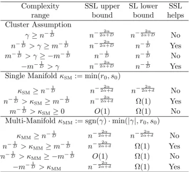
mn, and suppress constants and log factors. Complexity SSL upper SL lower SSL
range bound bound helps
Cluster Assumption γ≥n−D1 n− 2α 2α+D n−2α2+αD No n−D1 > γ≥m− 1 D n− 2α 2α+D n−D1 Yes m−D1 > γ≥ −m− 1 D n− 1 D n− 1 D No −m−D1 > γ n− 2α 2α+D n−D1 Yes
Single ManifoldκSM:= min(r0, s0)
κSM≥n− 1 D n− 2α 2α+d n− 2α 2α+d No n−D1 > κSM≥m− 1 D n− 2α 2α+d Ω(1) Yes m−D1 > κSM≥0 O(1) Ω(1) No Multi-Manifold κMM:= sgn(γ)·min(|γ|, r0, s0) κMM≥n− 1 D n− 2α 2α+d n− 2α 2α+d No n−D1 > κMM≥m− 1 D n− 2α 2α+d Ω(1) Yes m−D1 > κMM≥ −m−D1 O(1) Ω(1) No −m−1 D > κMM n− 2α 2α+d Ω(1) Yes
tifies the SSL performance gain. (ii)mis large enough so that the error incurred due to using a finite amount of unlabeled data to learn the decision sets is negligi-ble: δ(m, n) = OsupPXY(γ)Err(fbC,n)
. This quan-tifies the relative value of labeled and unlabeled data. The finite sample performance bounds on SSL and SL performance as derived in (Singh et al. 2008) for the cluster assumption are summarized in Table 1 for the regression setting, where the target function is a H¨older-α smooth function on each decision set and
α > 1. We can see that SSL provides improved
per-formance, by capitalizing on the local smoothness of the function on each decision set, when the separation between the clusters is large compared to the typical distance between unlabeled datam−1/D but less than the typical distance between labeled datan−1/D. Neg-ative γ refers to the case where the clusters are not separated, but can overlap and give rise to decision sets that are adjacent (see (Singh et al. 2008)). In this case, SSL always outperforms SL provided the width of the resulting decision sets is detectable using unla-beled data. Thus, the interplay between the margin and the number of labeled and unlabeled data charac-terizes the relative performance of SL vs. SSL under the cluster assumption. Similar results can be derived in the classification setting where an exponential im-provement (from n−1/D to e−n) is possible provided the number of unlabeled data mgrows exponentially
withn(Singh et al. 2008).
2.1 SINGLE MANIFOLD CASE
In the single manifold case, the assumption is that the target function lies on a lowerd-dimensional man-ifold, where d < D, and is H¨older-αsmooth (α >1) with respect to the geodesic distance on the manifold. Hence knowledge of the manifold, or equivalently the geodesic distances between all pairs of data points, can be gleaned using unlabeled data and reduces the di-mensionality of the learning task.
In the case of distributions supported on a single man-ifold, the ability to learn the geodesic distances well, and hence the complexityκSMof the distributions, de-pends on two geometric properties of the manifold— its minimum radius of curvature r0 and proximity to
self-intersection s0 (also known as branch separation)
(Bernstein, de Silva, Langford & Tenenbaum 2000). If κSM := min(r0, s0) is larger than the typical
dis-tance between the data points (m−1/Dwith unlabeled data, orn−1/Dwith only labeled data), then with high probability the manifold structure is resolvable and geodesic distances can be learnt up to a high accuracy (which depends onmor n, respectively). This can be achieved by using shortest distance paths on an - or
k-nearest neighbor graph to approximate the geodesic distances (Bernstein et al. 2000). The use of approx-imate geodesic distances to learn the target function gives rise to an error-in-variable problem. Though the overall learning problem is now reduced to a lower-dimensional problem, we are now faced with two types of errors—the label noise and the error in the esti-mated distances. However, the error incurred in the final estimation due to errors in geodesic distances de-pends onmwhich is assumed to be much greater than
n. Thus, the effect of the geodesic distance errors is negligible, compared to the error due to label noise, for m sufficiently large. This suggests that for the manifold case, if κSM > m−1/D, then finite sample performance of semi-supervised learning can again be related to the performance of a clairvoyant supervised learnerfbC,nas in (1) above, sinceδ(m, n) is negligible
formsufficiently large.
Comparing this SSL performance bound to a finite sample minimax lower bound on the performance of any supervised learner indicates SSL’s gain in the sin-gle manifold case and is summarized in Table 1. These are conjectured bounds based on the arguments above and similar arguments in (Niyogi 2008). The SSL up-per bound can be achieved using a learning procedure adaptive to bothαandd, such as the method proposed in (Bickel & Li 2007)1. The SL lower bounds follow
1
Note, however, that the analysis in (Bickel & Li 2007)
from the results in (Tsybakov 2004) and (Niyogi 2008). SSL provides improved performance by capitalizing on the lower-dimensional structure of the manifold when the minimum radius of curvature and branch separa-tion are large compared to the typical distance be-tween unlabeled data m−1/D, but small compared to
the typical distance between labeled datan−1/D. 2.2 MULTI-MANIFOLD CASE
The multi-manifold case addresses the generic setting where the clusters are low-dimensional manifolds that possibly intersect or overlap. In this case, the target function is supported on multiple manifolds and can be piecewise smooth on each manifold. Thus, it is of in-terest to resolve the manifolds, as well as the subsets of each manifold where the decision label varies smoothly (that are characterized by changes in the marginal den-sity). The analysis for this case is a combination of the cluster and single manifold case. The complexity of the multi-manifold class of distributions, denoted κMM, is governed by the minimum of the manifold curvatures, branch separations, and the separations and overlaps between distinct manifolds. For the regression setting, the conjectured finite sample minimax analysis is pre-sented in Table 1.
These results indicate that when there is enough unla-beled data, but not enough launla-beled data, to handle the complexity of the class, then semi-supervised learning can help by adapting to both the intrinsic dimensional-ity and smoothness of the target function. Extensions of these results to the classification setting are straight-forward, as discussed under the cluster assumption.
3
AN ALGORITHM
Guided by the theoretical analysis in the previous sec-tion, we propose a “cluster-then-label” type of SSL al-gorithm, see Figure 1. It consists of three main steps: (1) It uses the unlabeled data to form a small num-ber of decision sets, on which the target function is assumed to be smooth. The decision sets are defined in the ambient space, not just on the labeled and unla-beled points. (2) The target function within a partic-ular decision set is estimated using only labeled data that fall in that decision set, and using a supervised learner specified by the user. (3) a new test point is predicted by the target function in the decision set it falls into.
There have been several cluster-then-label approaches in the SSL literature. For example, the early work of Demiriz et al. modifies the objective of standard
considers the asymptotic performance of SL, whereas here we are studying the finite-sample performance of SSL.
k-means clustering algorithms to include a class impu-rity term (Demiriz, Bennett & Embrechts 1999). El-Yaniv and Gerzon enumerate all spectral clusterings of the unlabeled data with varying number of clusters, which together with labeled data induce a hypothesis space. They then select the best hypothesis based on an Occam’s razor-type transductive bound (El-Yaniv & Gerzon 2005). Some work in “constrained cluster-ing” is also closely related to cluster-then-label from an SSL perspective (Basu, Davidson & Wagstaff 2008). Compared to these approaches, our algorithm has two advantages: i) it is supported by our SSL minimax theory; ii) it handles both overlapping clusters and in-tersecting manifolds by detecting changes in support, density, dimensionality or orientation.
Our algorithm is also different from the family of graph-regularized SSL approaches, such as manifold regularization (Belkin, Sindhwani & Niyogi 2006) and earlier variants (Joachims 2003, Zhou, Bousquet, Lal, Weston & Sch¨olkopf 2004, Zhu, Ghahramani & Lafferty 2003). Those approaches essentially add a graph-regularization term in the objective. They also depend on the “manifold assumption” that the target function indeed varies smoothly on the manifold. In contrast, i) our algorithm is awrapper method, which uses any user-specified supervised learnerSLas a sub-routine. This allows us to directly take advantage of advances in supervised learning without the need to derive new algorithms. ii) Our theory ensures that, even when the manifold assumption is wrong, our SSL performance bound is the same as that of the super-vised learner (up to a log factor).
Finally, step 1 of our algorithm is an instance of man-ifold clustering. Recent advances on this topic include Generalized Principal Component Analysis (Vidal, Ma & Sastry 2008) and lossy coding (Ma, Derksen, Hong & Wright 2007) for mixtures of linear subspaces, mul-tiscale manifold identification with algebraic multi-grid (Kushnir, Galun & Brandt 2006), tensor vot-ing (Mordohai & Medioni 2005), spectral curvature clustering (Chen & Lerman 2008), and translated Pois-son mixture model (Haro, Randall & Sapiro 2008) for mixtures of nonlinear manifolds. Our algorithm is unique in two ways: i) its use of Hellinger distance offers a new approach to detecting overlapping clus-ters and inclus-tersecting manifolds; ii) our decision sets have minimum size constraints, which we enforce by constrained k-means.
3.1 HELLINGER DISTANCE GRAPH
Let the labeled data be {(xi, yi)}n
i=1, and the
unla-beled data be {xj}M
j=1, where M n. The
build-ing block of our algorithm is a local sample covari-ance matrix. For a point x, define N(x) to be
a small neighborhood around x in Euclidean space. Let Σx be the local sample covariance matrix at x:
Σx=Px0∈N(x)(x0−µx)(x0−µx)>/(|N(x)| −1), where µx = Px0∈N(x)x0/|N(x)| is the neighborhood mean. In our experiments, we let|N(x)| ∼O(log(M)) so that the neighborhood size grows with unlabeled data size
M. The covariance Σx captures the local geometry
aroundx.
Our intuition is that points xi, xj on different man-ifolds or in regions with different density should be considered dissimilar. This intuition is captured by the Hellinger distance between their local sample co-variance matrices Σi,Σj. The squared Hellinger
dis-tance is defined between two pdf’s p, q: H2(p, q) = 1 2 R p p(x)−p q(x) 2 dx. By setting p(x) =
N(x; 0,Σi), i.e., a Gaussian with zero mean and
co-variance Σi, and similarly q(x) =N(x; 0,Σj), we
ex-tend the definition of Hellinger distance to covariance matrices: H(Σi,Σj) ≡ H(N(x; 0,Σi),N(x; 0,Σi)) = p
1−2D/2|Σi|1/4|Σ
j|1/4/|Σi+ Σj|1/2, whereD is the
dimensionality of the ambient feature space. We will also callH(Σi,Σj) the Hellinger distance between the
two pointsxi, xj. When Σi+ Σj is rank deficient,His
computed in the subspace occupied by Σi+ Σj. The
Hellinger distance H is symmetric and in [0,1]. H
is small when the local geometry is similar, and large when there is significant difference in density, manifold dimensionality or orientation. Example 3D covariance matrices and theirH values are shown in Figure 2.
Cov. matrices Comment H(Σ1,Σ2)
similar 0.02 density 0.28 dimension 1 orientation 1 Figure 2: Hellinger distance
It would seem natural to compute all pairwise Hellinger distances between our dataset of n +M
points to form a graph, and apply a graph-cut algo-rithm to separate multiple manifolds or clusters. How-ever, ifxi andxjare very close to each other, their lo-cal neighborhoods N(xi), N(xj) will strongly overlap. Then, even if the two points are on different manifolds the Hellinger distance will be small, because their co-variance matrices Σi,Σjwill be similar. Therefore, we
select a subset ofm∼O(M/log(M)) unlabeled points so that they are farther apart while still covering the whole dataset. This is done using a greedy procedure,
Givennlabeled examples andM unlabeled examples, and a supervised learnerSL, 1. Use the unlabeled data to inferk∼O(log(n)) decision setscCi:
(a) Select a subset ofm < M unlabeled points
(b) Form a graph on then+m labeled and unlabeled points, where the edge weights are computed from the Hellinger distance between local sample covariance matrices
(c) Perform size-constrained spectral clustering to cut the graph into k parts, while keeping enough labeled and unlabeled points in each part
2. Use the labeled data incCiand the supervised learningSLto trainfib
3. For test pointx∗∈cCi, predictfi(xb
∗ ).
Figure 1: The Multi-Manifold Semi-Supervised Learning Algorithm
where we first select an arbitrary unlabeled pointx(0).
We then remove its unlabeled neighbors N(x(0)),
in-cluding itself. We select x(1) to be the next nearest neighbor, and repeat. This procedure thus approxi-mately selects a cover of the dataset. We focus on the subset ofmunlabeled andnlabeled points. Each of thesen+mpoints has its local covariance Σ com-puted from the original full dataset. We then discard theM −m unselected unlabeled points. Notice, how-ever, that the number m of effective unlabeled data points is polynomially of the same order as the total number M of available unlabeled data points.
(a) (b)
Figure 3: The graph on the dollar sign dataset. We can now define a sparse graph on then+mpoints. Each point xis connected by a weighted, undirected edge toO(log(n+m)) of its nearest Mahalanobis neigh-bors chosen from the the set ofn+mpoints too. The choice of O(log(n+m)) allows neighborhood size to grow with dataset size. Since we know the local geom-etry around x(captured by Σx), we “follow the
man-ifold” by using the Mahalanobis distance as the local distance metric atx: d2
M(x, x0) = (x−x0)>Σ−x1(x−x0).
For example, a somewhat flat Σx will preferentially
connect to neighbors in or near the same flat sub-space. The graph edges are weighted using the stan-dard RBF scheme, but with Hellinger distance: wij = exp −H2(Σi,Σ
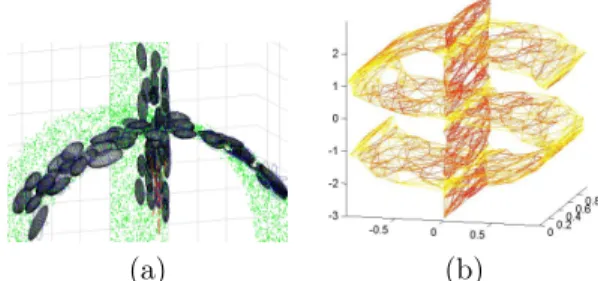
j)/(2σ2). Figure 3(a) shows a small
part of a synthetic “dollar sign” dataset, consisting of two intersecting manifolds: “S” and “|”. The green dots are the original unlabeled points, and the ellip-soids are the contours of covariance matrices around
the subset of selected unlabeled points within a small region. Figure 3(b) shows the graph on the complete dollar sign dataset, where red edges have large weights and yellow edges have small weights. Thus the graph combines locality and geometry: an edge has large weight when the two nodes are close in Mahalanobis distance, and have similar covariance structure.
3.2 SIZE-CONSTRAINED SPECTRAL CLUSTERING
We perform spectral clustering on this graph ofn+m
nodes. We hope each resulting cluster represents a separate manifold, from which we will define a deci-sion set. Of the many spectral clustering algorithms, we chose ratio cut for its simplicity, though others can be similarly adapted for use here. The standard ra-tio cut algorithm for k clusters has four steps (von Luxburg 2007): 1. Compute the unnormalized graph LaplacianL=Deg−W, whereW = [wij] is the weight matrix, andDegii=P
jwij form the diagonal degree
matrix. 2. Compute the k eigenvectorsv1. . . vk ofL
with the smallest eigenvalues. 3. Form matrix V with
v1. . . vk as columns. Use the ith row ofV as the new representation of xi. 4. Cluster all x under the new representation intok clusters using k-means.
Our ultimate goal of semi-supervised learning poses new challenges; we want our SSL algorithm to de-grade gracefully, even when the manifold assumption does not hold. The SSL algorithm should not break the problem into too many subproblems and increase the complexity of the supervised learning task. This is achieved by requiring that the algorithm does not generate too many clusters and that each cluster con-tains “enough” labeled points. Because we will simply do supervised learning within each decision set, as long as the number of sets does not grow polynomially with
n, the performance of our algorithm is guaranteed to be polynomially no worse than the performance of the supervised learner when the manifold assumption fails. Thus, we automatically revert to the supervised
learn-ing performance. One way to achieve this is to have three requirements: i) the number of clusters grows as k ∼O(log(n)); ii) each cluster must have at least
a ∼ O(n/log2(n)) labeled points; iii) each spectral cluster must have at least b ∼ O(m/log2(n)) unla-beled points. The first sets the number of clusters k, allowing more clusters and thus handling more com-plex problems as labeled data size grows, while suffer-ing only a logarithmic performance loss compared to a supervised learner if the manifold assumption fails. The second requirement ensures that each decision set has O(n) labeled points up to log factor2. The third is similar, and makes spectral clustering more robust. Spectral clustering with minimum size constraintsa, b
on each cluster is an open problem. Directly en-forcing these constraints in graph partitioning leads to difficult integer programs. Instead, we enforce the constraints in k-means (step 4) of spectral clus-tering. Our approach is a straightforward extension to the constrained k-means algorithm of Bradley et al. (Bradley, Bennett & Demiriz 2000). For point xi,
let Ti1. . . Tik ∈ R be its cluster indicators: ideally,
Tih = 1 if xi is in cluster h, and 0 otherwise. Let
c1. . . ck ∈Rd denote the cluster centers. Constrained k-means is the iterative minimization overT and cof the following problem:
min T ,c Pn+m i=1 Pk h=1Tihkxi−chk2 s.t. Pk h=1Tih= 1, T ≥0 Pn i=1Tih≥a, Pn+m i=n+1Tih≥b, h= 1. . . k,(2) where we assume the points are ordered so that the first n points are labeled. Fixing T, optimizing over
c is trivial, and amounts to moving the centers to the cluster means.
Bradley et al. showed that fixing c and optimizing T
can be converted into a Minimum Cost Flow problem, which can be exactly solved. In a Minimum Cost Flow problem, there is a directed graph where each node is either a “supply node” with a number r > 0, or a “demand node” with r <0. The arcs from i →j is associated with cost sij, and flow tij. The goal is to
find the flow t such that supply meets demand at all nodes, while the cost is minimized:
min t X i→j sijtij s.t. X j tij− X j tji=ri, ∀i. (3)
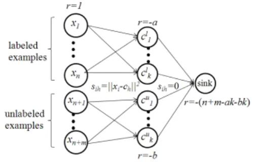
For our problem (2), the corresponding Minimum Cost Flow problem is shown in Figure 4. The supply nodes arex1. . . xn+mwithr= 1. There are two sets of
clus-ter cenclus-ter nodes. One set c`
1. . . c`k, each with demand 2
The square allows the size ratio between two clusters to be arbitrarily skewed asngrows. We do not want to fix the relative sizes of the decision setsa priori.
r = −a, is due to the labeled data size constraint. The other set cu1. . . cuk, each with demand r = −b,
is due to the unlabeled data size constraint. Finally, a sink demand node with r = −(n+m−ak−bk) catches all the remaining flow. The cost fromxi toch
is sih=kxi−chk2, and fromch to the sink is 0. It is
then clear that the Minimum Cost Flow problem (3) is equivalent to (2) with Tih =tih and c fixed.
Inter-estingly, (3) is proven to have integer solutions which correspond exactly to the desired cluster indicators.
Figure 4: The Minimum Cost Flow problem Once size-constrained spectral clustering is completed, then+mpoints will each have a cluster index in 1. . . k. We definekdecision sets{cCi}ki=1 by the Voronoi cells around these points: Cci = {x ∈ RD | x’s Euclidean nearest neighbor among the n+m points has cluster index i}. We train a separate predictor fbi for each
decision set using the labeled points in that decision set, and a user-specified supervised learner. During test time, an unseen point x∗ ∈ cCi is predicted as
b
fi(x∗). Therefore, the unlabeled data in our algorithm
is used merely to determine the decision sets.
4
EXPERIMENTS
Data Sets. We experimented with five synthetic (Fig-ure 5) and one real data sets. Data sets 1–3 are for regression, and 4–6 are for classification: (1). Dol-lar signcontains two intersecting manifolds. The “S” manifold has target y varying from 0 to 3π. The “|” manifold has target function y =x·3+ 13, where x·3 is the vertical dimension. White noise∼ N(0,0.012) is added to y. (2) Surface-sphere slices a 2D sur-face through a solid ball. The ball has target function
y =||x||, and the surface has y =x·2−5. (3)
Den-sity changecontains two overlapping rectangles. One rectangle is wide and sparse withy=x·1, the other is
narrow and five times as dense withy= 10−5x·1.
To-gether they produce three decision sets. (4) Surface-helix has a 1D toroidal helix intersecting a surface. Each manifold is a separate class. (5) Martini is a composition of five manifolds (classes) to form the shape of a martini glass with an olive on a toothpick, as shown in Figure 5(e). (6) MNISTdigits. We scaled
0 200 400 600 0 5 10 15 20 25 n MSE Global SSL Clairvoyant 0 200 400 600 0 2 4 6 8 10 n MSE Global SSL Clairvoyant 0 200 400 600 0 5 10 n MSE Global SSL Clairvoyant 0 200 400 600 0 0.1 0.2 0.3 0.4 0.5 n Error rate Global SSL 0 200 400 600 0 0.1 0.2 0.3 n Error rate Global SSL
(a) Dollar sign (b) Surface-sphere (c) Density change (d) Surface-helix (e) Martini Figure 5: Regression MSE (a-c) and classification error (d-e) for synthetic data sets. All curves are based on M = 20000, 10-trial averages, and error bars plot±1 standard deviation. Clairvoyant classification error is 0.
down the images to 16 x 16 pixels and used the official train/test split, with different numbers of labeled and unlabeled examples sampled from the training set.
Methodology & Implementation Details. In all experiments, we report results that are the average of 10 trials over random draws ofM unlabeled andn la-beled points. We compare three learners: [Global]: supervised learner trained on all of the labeled data, ignoring unlabeled data. [Clairvoyant]: with the knowledge of the true decision sets, trains one su-pervised learner per decision set. [SSL]: our semi-supervised learner that discovers the decision sets us-ing unlabeled data, then trains one supervised learner per decision set. After training, each classifier is eval-uated on a massive test set, also sampled from the un-derlying distribution, to estimate generalization error. We implemented the algorithms in MATLAB, with Minimum Cost Flow solved by the network simplex method in CPLEX. We used the same set of param-eters for all experiments and all data sets: We chose the number of decision sets to be k = d0.5 log(n)e. To obtain the subset of m unlabeled points, we let the neighborhood size |N(x)| = b3 log(M)c. When creating the graphW, we usedb1.5log(m+n)c near-est Mahalanobis neighbors, and an RBF bandwidth σ= 0.2 to convert Hellinger distances to edge weights. The size constraints were a = b1.25n/log2(n)c, b =
b1.25m/log2(n)c. Finally, to avoid poor local optima in spectral clustering, we ran 10 random restarts for constrained k-means, and chose the result with the lowest objective. For the regression tasks, we used kernel regression with an RBF kernel, and tuned the bandwidth parameter with 5-fold cross validation us-ing only labeled data in each decision set (or glob-ally for “Global”). For classification, we used a sup-port vector machine (LIBSVM) with an RBF kernel, and tuned its bandwidth and regularization parame-ter with 5-fold cross validation. We used Euclidean distance in each decision region for the supervised
learner, but we expect performance with geodesic dis-tance would be even better.
Results of Large M: Figure 5 reports the results for the five synthetic data sets. In all cases, we used M = 20000, n ∈ {20,40,80,160,320,640}, and the resulting regressors/classifiers are evaluated in terms of MSE or error rate using a test set of 20000 points. These results show that our SSL algorithm can dis-cover multiple manifolds and changes in density well enough to consistently outperform SL in both regres-sion and classification settings of varying complexity3. We also observed that even under- or over-partitioning into fewer or more decision sets than manifolds can still improve SSL performance4.
We performed three experiments with the digit recog-nition data: binary classification of the digits 2 vs 3, and three-way classification of 1,2,3 and 7,8,9. Here, we fixed n = 20, M = 5000, 10 random training tri-als, each tested on the official test set. Table 2 con-tains results averaged over these trials. SSL outper-forms Global in all three digit tasks, and all differences are statistically significant (α = 0.05). Note that we used the same parameters as the synthetic data exper-iments, which results ink= 2 decision sets forn= 20; again, the algorithm performs well even when there are fewer decision sets than classes. Close inspection re-vealed that our clustering step creates relatively pure decision sets. For the binary task, this leads to two
3Though not shown in Figure 5, we found that a
standard graph-based SSL algorithm manifold regulariza-tion (Belkin et al. 2006), using EuclideankNN graphs with RBF weights and all parameters tuned using cross valida-tion, performs worse than Global on these datasets due to the strong connections across manifolds.
4
We compared Global and SSL’s 10 trials at each n using two-tailed paired t-tests. SSL was statistically sig-nificantly better (α= 0.05) in the following cases: dollar sign atn= 20–80, density atn= 40–640, surface-helix at n= 20–320, and martini atn= 40–320. The two methods were statistically indistinguishable in other cases.
Table 2: 10-trial average test set error rates ± one standard deviation for handwritten digit recognition.
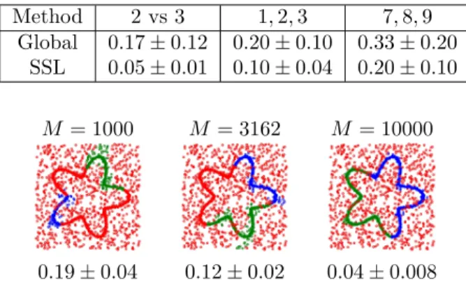
Method 2 vs 3 1,2,3 7,8,9
Global 0.17±0.12 0.20±0.10 0.33±0.20 SSL 0.05±0.01 0.10±0.04 0.20±0.10
M = 1000 M = 3162 M = 10000
0.19±0.04 0.12±0.02 0.04±0.008 Figure 6: Effect of varyingM for the surface-helix data set (n= 80). See text for details.
trivial classification problems, and errors are due only to incorrect assignments of test points to decision sets. For the 3-way tasks, the algorithm creates 1+2 and 3 clusters, and 7+9 and 8 clusters.
Effect of Too Small an M: Finally, we examine our SSL algorithm’s performance with less unlabeled data. For the surface-helix data set, we now fixn= 80 (which leads to k = 3 decision sets) and reduce M. Figure 6 depicts example partitionings for three M
values, along with 10-trial average error rates (±one standard deviation) in each setting. Note these are top-down views of the data in Figure 5(d). When M
is small, the resulting subset of m unlabeled points is too small, and the partition boundaries cannot be reliably estimated. Segments of the helix shown in red and areas of the surface in blue or green correspond to such partitioning errors. Nevertheless, even whenMis as small as 1000, SSL’s performance is no worse than Global supervised learning, which achieves an error rate of 0.20±0.05 whenn= 80 (see Figure 5(d)).
Conclusions: We have extended SSL theory and
practice to multi-manifolds. A detailed analysis of geodesic distances, automatic parameter selection, and large scale empirical study remains as future work.
Acknowledgements We thank the Wisconsin
Alumni Research Foundation. AG is supported in part by a Yahoo! Key Technical Challenges Grant.
References
Balcan, M.-F. & Blum, A. (2005), A PAC-style model for learning from labeled and unlabeled data,in‘COLT’. Basu, S., Davidson, I. & Wagstaff, K., eds (2008), Con-strained Clustering: Advances in Algorithms, Theory, and Applications, Chapman & Hall/CRC Press. Belkin, M., Sindhwani, V. & Niyogi, P. (2006), ‘Manifold
regularization: A geometric framework for learning from examples’,JMLR7, 2399–2434.
Ben-David, S., Lu, T. & Pal, D. (2008), Does unlabeled
data provably help? worst-case analysis of the sample complexity of semi-supervised learning,in‘COLT’. Bernstein, M., de Silva, V., Langford, J. & Tenenbaum, J.
(2000), Graph approximations to geodesics on embed-ded manifolds, Technical report, Stanford.
Bickel, P. & Li, B. (2007), ‘Local polynomial regression on unknown manifolds’,Complex datasets and inverse problems: Tomography, Networks and Beyond, IMS Lecture Notes-Monograph Series54, 177–186. Bradley, P., Bennett, K. & Demiriz, A. (2000), Constrained
k-means clustering, Technical Report MSR-TR-2000-65, Microsoft Research.
Chapelle, O., Zien, A. & Sch¨olkopf, B., eds (2006), Semi-supervised learning, MIT Press.
Chen, G. & Lerman, G. (2008), Spectral curvature cluster-ing,in‘IJCV’.
Demiriz, A., Bennett, K. & Embrechts, M. (1999), ‘Semi-supervised clustering using genetic algorithms’, Arti-ficial Neural Networks in Engineering.
El-Yaniv, R. & Gerzon, L. (2005), ‘Effective transductive learning via objective model selection’,Pattern Recog-nition Letters26(13), 2104–2115.
Haro, G., Randall, G. & Sapiro, G. (2008), ‘Translated poisson mixture model for stratification learning’, IJCV80, 358–374.
Joachims, T. (2003), Transductive learning via spectral graph partitioning,in‘ICML’.
Kaariainen, M. (2005), Generalization error bounds using unlabeled data,in‘COLT’.
Kushnir, D., Galun, M. & Brandt, A. (2006), ‘Fast multi-scale clustering and manifold identification’, Pattern Recognition39, 1876–1891.
Lafferty, J. & Wasserman, L. (2007), Statistical analysis of semi-supervised regression,in‘NIPS’.
Ma, Y., Derksen, H., Hong, W. & Wright, J. (2007), ‘Seg-mentation of multivariate mixed data via lossy coding and compression’,PAMI29(9), 1546–1562.
Mordohai, P. & Medioni, G. (2005), Unsupervised dimen-sionality estimation and manifold learning in high-dimensional spaces by tensor voting,in‘IJCAI’. Niyogi, P. (2008), Manifold regularization and
semi-supervised learning: Some theoretical analyses, Tech-nical Report TR-2008-01, CS Dept, U. of Chicago. Rigollet, P. (2007), ‘Generalization error bounds in
semi-supervised classification under the cluster assump-tion’,JMLR8, 1369–1392.
Singh, A., Nowak, R. & Zhu, X. (2008), Unlabeled data: Now it helps, now it doesn’t,in‘NIPS’.
Tron, R. & Vidal, R. (2007), A benchmark for the com-parison of 3-d motion segmentation algorithms, in ‘CVPR’.
Tsybakov, A. B. (2004), Introduction a l’estimation non-parametrique, Springer, Berlin Heidelberg.
Vidal, R., Ma, Y. & Sastry, S. (2008),Generalized Princi-pal Component Analysis (GPCA), Springer Verlag. von Luxburg, U. (2007), ‘A tutorial on spectral clustering’,
Statistics and Computing17(4), 395–416.
Zhou, D., Bousquet, O., Lal, T., Weston, J. & Sch¨olkopf, B. (2004), Learning with local and global consistency, in‘NIPS’.
Zhu, X. (2005), Semi-supervised learning literature survey, Technical Report 1530, Department of Computer Sci-ences, University of Wisconsin, Madison.
Zhu, X., Ghahramani, Z. & Lafferty, J. (2003), Semi-supervised learning using Gaussian fields and har-monic functions,in‘ICML’.